Virtual Rhesus Labyrinth Model Predicts Responses to Electrical Stimulation Delivered by a Vestibular Prosthesis

Abstract

To better understand the spread of prosthetic current in the inner ear and to facilitate design of electrode arrays and stimulation protocols for a vestibular implant system intended to restore sensation after loss of vestibular hair cell function, we created a model of the primate labyrinth. Because the geometry of the implanted ear is complex, accurately modeling effects of prosthetic stimuli on vestibular afferent activity required a detailed representation of labyrinthine anatomy. Model geometry was therefore generated from three-dimensional (3D) reconstructions of a normal rhesus temporal bone imaged using micro-MRI and micro-CT. For systematically varied combinations of active and return electrode location, the extracellular potential field during a biphasic current pulse was computed using finite element methods. Potential field values served as inputs to stochastic, nonlinear dynamic models for each of 2415 vestibular afferent axons, each with unique origin on the neuroepithelium and spiking dynamics based on a modified Smith and Goldberg model. We tested the model by comparing predicted and actual 3D vestibulo-ocular reflex (VOR) responses for eye rotation elicited by prosthetic stimuli. The model was individualized for each implanted animal by placing model electrodes in the standard labyrinth geometry based on CT localization of actual implanted electrodes. Eye rotation 3D axes were predicted from relative proportions of model axons excited within each of the three ampullary nerves, and predictions were compared to archival eye movement response data measured in three alert rhesus monkeys using 3D scleral coil oculography. Multiple empirically observed features emerged as properties of the model, including effects of changing active and return electrode position. The model predicts improved prosthesis performance when the reference electrode is in the labyrinth’s common crus (CC) rather than outside the temporal bone, especially if the reference electrode is inserted nearly to the junction of the CC with the vestibule. Extension of the model to human anatomy should facilitate optimal design of electrode arrays for clinical application.

INTRODUCTION

The vestibular labyrinth provides sensory input to the angular vestibulo-ocular reflex (VOR), translational VOR, ocular tilt responses, vestibulospinal, and vestibulocervical reflexes, and neural circuits that mediate perception of head orientation and movement. Failure of gaze stabilizing reflexes due to loss of labyrinthine sensation results in a dramatic drop in visual acuity during head movement (Schubert et al. 2006). This is especially problematic during high-acceleration transient head rotations, for which vision-dependent mechanisms that can otherwise partly supplant the deficient VOR fail. Loss of vestibular sensation also causes chronic disequilibrium and postural instability (Minor 1998; Grünbauer et al. 1998). Currently, vestibular rehabilitation is the only treatment with demonstrated clinical success in reducing these symptoms. The estimated worldwide prevalence of symptomatic severe bilateral vestibular loss is 1.8 M (Ward et al. 2013). Although a majority of such individuals improve with rehabilitative exercises, those who fail to do so remain disabled and suffer reduced quality of life (Sun et al. 2014).

The success of cochlear implants in restoring auditory nerve input after loss of cochlear hair cells suggests that analogous benefits might be achieved using a multichannel vestibular prosthesis (MVP) that comprises three gyros aligned with the labyrinth’s semicircular canals (SCCs) to measure three-dimensional (3D) head rotation, a processor to generate pulse-frequency-modulated biphasic pulse stimuli, and electrodes implanted near the corresponding ampullary nerves. Drawing on studies by Cohen et al. (1964) and Suzuki et al. (1969a, b) and complementing work on a single-channel head-mounted prosthesis prototype created by Gong and Merfeld (2000, 2002), Merfeld et al. (2006, 2007), and Lewis et al. (2010), we developed an MVP and demonstrated its ability to partially restore the 3D VOR in rodents and monkeys rendered insensitive to head movement via gentamicin ototoxicity (Della Santina et al. 2005, 2007; Fridman et al. 2010; Davidovics et al. 2011, 2012; Valentin et al. 2013; Dai et al. 2013).

A similar approach has been applied by others toward development of a vestibular pacing device developed in monkeys (Phillips et al. 2013, 2015; Golub et al. 2014) and intended as a treatment for Meniere’s disease in humans (Phillips et al. 2012) and a modified cochlear implant with one or more electrodes implanted in the human labyrinth (Golub et al. 2014; Pelizzone et al. 2014; Guinand et al. 2015, 2016; van de Berg et al. 2017; reviewed in Guyot and Perez Fornos 2019).

Despite promising results, misalignment between the 3D axis of the prosthetically evoked VOR response and the ideal response (i.e., the exact opposite of the head rotation, or the axis of the targeted canal when only one canal’s stimulating electrode is active) remains a challenge, because current spread and imprecision of electrode placement can result in spurious activation of vestibular afferents in nontarget nerve branches (Della Santina et al. 2007; Davidovics et al. 2011). VOR misalignment can be corrected somewhat by adjusting the 3D mapping from gyro inputs to stimulus current outputs (Fridman et al. 2010), stimulus waveform optimization can further reduce misalignment (Davidovics et al. 2011, 2013), and adaptive central nervous system circuits partly correct residual VOR misalignment (Dai et al. 2011, 2013); however, optimal design of electrode arrays and stimulus parameters is an essential first step toward achieving an effective yet selective interface with a target nerve branch by maximizing the proportion of current that activates the targeted nerve branch while minimizing current spread to nontarget nerve fibers.

Electrode position, size, and orientation; choice and location of reference electrode; use of multipolar electrode configurations; choice of stimulus waveform amplitude and shape; volume and shape of insulating carrier materials encapsulating electrode arrays; and other aspects of MVP design can all be adjusted to optimize performance. However, study of these parameters in vivo is difficult and costly in time and in the number of animals required. Systematic comparison across animals is difficult to perform because sufficiently precise and repeatable electrode positioning is difficult to accomplish with conventional surgical techniques.

Hayden et al. previously showed that a model combining realistic anatomy, finite element analysis, and a large population of axons simulated using analytic spiking neuronal models incorporating channel dynamics specific to different classes of vestibular afferent can accurately predict eye movement responses to MVP stimulation in chinchillas (Hayden 2007; Hayden et al. 2011). To facilitate design of electrodes and stimulus protocols for primates with anatomy and 3D VOR physiology closer to that of humans, we created a virtual rhesus labyrinth. In the present report, we describe the conceptual framework and technical details of the model, the assumptions underlying it, validation through comparison of model predictions to empiric data for 3D VOR responses during prosthetic stimulation over a wide range of stimulus parameters, and a series of virtual experiments performed using the model to better understand the biophysics of current flow and afferent activation in the primate labyrinth. We then use the model to investigate how prosthetically evoked 3D VOR responses should change as the reference/return electrode is repositioned from outside the temporal bone (which is typical of all currently available commercial cochlear implant stimulators) to different locations within the common crus of the implanted labyrinth (which we hypothesized should yield more selectively targeted stimulation of individual ampullary nerves).

EXPERIMENTAL METHODS

To evaluate model performance, we compared model output to archival empirical 3D VOR data previously measured during prior studies of rhesus monkeys implanted with vestibular prosthesis electrodes.

Model Overview

The virtual rhesus labyrinth model was developed by adapting a model initially created to simulate electrically evoked activity in the vestibular nerve of chinchillas (Hayden 2007; Hayden et al. 2011). We extended the approach to rhesus monkeys because of their greater similarity to humans and the existence of extensive data on their morphology, physiology, sensitivity to ototoxicity, and responses to electrical stimuli (Stein and Carpenter 1967; Carleton and Carpenter 1984; Phillips et al. 2012). A complete model description is provided in the Appendix, and the model code is available for download (http://modeldb.yale.edu/250896). In brief, a reference model geometry was defined using 3D reconstructions of micro-resolution computed tomography (CT) and magnetic resonance imaging (MRI) data sets for one normal monkey (Fig. 1). To individualize the model for a given implanted animal, the relative positions of electrodes within that animal’s labyrinth were determined using CT imaging, and spherical model electrodes were inserted in those relative locations within the ampullae of the model’s 3D geometry after coregistration of the implanted animal’s CT to the reference model geometry. Finite element analysis was performed on the resulting data sets to estimate the electrical potential field throughout the inner ear when one or more electrodes were active (Fig. 2). Extracellular potential field values were then used as input for stochastically independent, nonlinear dynamic models of action potential initiation and conduction along virtual vestibular afferents (Fig. 3), whose location and behavior were specified to reflect morphophysiologic correlations established by empiric studies (Gacek and Rasmussen 1961; Baird et al. 1988; Lysakowski and Goldberg 1997; Hayden 2007; Hayden et al. 2011). Using adaptations of extensively validated stochastic computational models for vestibular afferent spike initiation (Goldberg et al. 1984; Smith and Goldberg 1986) and action potential propagation (Frijns et al. 1994; Frijns and ten Kate 1994), the activity of a large population of model afferents was modeled. Relative proportions of afferents active in each ampullary nerve were used to predict the 3D axis of vestibulo-ocular reflex responses to electrical stimulation, after weighting to reflect the relatively weak gain of the natural VOR for head roll as compared to pitch and yaw (Migliaccio et al. 2006), and these predictions were compared to empiric data as a test of model accuracy (Figs. 1, 2, 3, and 4; Table 1).

Fig. 1.

a, b Coregistered slices through 70 μm isotropic voxel micro-CT (a) and 48 μm isotropic voxel air-contrasted T2-weighted micro-MRI (b) data sets illustrating the cristae of the anterior (a), horizontal (h), and posterior (p) semicircular canals, utricle (u), perilymphatic compartment of the vestibular near the saccule (s), and the facial nerve (f) of a normal rhesus monkey labyrinth. Air contrast in the MRI partially replaces endolymph, making borders of the saddle-shaped cristae more readily apparent against the T2-bright fluid-filled perilymphatic spaces. c, d Slices along an alternate plane transecting the anterior and horizontal canal cristae and apical half of the cochlea (c)

Fig. 2.

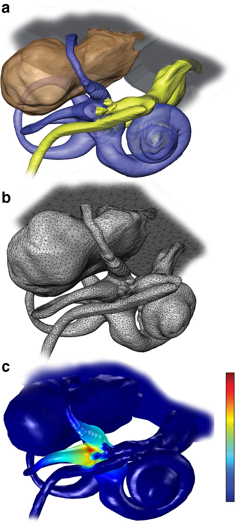
a 3D reconstructions of MRI and CT imaging data sets for a rhesus labyrinth. b Meshed model geometry for finite element analysis, including > 1 million tetrahedral elements. c Potential field and current density field estimated by finite element solution during 80 μA cathodic current delivered via a monopolar electrode in the left horizontal semicircular canal ampulla with respect to a “body” reference electrode outside the temporal bone. Color scale: electric potential normalized to unity near active electrode and zero outside the temporal bone. Note that current density scales with the electric potential gradient (i.e., rate of change in space), which is steepest in the horizontal ampulla near the stimulating electrode. Little current passes into the nearby facial nerve, because bone separates the canal lumen from the facial nerve

Fig. 3.

a One hundred model afferent starting positions in peripheral (top image), intermediate (middle), and central (bottom) zones of the posterior semicircular canal crista surface. b Representative set of fiber trajectories within the three ampullary nerve domains. c Model geometry of one model vestibular afferent (not to scale)

Fig. 4.

a Posterolateral view of 3D CT surface reconstruction showing electrode array leads implanted in the left labyrinth of a rhesus monkey via the mastoid cavity. (a) Lead to anterior and horizontal ampullae; (b) lead to posterior ampulla; (c) common crus reference electrode; (d) neck reference electrode; (M) mandibular ramus; (Z) zygomatic arch; ANT, POST, SUP, INF: anterior, posterior, superior, inferior. b Oblique CT cut through the plane of the basal turn of the cochlea (Co), showing bifurcated electrode array (a) entering the ampullae of the anterior (a-scc) and horizontal (h-scc) semicircular canals. Part of the neck reference electrode (d) is also visible, but the posterior scc electrode array is not included in this section. AM, PL: anteromedial, posterolateral. c Electrode array of the design used in all animals in this study. Implantation into the three semicircular canals (SCCs) is facilitated by consolidation of the electrodes into two silicone carriers, a forked array that positions six electrodes (e4–e9) within the anterior and horizontal ampullae and a second that positions electrodes e1–e3 in the posterior SCC ampulla. A marker dot on one side of the forked array clarifies which tine is in which ampulla; in all animals described here, e4–e6 were in the left anterior SCC ampulla and e7–e9 were in the left horizontal SCC ampulla. The microelectrode array has two reference electrodes (not shown): a large-area distant “body” reference placed outside the temporal bone (e10) and a smaller return electrode meant for insertion at the common crus of the vestibular labyrinth (e11). Although only one electrode per ampulla and one reference are required to stimulate each ampullary nerve, the presence of three electrodes per ampulla and two different references provides an opportunity to examine the effect of variation in stimulating and reference electrode locations, increases the likelihood of getting an electrode near its target nerve, allows use of bipolar and tripolar stimulation configurations, and increased the number of data sets available for testing performance of the virtual rhesus labyrinth model described in this report. a and b reproduced from Dai et al. (2013), and c reproduced from Chiang et al. (2011), with permission

Table 1.

Tissue conductivities used in the model

Tissue domain	Resistivity (Ω cm)
Vestibular lumen	50
Bone	7200
Brain	300
Nerve (longitudinal)	300
Nerve (transverse)	7000
Body	581
Air	~infinite

Animal Subjects

Three adult rhesus monkeys (5–7 kg, two females and one male) were used for all experiments, which were performed in accordance with a protocol approved by the Johns Hopkins Animal Care and Use Committee, which is accredited by the Association for the Assessment and Accreditation of Laboratory Animal Care (AAALAC) International and consistent with European Community Directive 86/609/EEC.

Experimental Design Overview

Prior to any manipulation of the labyrinths, 3D VOR responses of normal monkeys were measured in response to whole-body, passive sinusoidal and impulse rotations delivered in darkness about each of the mean SCC axes. Responses were also measured during brief steps of passive, whole-body rotational acceleration in darkness. An MVP electrode array was then implanted in the left labyrinth of each animal, and both labyrinths were treated with intratympanic gentamicin injections one or more times until VOR responses to whole-body rotation in darkness were decreased to ~ 10 % of normal. Once severe/profound reduction in VOR eye movement responses to whole-body rotation without prosthetic stimulation was confirmed, animals were adapted in light to a baseline, constant stimulation rate of 94 pulses/s (pps) on each of the three ampullary nerve stimulating electrodes until slow-phase nystagmus (an effect of asymmetry in baseline vestibular nerve activity between the implanted and nonimplanted labyrinths) reduced to < 3°/s. Animals were then typically tested for 3D VOR responses about each mean SCC axis under three experimental conditions: (1) passive whole-body rotations in darkness with only constant-rate prosthetic stimulation (mechanical-only condition); (2) pulse-frequency-modulated prosthetic electrical stimulation with the monkey stationary (prosthesis-only condition); and (3) whole-body rotation during prosthetic stimulation rate-modulated for each ampullary nerve channel by the MVP sensor detecting head motion about the corresponding axis (combined condition). To exclude influences of mechanosensation and multisensory integration, only data from the acute, head stationary, single-electrode prosthesis-only condition were used for comparison to model predictions.

Surgical Procedures

Methods used for surgical implantation of a head-fixation mechanism and scleral coils for magnetic search coil recording of 3D eye movements in primates have been described previously (Gillespie and Minor 1999; Lasker et al. 2000). With the animal under general inhalational anesthesia (2–5 % isoflurane), a light poly-ether-ether-ketone head cap was affixed to the skull under sterile conditions using titanium bone screws and poly-methyl methacrylate. Two search coils were fashioned from polytetrafluoroethylene-coated steel wire (Cooner Wire, Chatsworth, CA) and sutured to the sclera of one globe, with one around the iris and the other approximately orthogonal to the first. Wires were tightly twisted to reduce inductive artifacts and then run to connectors within the head cap. Animals were maintained under general anesthesia for surgery and treated with analgesics and antibiotics for 72 h perioperatively.

After characterization of a normal animal’s VOR responses, an electrode array was implanted into the left labyrinth via a transmastoid approach analogous to that used for cochlear implantation (Chiang et al. 2011). Under sterile conditions, a mastoidectomy was performed. The junction of the ampullae of the anterior (superior) and horizontal (lateral) SCCs was identified, and two small holes were made there, keeping a thin strut of bone intact between the two to serve as a stop when inserting the forked electrode array. An opening was also made in the thin segment of the posterior SCC near its junction with the ampulla, into which the single-tine electrode array was inserted. Pieces of fascia were tucked around each array, and a small amount of dental cement was used to stabilize the electrode leads, which were run under periosteum to the head cap.

Intratympanic gentamicin was administered using a regimen similar to that used in humans (Carey et al. 2002), except that the animal was maintained under general inhalational anesthesia (2–5 % isoflurane) for 30 min with the treated ear up to help ensure adequate diffusion of drug across the round window and into the inner ear. For each treatment, ~ 0.5 mL of 26.7 mg/mL buffered gentamicin solution injected through the ear drum into the middle ear. Delivered via this route, gentamicin accumulates in hair cells and ultimately ablates labyrinthine mechanosensitivity by destroying type I hair cells and by denuding type II hair cells of their stereocilia (Hirvonen et al. 2005; Lyford-Pike et al. 2007; Sun et al. 2015). Treatments were repeated each 3 weeks until VOR responses to head rotation toward the treated ear reduced to < 10 % of normal gain, which required two or three injections per ear in each case. About half of human patients treated with intratympanic gentamicin for Menière’s disease require more than one injection to achieve the desired drop in labyrinthine function (Nguyen et al. 2009).

Electrical Stimulation

We used a head-mounted Johns Hopkins MVP2 multichannel vestibular prosthesis (Chiang et al. 2011) with electrodes implanted in the left labyrinth of each animal. Each electrode was fashioned from Teflon®-coated 90/10 platinum/iridium wire terminating in a 250-μm-diameter hemisphere or a 200–250 μm ovoid, curved foil surface. Each electrode array comprises three subarrays, each of which in turn comprises three electrodes embedded in a silicone substrate, distributed at 600 μm center-to-center pitch along a straight line, and intended for insertion into one ampulla (Fig. 4). The subarrays intended for the anterior canal (electrodes e4, e5, and e6) and horizontal canal (electrodes e7, e8, and e9) are fused into a forked structure designed to self-orient when inserted via a pair of holes surgically drilled in those two ampullae with maintenance of a thin bone strut between them. The third array (electrodes e1, e2, and e3) is designed for insertion into the posterior canal ampulla via a surgical opening into the thin segment of the posterior canal directly medial of the posterior borders of the facial nerve’s mastoid segment and stapedius muscle. Only one stimulating electrode is required per ampulla when “monopolar” stimulation with respect to a distant reference/return electrode is used, but having multiple electrodes per ampulla increases the probability of getting at least one near the target neural tissue, allows use of bipolar and tripolar stimulation configurations, and offers an opportunity to post-operatively examine effects of a ± 600 μm variation in electrode location.

Each array also includes two reference electrodes, a “body reference” (e10) and a “common crus reference” (e11). The former is typically inserted outside the skull, beneath the temporalis muscle or in suboccipital musculature. The latter is inserted in the common crus (i.e., the common segment of the anterior and posterior canals), where it provides an alternate path for return of current from stimulating electrodes in the ampullae. This arrangement was designed in hopes of reducing aberrant stimulation of the cochlear and facial nerves that might other occur when nearly all stimulus current must leave the inner ear via the internal auditory canal en route to body reference e10.

MVP circuitry connected to the electrode array via a percutaneous connector was mounted outside the body but within the head cap to align all three gyroscopes with the corresponding mean SCC planes. The MVP delivered symmetric, biphasic, charge balanced, 200 μs/phase and 10–160 μA/phase pulse trains via each of the three ampullary electrodes with respect to a return electrode in the common crus of the left labyrinth. Each biphasic pulse comprised a constant-current cathodic phase (during which the active electrode near the target nerve was cathodic and a reference electrode was anodic), a 25 μs zero-current interphase gap, and a charge-balancing constant-current anodic phase during which the direction of current flow was reversed. Instantaneous pulse rate was defined as the reciprocal of the time from onset of one cathodic phase to the onset of the next. Pulses were presented concurrently but asynchronously, with only one electrode pair active at any given moment.

Pulse rates were modulated to encode MVP rotational velocity sensor inputs using a scheme described in detail elsewhere (Davidovics et al. 2011; Chiang et al. 2011; Dai et al. 2013). In brief, the baseline stimulation rate on each channel was 94 pulses/s, and the operating curve mapping head velocity to pulse rate was designed to emulate normal rhesus vestibular afferent rate data reported by Sadeghi et al. (2007)), consisting of a sigmoidal relationship with 47, 94, and 222 pulses/s corresponding to − 100, 0, and 100°/s, respectively, where positive values indicate head rotations excitatory for the implanted labyrinth.

To measure eye movements due solely to electrical stimulation (prosthesis-only condition), we measured VOR responses to prosthetic stimulation delivered with the head stationary and the animal seated upright in darkness. The MVP was directed to modulate pulse rates as if its sensors were encoding real sinusoidal 0.05–5 Hz, 50°/s peak rotations about each SCC axis, using the mapping functions previously defined (Lyford-Pike et al. 2007; Davidovics et al. 2011; Dai et al. 2013).

Eye Movement Measurement and Analysis

The eye coil and analysis system we used to measure 3D angular eye position and velocity has been described in detail previously (Remmel 1984; Migliaccio et al. 2004; Chiang et al. 2011; Dai et al. 2013). The monkey was seated in a plastic chair with its head restrained atraumatically by the skull cap. The chair was mounted atop the Earth-vertical-axis rotator within a gimbal that allowed us to reorient the animal to align any SCC axis with that of the rotator. Counterclockwise motor rotation as viewed from above was considered a positive sense rotation in each case, and the animal was oriented as necessary to adhere to the right-hand rule coordinate system convention used previously to describe 3D VOR data (Migliaccio et al. 2004). For example, a positive horizontal (yaw) rotation was delivered with the animal erect, and it excited the left horizontal SCC while inhibiting the right horizontal SCC. LARP axis rotations were delivered with the animal positioned supine after its head was first reoriented to turn the nose 45° toward the left ear; a positive LARP rotation excited the right posterior SCC and inhibited the left anterior SCC. RALP axis rotations were delivered with the animal positioned supine after its head was first reoriented to turn the nose 45° toward the right ear; a positive RALP rotation excited the right anterior SCC and inhibited the left posterior SCC. (A potentially confusing side effect of this standard convention is that excitation of the left labyrinth, as occurs during increases in MVP stimulation rates on that side, elicits VOR responses with horizontal, LARP, and RALP components that are negative, positive, and positive, respectively.)

Three pairs of field coils were rigidly attached to the superstructure and moved with the animal, generating three fields orthogonal to each other and aligned with the X (nasooccipital, +nasal), Y (interaural, +left), and Z (superoinferior, +superior) head coordinate axes. The X, Y, and Z fields oscillated at 79.4, 52.6, and 40.0 kHz respectively. The three frequency signals induced across each scleral coil were demodulated to produce three voltages proportional to the angles between the coil and each magnetic field, then analyzed using 3D rotational kinematic methods detailed by (Straumann et al. 2000). All signals transducing motion of the head or the eye were passed through eight-pole Butterworth anti-aliasing filters with a corner frequency of 100 Hz prior to sampling at 200 Hz. Coil misalignment was corrected using an algorithm that calculated the instantaneous rotation of the coil pair with reference to its orientation when the eye was in a reference position (Tweed et al. 1990). Angular rotations were expressed as rotation vectors with roll, pitch, and yaw coordinates, and angular velocity vectors of eye with respect to head were calculated from the corresponding rotation vectors (Hepp 1990; Haslwanter 1995; Migliaccio and Todd 1999). Angular position resolution of the coil system was 0.2° (tested over the angular range of ± 25° combined yaw, pitch, and roll positions), and angular velocity noise was ~ 2.5°/s peak.

For responses to sinusoidal stimuli, each of the three eye movement components (horizontal, LARP, and RALP) was separately averaged for > 10 cycles free of saccades and blinks. LARP and RALP axes were approximated as being 45° off the midline and in the mean plane of the horizontal SCCs. For each component of each response and for each stimulus trace, we used a single-frequency Fourier analysis to compute the magnitude of the single, symmetric best fit sinusoid to the response, under the constraint that the response frequency was the same as the known stimulus frequency.

RESULTS

Computational Performance

Finite element analysis (FEA) simulation of monopolar current injection via one intralabyrinthine electrode with respect to a distant body reference takes about 60 min on a 3.1-GHz quad core 64-bit PC running Windows 7v64. Due to the assumption of quasi-static conditions, the potential field for various multipolar electrode arrangements can be computed from a linear summation of a set of monopolar stimulation simulations, where the contribution of each electrode to the overall potential field is scaled by that electrode’s current (including polarity) for any point in time during an arbitrary stimulus current waveform. Therefore, by first performing a monopolar FEA simulation for each of the nine stimulating electrodes (taking 540 min), one can then compute the potential field for any bipolar or multipolar arrangement of those electrodes with a negligible addition of computational time.

Once the extracellular potential field has been computed using FEA, simulating spike generation and propagation for the 2415 fibers in the neuromorphic model requires about 400 min for a 2-ms duration of model time simulating responses to a single 200 μS/phase, cathodic-first (at the intralabyrinthine electrode) biphasic pulse with a 25 μS interphase gap.

Comparison of Model Predictions for 3D VOR Axis to Empirical Data

Eye movement data were acquired during stimulation delivered by each of the three stimulating electrodes in each of the three canal ampullae (electrodes e4, e5, e6 for left anterior; e7, e8, e9 for left horizontal; and e1, e2, e3 for left posterior) for each of the two reference electrodes (e10 = body/distant reference, e11=common crus reference), with cathodic-first 10–140 μA symmetric biphasic pulses (200 μS/phase, 25 μS interphase gap) sinusoidally pulse-frequency-modulated between ~ 0 and 400 pulses/S at a modulation frequency of 2 Hz. All empiric experiments for this study employed either e10 or e11 as the reference electrode. The resulting archive of data was compared against model simulations of each test condition, with which models specific to the current and the position of the stimulating electrode in the monkey being tests were used to independently “predict” the eye movement responses.

Figure 5 compares one sample set of empirically measured VOR data for monkey M067RhF with corresponding predictions from the model individualized for that animal using CT measurements of its electrode locations. Like all empiric data used for evaluation of model performance in the present study, these data were measured with the head fixed and shortly after onset of stimulation with the head stationary, prior to the start of chronic motion-modulated stimulation paradigms meant to engender vestibular compensation (which should reduce asymmetry) and directional plasticity (which can improve 3D VOR alignment over a few days; Dai et al. 2013). They should therefore be relatively free of effects due to central adaptation and directional plasticity, instead reflecting relative degrees of excitation on the different branches of the vestibular nerve in the implanted/stimulated ear.

Fig. 5.

Comparison of model predictions to empirical data for single set of 3D angular vestibulo-ocular reflex (VOR) responses to 2 Hz sinusoidally pulse-frequency-modulated, symmetric biphasic cathodic-first 200 μS/phase biphasic current pulse stimuli delivered via monopolar electrodes in the left horizontal, anterior, and posterior semicircular canals (SCC) of monkey M067RhF with its head immobile in darkness and its head-mounted vestibular prosthesis commanded to modulate its input as though the head were moving. (A–C) Anatomic axis of rotation for each SCC, which approximates the axis of the component of 3D VOR driven by activity of that canal. (D–F) Mean ± SD horizontal (red), left-anterior/right-posterior (LARP, green), and right-anterior/left-posterior (RALP, blue) components of slow-phase nystagmus measured in M067RhF during electrical stimulation via electrodes in the left horizontal (LH, (D)), left anterior (LA, (E)), and left posterior (LP, (F)) SCCs. Black sinusoid indicates equivalent head velocity waveform that would elicit the stimulus rate modulation if a vestibular prosthesis were set to its normal motion-modulated mode of action. The first half cycle of the black sinusoid signifies excitatory stimulation, which typically results in negative horizontal, positive LARP, and positive RALP eye movements when represented by the right-hand-rule coordinate reference frame used throughout this report. (G–I) Model outputs in the form of fiber recruitment curves showing the relative proportion of model axons activated in each vestibular nerve branch in the first 2 ms following a single 200 μS/phase, cathodic-first, symmetric biphasic pulse of amplitude 0.01–1 mA, as computed using models individualized to reflect the active electrode’s relative location for each case from which the empiric data in (D–F) were recorded. The vertical dashed lines indicate the current amplitudes for which the data in (D–F) were measured. (J–L) Actual measured (triangle) and model-predicted (circle) mean 3D VOR axes for the cases corresponding to those in (D–I). Vectors are normalized in amplitude to facilitate comparison of axes of rotation. Although the actual axis of measured eye rotation responses does not always align well with the axis of the ampullary nerve being targeted (likely due to current spread causing spurious stimulation of other nerve branches), the model-predicted axis fits empiric data to within ~ 20°. (M) 3D reconstruction of a computed tomography scan of F60738RhG (redrawn from Dai et al. 2013), showing best-fit planes for each SCC in the left labyrinth, along with corresponding axes defining the coordinate system used in all other panels. Note that the red axis in (A) and (J–M) is inverted to facilitate display, since excitation of the left horizontal SCC normally elicits a rightward eye rotation that would be beneath the sphere. In contrast, excitation of the LA and LP SCCs elicits right-hand-rule eye rotations about the +LARP and +RALP axes, respectively

Figure 5(D–F) shows mean ± SD slow-phase nystagmus velocity for each component of the 3D VOR measured in monkey M067RhF during steady-state responses to sinusoidally pulse-frequency-modulated trains of biphasic pulses identical to the output the prosthesis normally delivers when encoding 2 Hz, 50°/s peak sinusoidal head rotations about the left horizontal (Fig. 5(D)), left anterior (Fig. 5(E)), and left posterior (Fig. 5(F)) semicircular canal axes. In each case shown here, the stimuli were charge-balanced biphasic pulses, cathodic-first at the intra-ampulla electrode and returned via “body reference” electrode e10 outside the temporal bone. As has been reported previously for similar test conditions, slow-phase nystagmus responses align approximately with the 3D axis of the target semicircular canal and exhibit excitation-inhibition asymmetry, with larger velocities when pulse rate is highest (the first half-cycle in Fig. 5(D–F)) (Dai et al. 2013).

Figure 5(G–I) shows model predictions in the form of fiber recruitment curves showing the relative proportion of model axons activated in each vestibular nerve branch in the first 2 ms following a single 200 μS/phase, cathodic-first, symmetric biphasic pulse of amplitude 0.01–1 mA, as computed using models individualized to reflect the active electrode’s location for each case from which the empiric data in Fig. 5(D–F) were recorded. The vertical dashed lines indicate the current amplitudes for which the empiric data in Fig. 5(D–F) were measured. The fiber recruitment curves are typically sigmoidal functions of stimulus current when plotted on semilogx axes. For almost every stimulus current amplitude in these simulations, the model reports that the targeted vestibular nerve branch is activated more than other branches; however, it also predicts spurious activation of all other nerve branches, including those innervating the utricle and saccule. For stimulus currents above about 1 mA, the model predicts that nearly every vestibular nerve primary afferent neuron is excited. This is consistent with our observation that at such high currents and 200 μs/phase, VOR responses typically are strong but tend not to align well with the axis of the individual targeted semicircular canal, instead tending toward aligning with a vector sum of the three canals’ axes at very high currents.

Figure 5(J–L) shows the 3D axis of empirically measured peak slow-phase nystagmus velocities from Fig. 5(D–F) (marked by a circle, with line color in each instance matching that of the vector illustrating the anatomic axis of the targeted semicircular canal in Fig. 5(A–C)) and the corresponding model prediction (marked by a triangle). In each of these three sample cases, a model customized to accurately reflect stimulating electrode locations, return electrode location, and stimulus currents used in a specific animal performed reasonably well at predicting the empirically measured 3D VOR axis, although some misalignment between empirical and model response vectors is evident.

To assess model performance over a large number of electrode location and stimulus amplitude combinations, we performed empiric experiments, equivalent simulations, and comparisons like those in Fig. 5 for a total of 476 electrode activation experiments using each of the nine ampullary and two reference electrodes in each of the three monkeys for stimulus current amplitudes ranging from 10 to 140 μA. The data set comprised a total of 176, 184, and 116 and stimulus parameter sets in animals F234RhD, M067RhF, and F60738RhG, respectively. Table 2 details all combinations of monkey, target canal, electrode configuration, and stimulus current studied. Figure 6 compares empirical data and corresponding model predictions of 3D VOR axis for all 476 experiments, grouped by animal, reference electrode, and implanted canal. To facilitate comparison of measured and predicted 3D VOR axis over this large sample, all vectors in Fig. 6 are normalized in length. Responses ranged in velocity from ~ 0 to ~ 250°/s (Fig. 7), and vectors representing responses with peak velocity < 6° are shown using semitransparent vectors to indicate that their directions are less reliable due to a lower signal to noise ratio.

Table 2.

Electrical stimulation parameters for 476 cases tested empirically in three monkeys and modeled. For each test session, data acquired and modeled were for three electrodes in each of the three canal ampullae for each of the two reference electrodes (e10 = body/distant reference, e11 = common crus reference), with cathodic-first biphasic pulses (200 μS/phase, 25 μS interphase gap) pulse-frequency-modulated sinusoidally between ~ 0 and 400 pulses/S at a modulation frequency of 2 Hz. LA left anterior semicircular canal, LH left horizontal semicircular canal, LP left posterior semicircular canal

Animal	Target ampulla	Electrodes stimulating return		Stimulus current (μA)
F234RhD	LA	E4 E5 E6	E10 E11	10, 20, 30, 40, 50, 60, 70, 80 10, 20, 30, 40, 50, 60, 70, 80, 90,100 10, 20, 30, 40, 50, 60, 70, 80, 90,100
	LH	E7 E8 E9	E10 E11	10, 20, 30, 40, 50, 60, 70, 80, 90,100 10, 20, 30, 40, 50, 60, 70, 80, 90,100 10, 20, 30, 40, 50, 60, 70, 80, 90,100
	LP	E1 E2 E3	E10 E11	10, 20, 30, 40, 50, 60, 70, 80, 90 10, 20, 30, 40, 50, 60, 70, 80, 90 10, 20, 30, 40, 50, 60, 70, 80, 90, 100, 110,120
M067RhF	LA	E4 E5 E6	E10 E11	60, 70, 80, 90, 100, 110 60, 70, 80, 90, 100, 110 60, 70, 80, 90, 100, 110
	LH	E7 E8 E9	E10 E11	10, 20, 30, 40, 50, 60, 70, 80, 90, 100 10, 20, 30, 40, 50, 60, 70, 80, 90, 100 10, 20, 30, 40, 50, 60, 70, 80, 90, 100
	LP	E1 E2 E3	E10 E11	70, 80, 90, 100, 110, 120 70, 80, 90, 100, 110, 120, 140 70, 80, 90, 100, 110, 120
F60738RhG	LA	E4 E5 E6	E10 E11	10, 20, 30, 40, 50, 60, 70, 80, 90 10, 20, 30, 40, 50, 60, 70, 80, 90, 100 10, 20, 30, 40, 50, 60, 70, 80, 90, 100, 110, 120
	LH	E7 E8 E9	E10 E11	10, 20, 30, 40, 50, 60, 70, 80, 90, 100 10, 20, 30, 40, 50, 60, 70, 80 10, 20, 30, 40, 50, 60, 70, 80, 90
	LP	E1 E2 E3	E10 E11	4010, 20, 30, 40, 50, 60, 70, 80, 90, 100, 110 10, 20, 30, 40, 50, 60, 70, 80, 90, 100, 110, 120 10, 20, 30, 40, 50, 60, 70, 80, 90, 100, 110

Italicized entries correspond to the three specific cases depicted in Fig. 5

Fig. 6.

Comparison of model predictions to empirical 3D VOR axis data for 476 electrode activation experiments using three electrodes in each of the three left ampullae and two reference electrodes in each of three monkeys (F234RhD, M067RhF, and F60738RhG) for the stimulus current amplitudes listed in Table 2, which range from 10 to 140 μA and were either delivered with respect to a distant reference electrode e10 (a–c) or a common crus reference electrode e11 (d–f). The data set comprised a total of 176, 184, and 116 and stimulus parameter sets in animals F234RhD, M067RhF, and F60738RhG, respectively. Red, green, and blue axes show empiric VOR responses measured for stimulating in the left horizontal, left anterior, and left posterior ampullae, respectively; corresponding model simulation predictions are shown in purple, yellow, and black, respectively. Semitransparent axes represent the lowest 2.5 % of measured responses (< 6°/s), which were small enough to make measurement of axis direction noisy. To maximize visibility of all data, viewpoint with respect to the coordinate system in Fig. 5(M) is from azimuth α = + 90°, elevation φ = 0°

Fig. 7.

Histograms showing the sample distribution of peak measured excitatory VOR velocity, aggregated across all intra-ampullary electrodes, canals, and stimulus currents, and compiled separately for the e10 (body) and e11 (common crus) reference electrodes in each of the three monkeys studied. N = the total number of stimulus conditions reference electrode/monkey combination. Mean ± SD of each distribution is denoted by the horizontal lines above each histogram

Several findings are evident:

1. For both the e10 (“body”) and e11 (“common crus”) reference electrode locations, it was possible to stimulate each of the three ampullary nerves in every animal with sufficient intensity and selectivity to elicit 3D VOR responses along three linearly independent axes of rotation that approximately align with the targeted/implanted canal axes.

2. As expected, both the azimuth of the response axis differ significantly as a function of the targeted canal, as does the elevation (MANOVA: F_(2,932) > 611, p < 0.0001), but the responses for stimuli targeting the left horizontal (LH), left anterior (LA), and left posterior (LP) ampullae deviated from ideal responses perfectly aligned with the canals’ anatomic axes (Fig. 8). Specifically, the mean ± SD azimuths and elevations for VOR responses to stimuli targeting the LH, LA, and LP canals over all stimulus cases (including both references and all stimulus current levels) are (− 19.4 ± 5.1, − 32.5 ± 5.6, + 34.4 ± 6.2) and (− 63.7 ± 6.9, − 14.4 ± 2.9, − 8 ± 2.7), respectively, rather than (0, − 45, + 45) and (− 90, 0, 0).

3. Model predictions of 3D VOR axis align approximately but imperfectly with empiric data, with prediction error being greatest for cases in which the empirically measured response is small and far from the axis of the target canal. Such cases typically corresponded to low stimulus currents and empiric responses that are below the 2.5th percentile of all measured responses and therefore small compared to measurement noise. For the other 97.5 % of experiments, the mean ± SD difference in azimuth and elevation between the model’s prediction and the axis of actual VOR responses for stimuli targeting the LH, LA, and LP canals, averaged over all animals, electrodes within the given ampulla, both references and all current levels, was (− 7.1 ± 49.2, 7.5 ± 15.0, 1.7 ± 22.4) and (− 1.55 ± 13.1, − 2.5 ± 16.2, − 0.8 ± 15.0), respectively. Although the hypothesis of mean differences not being different from zero was not rejected for all cases expect differences in azimuth for stimuli targeting LA, our test lacked power to significantly demonstrate it, single sample t test results being respectively (t(149) = − 1.8, p = 0.07; t(161) = 6.15, p < 0.001; t(150) = 0.9, p = 0.34) and (t(149) = − 1.4, p = 0.13; t(161) = − 1.91, p = 0.06; t(150) = − 0.7, p = 0.45).

4. Apart from the subset of trials for which responses were small enough that the measured 3D VOR axis was noisy, the empirically measured responses are almost all within the octant of three-space that corresponds to the range of possible VOR responses one can achieve with vector sums of individual responses to excitation (without inhibition) of the implanted labyrinth’s three ampullary nerves. This is consistent with the fact that the axes depicted represent responses to the excitatory half-cycle of pulse-frequency-modulated electrical stimuli used in these experiments.

5. In comparison to body reference electrode e10, stimulation with respect to common crus reference electrode e11 resulted in a greater spatial separation of empirically measured 3D VOR response axes and slightly better alignment with the target canal’s axis for stimuli targeting the LH and LP canals, which imply a greater selectivity of stimulation. The alignment with the target canal’s axis was slightly better for stimuli targeting LA canal for stimulations with respect to electrode e10. The mean ± SD difference in azimuth and elevation between the ideal anatomical axis and the axis of actual VOR responses for stimuli targeting the LH, LA, and LP canals, averaged over all animals, electrodes within the given ampulla, and all current levels, was (− 24.4 ± 26.2, − 11.7 ± 6.9, 12.2 ± 17.4) and (− 33.9 ± 12.9, − 9.5 ± 18.7, − 10.0 ± 15.5), respectively, for body reference electrode e10 and (− 7.9 ± 35.6, − 17.5 ± 12.2, 9.7 ± 13.7) and (− 27.2 ± 11.2, − 15.5 ± 11.7, − 5.3 ± 9.3, respectively, for common crus reference electrode e11. This difference between e10 and e11 is greatest for all the three canals in animal M067RhF compared to the other animals.

Fig. 8.

Azimuth (a) and elevation (b) of the measured (red, green, and blue squares, respectively) and model-predicted (magenta, yellow, and black circles) three-dimensional vestibulo-ocular reflex (3D VOR) eye movement responses to prosthetic stimulation of the left horizontal, left anterior, and left posterior ampullae in each monkey aggregated separately for each animal and for each of the two reference electrodes across all stimulus currents and all intra-ampullary electrodes tested and modeled for this study, as summarized in Table 2 and Fig. 6

Model Predictions for Afferent Fiber Activity

Having validated the model’s ability to “predict” empiric 3D VOR axis with adequate fidelity, we examined the model’s predictions for how differences in reference electrode location may impact the absolute and relative proportions of fibers activated in each vestibular nerve branch during prosthetic stimulation. For this investigation, we focused on comparing predictions for fiber activity during stimulation with either “body” reference e10 or “common crus” reference e11.

Figure 9 shows fiber recruitment curves predicted by the model for one active electrode per canal, returning current to body reference electrode e10, for each of the three semicircular canals in each of the three monkeys. As in Fig. 5, the targeted branch of the vestibular nerve (signified by the bold curve showing the model’s prediction of fiber activation) usually has the lowest activation threshold and greatest sensitivity for the ~ 80–140 μA currents we typically found best for achieving the largest VOR response without a large misalignment of 3D VOR axis when using a body reference electrode.

Fig. 9.

a–i Model fiber recruitment curves for one active electrode per canal, returning current to body reference electrode e10, for each of the three left ampullae in each of three monkeys. In each panel, the targeted vestibular branch (signified by the bold curve) has the lowest activation threshold and greatest sensitivity for the ~ 80–140 μA currents we typically found best for achieving the largest VOR response without a large misalignment of 3D VOR axis

For horizontal canal electrodes (Fig. 10a–c), the model predicts that the anterior canal ampullary nerve is the next most activated ampullary nerve, while the converse is true for anterior canal electrodes (Fig. 10d–f). For posterior canal electrodes (Fig. 10g–i), the anterior is again the second most excited ampullary nerve, although less than when the active electrode is in the horizontal canal.

Fig. 10.

a–i Model fiber recruitment curves for one active electrode per canal, returning current to common crus electrode e11, for each of the three left ampullae in each of three monkeys. In each panel, the targeted vestibular branch (signified by the bold curve) has the lowest activation threshold and greatest sensitivity for the ~ 80–140 μA currents we typically found best for achieving the largest VOR response without a large misalignment of 3D VOR axis. Predicted fiber recruitment selectivity with respect to nontarget ampullary nerves is better than for body reference e10. Selectivity with respect to otolith endorgan activation is also better, but to a lesser degree

In every case, the utricular nerve is the second most excited nerve branch for mid-range stimulus currents, and utricular activity is especially prominent when the stimulating electrode is in the horizontal or anterior canal ampulla. This is consistent with the close anatomic proximity of the horizontal ampullary, anterior ampullary, and utricular nerve branches, which are nearly in contact with each other as they leave the labyrinth to converge about 1 mm into the internal auditory canal (IAC) to become the superior division of the vestibular nerve.

Interestingly, the model also predicts that saccular nerve activity rises rapidly as stimulus currents increase above ~ 100 μA, outpacing activation of nontarget ampullary nerves in some cases. These predicted effects on utricular and saccular afferent neurons are consistent with the fact that most stimulus current returned to a reference electrode outside the temporal bone passes through the medial wall of the vestibule into the IAC to the cerebellopontine angle and other CSF spaces, because bone and air filling the middle ear and mastoid have high resistivity (Table 1). For electrodes in the horizontal or anterior canal, relatively little spurious current reaches the posterior canal ampullary nerve, because the singular nerve canal (through which it travels) is longer, narrower, and farther from the electrode than the medial wall of the vestibule, through which utricular and saccular fibers travel via numerous perforations that combine to form a path that has lower resistance because its aggregate cross-sectional area is relatively large.

Figure 10 shows fiber recruitment curves predicted by the model for the same stimulating electrodes in Fig. 9 but with the common crus reference electrode e11 used instead of body reference e10. Comparing the two figures reveals several differences in predicted neural activity that appear to correspond to differences in the empiric data for e10 and e11 in Fig. 6:

1. For electrodes e1, e4, and e7 in monkey M067RhF’s horizontal, anterior, and posterior canals, the model correctly predicts that common crus reference e11 should yield greater stimulation selectivity and better VOR response alignment than does body reference e10. This is evident in the empiric data for Fig. 6b, e.

2. For stimulation via a posterior canal electrode, the model predicts better selectivity with e11 than with e10 for all three monkeys. This corresponds to the fact that e11 data in Fig. 6d–f are closer to the ideal direction (i.e., the RALP axis) than are the e10 data in Fig. 6a–c.

3. For stimulation via a horizontal or anterior canal electrode, the model predicts less spurious excitation of the posterior canal ampullary nerve with e11 than with e10 for all three monkeys. However, the predicted effect is only prominent for stimulus currents above the 140 μA maximum included in our empiric dataset for that animal.

Contrary to our a priori expectations that a common crus electrode would yield better selectivity than a body reference but would require higher currents to activate the target nerve branch, the model does not always predict a significant selectivity advantage for e11 over e10 for every case, and the current required to achieve 50 % activation of fibers in the target nerve is similar between e10 and e11 when averaged across all monkeys, canals, and electrodes within canals (t(54) = −0.5, p = 0.6).

Model Predictions for Effect of Changing Common Crus Reference Location

One possible explanation for variation in the relative performance of body reference e10 and common crus reference e11 from one animal to another could be variability in the location of e11 in each animal. To investigate this possibility, we systematically varied the common crus reference electrode location in a series of model simulations in which canal-stimulating electrodes were positioned near each crista in the model and the reference electrode was located at any one of the five locations along the length of the common crus, from its junction with the vestibule (designated e11.1) to the point at which the anterior and posterior canals converge (e11.5). We then generated fiber recruitment curves analogous to those in Figs. 10 and 11 for each of these common crus electrode locations and for a body reference e10.

Fig. 11.

Model fiber recruitment curves for one simulated active electrode per canal, positioned 1 mm from the center of the crista along a vector approximately normal to the crista surface in the horizontal (a–f), left anterior (g–l), or left posterior (M–R) ampullae, returning current either to one of the five simulated common crus electrodes e11.1–e11.5 positions shown in s or via a body reference e10. A small but systematic improvement in selectivity is apparent as the common crus electrode position is moved closer to the vestibule. t–v The model predicts that stimulation selectivity with respect to nontarget ampullary nerves, as quantified by the angle between the predicted VOR response axis and the anatomic axis of the target canal, is overall better for e11.1 than for any other simulated reference electrode location. s also shows the locations of the actual common crus electrodes in the monkeys tested. Notably, animal M067RhF, for which the e11 VOR responses were markedly better than e10 responses, was the only animal that had the common crus electrode inserted nearly to the vestibule in approximately the e11.1 position

Figure 11 shows the model’s fiber recruitment curves and corresponding VOR axis predictions for each case. The model predicts that a common crus reference electrode should generally outperform a “body” reference, achieving a similar level of activity on the target ampullary nerve branch for 100–200 μA stimulus currents with less stimulation of the non-target ampullary nerves, but the improved performance depends on how deeply the electrode is inserted in the common crus. For a reference near the junction of the common crus with the vestibule (position e11.1 in Fig. 11), the benefit over body reference e10 is most prominent. For positions far from the vestibule (e.g., e11.4 and e11.5 in Fig. 11), the benefit nonzero but relatively small. The model also predicts that the benefit of using a common crus reference electrode is greatest for a posterior canal-stimulating electrode, compared to the case for horizontal and anterior canal electrodes.

These model outcomes provide a context within which to understand variation between animals in our empiric VOR data. As shown in Fig. 11s, monkey M067RhF’s common crus electrode was inserted more deeply than the other monkeys’ reference electrodes. This may explain why M067RhF’s responses with common crus electrode e11 were significantly better that the e10 case whereas the other monkeys’ data and simulations did not show much difference in performance between e10 and e11. Moreover, the empiric and model data in Figs. 6, 9, and 10 show that common crus electrode e11 outperformed e10 in all monkeys for the posterior canal (albeit to a lesser degree for monkeys F234RhD and F60738RhG) compared to the other two canals, consistent with the model predictions in Fig. 11.

Comparison of Model Predictions for 3D VOR Velocity to Empirical Data

Increasing the pulse amplitude of a biphasic stimulus pulse train increases the spike probability of individual vestibular afferent neurons (Mitchell et al. 2016) and also increases the velocity of the electrically evoked VOR (Davidovics et al. 2013); however, the quantitative relationship between the proportion of vestibular afferent neurons excited by a stimulus pulse train and the resulting VOR eye movement has not yet been fully characterized. We are certain only that about that relationship’s lower and upper bounds (0 % and 100 % fiber activation above baseline spontaneous activity corresponds, respectively, to no VOR response and to the highest velocity VOR responses we ever measure with maximum possible stimuli, which can be as high as ~ 800°/s for a 100 ms, 600 pulse/s train of 225 μA/phase, 150 μs/phase biphasic pulses; Davidovics et al. 2013) and experience suggests the relationship is monotonic. Without justification for a more precise estimate, we therefore assumed that the relationship between the proportion of fibers in an ampullary nerve activated by a single pulse and the 3D VOR component of the eye movement response driven by that ampullary nerve’s activity is linear and has the same positive slope for all three ampullary nerves. (As described in “EXPERIMENTAL METHODS,” we also assumed that the slope of this relationship is zero for the utricular and saccular nerves.) By making this assumption, we could make a testable prediction about 3D VOR axis by converting the proportions of model afferent activated in each branch of the modeled vestibular nerve into a vector representing the 3D axis of head rotation the animal should “perceive” for that pattern of nerve activity, then taking the additive inverse of that vector as the estimate of 3D VOR axis, after scaling to reflect the different relative gains of roll, pitch, and yaw components of the primate VOR. Is this assumption that each component of 3D VOR velocity scales linearly with the corresponding ampullary nerve’s proportion of active afferent fibers valid?

Comparison of the model’s afferent activity predictions to measured 3D VOR velocity component data show that the assumption of linearity is a marked over-simplification. For example, Fig. 12 illustrates the relationship between each canal-axis-specific component of the empirically measured 3D VOR response velocity to the model’s predictions for the proportion of fibers active in the corresponding ampullary nerve, for every stimulating electrode in the corresponding ampulla, for reference electrodes e10 and e11, for every stimulus current presented to one monkey (F234RhD), and Fig. 13 shows analogous plots for the other monkeys. Although the relationship y = f(x) between measured VOR component velocity (y) and the proportion of model fibers activated (x) is generally a monotonically increasing function of x that can be fit acceptably using the family of cumulative Gaussian curves shown in Fig. 10, it is nonlinear and noisy, with parameters and a nonzero threshold that vary between different stimulating electrodes, different reference electrodes, different model ampullary nerves, and different eye movement components.

Fig. 12.

Component-by-component illustration of the relationship between actual/measured 3D VOR responses and model predictions for the fraction of afferents activated in each ampullary nerve, for monkey F234RhD. Each row shows data for a given implanted ampulla’s three stimulating electrodes, with data sorted by stimulating electrode, reference electrode, and VOR response component. Each column shows data for one response component (i.e., the component of the 3D VOR about the axis of a given semicircular canal). Curves are cumulative Gaussian functions fit to each data set using an iterative, nonlinear least mean square optimization. Rather than being a linear relationship with zero offset as initially assumed, the mapping from fiber activity (as simulated for each ampullary nerve by the model) and peak VOR response velocity (as measured for each canal’s component of the 3D VOR during empirical oculographic tests) is nonlinear, with sensitivity increasing as the fraction of fibers activated according to the model increases. Data are limited to those currents tested in actual experiments (Table 2)

Fig. 13.

a, b Component-by-component relationship between actual/measured 3D VOR responses and model predictions for the fraction of afferents activated in each ampullary nerve, for monkeys M067RhF and F60738RhG

Despite these departures from the naïve assumption of a linear relationship, the current iteration of the virtual rhesus labyrinth model yields model predictions of 3D VOR axis that are typically accurate to within ~ 20° (Fig. 6). To further refine the model, one could calibrate it for each individual animal by using data and naïve predictions like those shown in Figs. 6, 9, 10, 11, and 12 to fit a family of nonlinear functions f_i,j(x) for each stimulating electrode i and VOR component j, then use those animal-specific mappings in subsequent model simulations. That would allow one to perform a relatively limit, standardized set of calibration experiments and then use the model to test hypotheses about the outcomes one should observe using different stimulus waveforms and multipolar stimulation paradigms that involve simultaneous delivery of different fractions of total stimulus current via multiple electrodes in one or more ampullae. A similar iterative modeling refinement approach could help clarify the relative contributions of utricular and saccular afferent activity to the 3D VOR, if electrode arrays and stimulation paradigms can be designed to reliably limit stimulus current to those endorgans. Hageman et al. recently reported progress toward that longstanding goal, using high-density micromachined electrode arrays to selectively stimulate the utricle and saccule in chinchillas (Chow et al. 2018; Hageman et al. 2018).

Dependence on Variation in Stimulating Electrode Position

An experienced ear surgeon can reliably make movements with precision of about ~ 100 μm. (For example, stapedotomy requires perforating the stapes footplate without piercing the underlying membranous labyrinth, and the thickness of a normal human stapes footplate is ~ 50 μm (Sørensen et al. 2002).) However, despite microsurgical skill, binocular microscopy, knowledge of 3D anatomy, review of preoperative imaging, and ability to see bone landmarks intraoperatively, an otologic surgeon’s ability to ensure that stimulating electrodes end up in a predetermined intralabyrinthine location is inherently limited in accuracy and precision. Assuming a uniquely optimal intra-ampullary stimulating electrode location exists for each ampullary nerve, how accurately must a surgeon place electrodes when performing vestibular implant surgery?

To test the dependence on variation in stimulating electrode position within an ampulla, we used the model to study how fiber recruitment curves change with stimulating electrode location within an ampulla. We restricted modeling for virtual experiment to monopolar intra-ampullary electrode passing current returned to a distant body reference, with the stimulating electrodes arranged with 600 μm pitch spacing along the approximate trajectories used for electrode array insertion for all monkeys implanted in this study. Unsurprisingly, Fig. 14 shows that the electrode closest to the crista yields the greatest fiber activity recruitment at the lowest threshold in each case. This effect was greatest for the anterior canal, for which the current required to activate 50 % of that canal’s model fibers was 50 μA for e6 (the nearest electrode), 100 μA for e5, and 190 μA for e4. Evidently, positional variation on the order of 100 μm causes significant variation in fiber activation. Vestibular implant electrode array designers and aspiring implant surgeons should consider this when deciding how many electrodes to insert into the ampulla. By including two or three electrodes per ampulla and spacing them ~ 500 μm apart in a monkey (or an analogous but scaled up separation for a human labyrinth), one can help ensure that at least one electrode ends up near the optimal position, even if the stimulator used does not allow bipolar stimulation between adjacent electrodes on a given intra-ampullary electrode array (Hayden 2007; Hayden et al. 2011).

Fig. 14.

Model fiber recruitment curves for the horizontal (a), anterior (b), and posterior (c) canals of the virtual rhesus labyrinth model for each of three intra-ampullary electrodes of an electrode array like the one shown in Fig. 4c. In each case, the modeled electrode sites are centered on a line approximately along the typical trajectory used for insertion of electrode arrays in this study, and the modeled electrode sites are spaced at 600 μm center-to-center pitch. Each sphere shown in d and e represents an isopotential surface that would encompass a given electrode, which could have a nonspherical shape. The displacement of perilymph and endolymph by wires and silicone is not included in this case, but could be in a future refinement of the model anatomy. A 600-μm change in electrode location makes a large difference in the threshold current required to activate a given proportion of model neurons

DISCUSSION

A fundamental goal of inner ear implant electrode array design is to determine the electrode size, shape, material, insulating substrate, orientation, and location that maximizes each electrode’s ability to safely and effectively excite its neuronal targets (e.g., a single ampullary nerve or a specified subsection of the cochlear nerve) while minimizing surgical trauma, power consumption, and unintended stimulation of other neurons in the vestibular, cochlear, and facial nerves. The model described in this report was developed to facilitate finding solutions to that optimization problem for vestibular implant design.

It may seem obvious that one should simply place each electrode immediately adjacent to its target and as far from other neurons as possible using whatever silicone carrier is needed to hold all the wires together. However, the challenge is more difficult than might first seem apparent, as evidenced by the decades-long history of cochlear implant (CI) electrode array development. Among commercially available CIs in current use, some use electrodes that sit near the scala tympani’s lateral wall, others use precurved silicone carriers to achieve a perimodiolar location, and others are designed to put electrodes in a “midscala” position touching neither the scala tympani’s lateral wall nor the modiolus. Even after nearly a half century of refinement, the diversity and continued evolution of electrode arrays used in CIs suggest that no one design has yet proven optimal, so further iterations of design and empirical testing can be expected. The future of vestibular implant electrode array design is likely to involve a similarly iterative development path.

When empirical experimentation regarding device designs and surgical techniques is fraught with risk to human subjects (as is the case with developing a new class of implanted inner ear stimulators) and/or expensive and labor-intensive to do in animals (as is the case with vestibular implant experiments in nonhuman primates), modeling offers a means to understand the behavior of complex systems, generate quantitative and testable hypotheses, parameterize empirical data, and facilitate device design.

Extending an approach we originally developed to simulate prosthetically evoked activity in the chinchilla vestibular nerve (Hayden 2007; Hayden et al. 2011), we created an anatomically precise, customizable, and powerful model for prosthetic stimulation of the rhesus labyrinth, which approximates human anatomy more closely than do rodents. Comparing the model’s predictions to archival empirical data for tests of 54 electrode pairs in the nine semicircular canals of three unilaterally implanted monkeys, we found that the model performed well enough to justify using it as an aid for design of electrode arrays through hypothesis generation, virtual experimentation, and visualization of how current spreads in the complex geometry of the inner ear and adjacent structures. Among other insights, the model revealed a plausible explanation for our previously perplexing observation that using a reference electrode in the common crus sometimes, but not always, yields markedly better prosthesis performance than using a “body” reference electrode outside the temporal bone (as is typical of all currently marketed cochlear implants).

As with any exercise in modeling a complex system, the model described here relies on many simplifications, each of which represents an opportunity for improvement through an iterative process of virtual experimentation in the model, comparison to data from analogous empirical experiments, and implementation of model refinements that reduce the error between simulated and actual data. Key priorities for increasing the model’s accuracy, precision, and generality include (1) determining how to relate predictions for the relative number of fibers excited in each ampullary nerve to the corresponding components of 3D VOR eye velocity; (2) determining how utricular and saccular afferent fiber activity should be reflected in the model’s predictions of VOR responses; (3) accounting for displacement of conductive inner ear fluids by silicone components of electrode arrays; (4) accounting for differences in variable breadth of dendritic trees in different regions of the crista; (5) adjustment of model parameters based on single-unit vestibular afferent recordings that empirically measure data corresponding to the model’s fiber recruitment curves; (6) testing the model against empirical data for bipolar, tripolar, and other electrode configurations; (7) addition of cochlear afferents and facial nerve motoneurons in the model; (8) incorporating effects of stimulus currents acting on hair cell bodies to modulate neurotransmitter release; and (9) extension of the approach to human anatomy.

Does the Error Between Model Predictions and Measured VOR Axis Represent the Effect of Otolith-Ocular Reflexes?

As detailed in the model description in the Appendix (see Prediction of 3D VOR Eye Movement Responses from Model Afferent Activity), the current iteration of the virtual rhesus labyrinth model predicts 3D VOR axis as a weighted vector sum of the relative proportions of fibers activated in each ampullary nerve branch within the neuromorphic module of the model, ignoring otolith-ocular reflex (OOR) responses driven by activity in the utricular and saccular nerves. We neglected the effects of macular nerve activity because existing evidence suggests that eye movement responses to natural stimulation of macular nerves are modest compared to VOR responses to SCC input during natural head rotation in the spectral range of interest for a vestibular implant targeting semicircular canals (Angelaki 1998; Angelaki et al. 2000), and published studies on the OOR eye movement responses that should be elicited by selective electrical excitation of different patches on the utricular and saccular maculae have yielded conflicting results (Suzuki et al. 1969b; Fluur and Mellström 1970a, b, 1971; Curthoys 1987; Goto et al. 2003, 2004).

Should errors between model predictions and actual/empirical 3D VOR response data be interpreted as estimates of the extent to which current spread elicits electrically evoked OOR responses? Ideally, the model would so accurately estimate canal-ocular reflexes that all remaining error could be attributed to electrically evoked OOR responses. However, there are multiple potential causes for model output not to perfectly simulate empiric data. Such causes for model-vs-empiric error break into three groups: (1) error due to ignoring OOR responses; (2) errors caused by the model imperfectly simulating canal-ocular responses; and (3) all other sources of “noise” in the empirical data due to anything that is not a canal-ocular or OOR response.

Regarding the second type of error, we assume that the model imperfectly estimates canal afferent activity and imperfectly maps that activity to the canal-ocular component of VOR responses. Appendix sections Anatomic Simplifications, Biophysical Simplifications, and Physiological Simplifications describe many potential causes of this type of error. Figure 12 shows that the model’s assumption of linearity (whereby the model estimates 3D VOR axis as a vector sum of canal-specific components that scale linearly with the model’s prediction for the proportion of fibers activated in each canal’s ampullary nerve) is only an approximation to the actual nonlinear, stochastic relationships.

Regarding the third type of error, we assume that empiric eye movement data include both physiologic and nonphysiologic contributions other than purely canal-ocular and otolith-ocular responses. Those can include VOR suppression by fixation of imagined targets, gaze saccades to imagined targets, vergence-mediated changes in VOR gain and axis, effects due to eccentric starting eye position, blinks, and measurement system artifacts. We strive to minimize these non-vestibular contributions, but because available evidence from the literature suggests that eye movement responses to natural stimulation of macular nerves are small compared to canal-ocular responses during natural head rotation at the frequencies of interest for a vestibular implant intended to restore the canal-ocular VOR (Angelaki 1998; Angelaki et al. 2000), we cannot justifiably attribute model-vs-empiric error solely to OOR responses.

To examine whether 3D VOR prediction error is greatest when utricular or saccular stimulation is greatest, we used multivariate analyses of azimuth and elevation to test the hypothesis that model-vs-empirical data errors for 3D VOR axis would be greater for the deepest electrodes on each shank (e3, e7, and e6 in Fig. 14, the electrodes nearest the vestibule and presumably most likely to excite otolith-ocular responses) compared to model-vs-empiric data errors for the least deeply inserted electrode on the same shank (e1, e9, and e4) and middle electrodes (e2, e8, and e5). That analysis did not reveal a statistically significant increase in error between model and prediction for the deepest electrodes. Specifically, model vs empirical azimuth error trended insignificantly lower for the deepest electrode (MANOVA: F_(2,946) = 0.31, p = 0.7) and elevation error trended insignificantly higher for the deepest electrode (MANOVA: F_(2,946) = 0.4, p = 0.6). We then tested the hypothesis that model vs empirical azimuth and/or elevation errors are greater when the model predicts more utricle and saccule afferent activity relative to canal afferent activity. We defined a quotient Q = (#utricle fibers activated + #saccule fibers activated)/(sum of #canal fibers activated for all three canals), then compared Q to azimuth and elevation error using regression analyses. Pearson correlation coefficients relating Q to error in azimuth and error in elevation were, respectively, r = 0.006 (p = 0.8) and r = − 0.1 (p = 0.2). In summary, although it seems likely that otolith-ocular reflex responses driven by current spread to the utricle and saccule explain part of the model-vs-empiric error, the available evidence does not provide sufficient basis to conclude that model-vs-empiric error is a reliable estimate of the direction and magnitude of electrically evoked otolith-ocular reflexes.

Appendix

Model Geometry, Conductivities, and Boundary Conditions

Model geometry was generated through coregistration, segmentation, and 3D reconstruction of micro-CT and micro-MRI image stacks of a post-mortem rhesus temporal bone acquired using isotropic voxels of side lengths 70 μm without contrast and 48 μm with air contrast, respectively. Figure 1 shows representative images. We used Amira software (FEI Visualization Sciences Group, Burlington, MA) to segment and then mesh image stacks into tissue volume domains and tetrahedral elements of different conductivity including nerve, bone, brain, and inner ear fluid (Fig. 2a, b). To individualize the model for each live implanted monkey, CT scans were acquired with 0.4-mm isotropic voxels to determine actual electrode locations with respect to labyrinth landmarks. Virtual electrodes were represented in the model’s 3D geometry by 200-μm-diameter spheres at the same locations relative to landmarks in the reference anatomic data set. The 3D geometry was then meshed (divided into small, non-overlapping, tetrahedral volumes), with mesh density adaptively adjusted to be greatest where electrical potential gradients were likely to be steepest, such as immediately around an electrode.

Each of 1,142,609 tetrahedral elements was assigned a conductivity drawn from published data (Table 1) (Tasaki 1964; Geddes and Baker 1967; Kosterich et al. 1983; Suesserman and Spelman 1993; Hayden et al. 2011). Perilymph and endolymph fluid spaces were lumped into one contiguous volume-denoted vestibular lumen with a single isotropic conductivity. Neither the membranous labyrinth nor any other thin epithelial surface (e.g., osseous labyrinth endosteum, blood vessel endothelium) was explicitly included in the model, because (1) they are too thin to represent as a volume of different conductivities without compromising solvability of the finite element equations and (2) they present negligible impedance to biphasic current pulses of the 25–200 μs/phase durations typically used in a vestibular prosthesis or cochlear implant.

The 7th and 8th cranial nerves were meshed into elements that each had a long axis approximately parallel to the nerve’s axis in that region. Each element was assigned anisotropic conductivity (axial 23-fold greater than transverse) to reflect that fact that current runs along axons more readily than across them. Brainstem and cerebellum were modeled as isotropic, homogenous conductors, using the average value of conductivity between white and gray matter. Solid bone was modeled using 7200 Ω cm, an average value determined from empiric data for multiple species and a sensitivity analysis for finite element modeling in the chinchilla (Hayden 2007). A “body” domain lined the model volume’s outer edges to represent paths for flow of current from within the labyrinth to a reference electrode outside of the temporal bone. The facial nerve’s extratemporal aspect was considered to be at “body” potential. Few if any bony septae remain in the mastoid after mastoidectomy for vestibular prosthesis electrode implantation, so the middle ear and mastoid air spaces were modeled as a perfect insulator. We did not include middle ear bones (other than the stapes footplate) or spiking models of fibers in the cochlear, facial, or chorda tympani nerves in the model.

Calculation of Extracellular Potential Field

Finite element analysis (FEA) was performed using the DC Conductive Media Module in COMSOL Multiphysics (COMSOL Inc., Burlington, MA) using the conjugate gradient method. We assumed quasistatic conditions (i.e., that all tissues are purely conductive without any reactance). This is a common and well-justified assumption for models of this type (Malmivuo and Plonsey 1995; Spelman et al. 1995), because dielectric relaxation times of biological tissues are much shorter than stimulus pulses used in MVPs. For any given constellation of active electrodes passing current, the 3D potential field and current density vector field were computed for each mesh vertex for a unit stimulus current (Fig. 2c). To determine the potential at any point in the volume, one can then interpolate between mesh vertices. To determine the potential at that point in space as a function of time during a train of stimulus pulses, one can multiply the unit-current potential by the stimulus current as a function of time. Using this approach does not mean that the overall model lacks realistic temporal dynamics or stochastic behavior, because extracellular potential outputs from the FEA serve as inputs to the stochastic, dynamic neuronal models described below.

Models of Vestibular Afferent Neurons

Each of the three ampullary nerves was represented by 505 model afferent neurons, and each of the two macular nerves (i.e., the utricular and saccular nerves) comprised 450 model neurons. We randomly chose the starting location of fibers in each of three concentric zones (central, intermediate, and peripheral) on each neuroepithelial surface, using a distribution for each zone that was uniform over most of that zone but then tapered to zero near the zone’s border with an adjacent zone. Figure 3a shows 100 such starting points in each zone for a flattened map of the posterior semicircular canal’s crista surface. For each model neuron, fiber diameter was randomly chosen from a Gaussian distribution for which the mean and variance were determined by the zone of fiber origin using previously published data for rhesus monkey vestibular nerve (Gacek and Rasmussen 1961).

Modified versions of the Smith-Goldberg model for vestibular primary afferent neuron spike discharge timing (Smith and Goldberg 1986) and the spatially extended nonlinear node (SENN) axon model (Frijns et al. 1994; Frijns and ten Kate 1994; McIntyre et al. 2002; Hayden et al. 2011) were used to simulate the subthreshold and spiking dynamics of each model afferent fiber’s heminode and axon respectively. The Smith-Goldberg model allowed simulation of fibers with different degrees of spontaneous discharge regularity, examples of which are shown in Fig. 3b. Apart from model geometry, the only parameters requiring a change from the fiber model used in the chinchilla model were the mean and variance of the fiber diameter distribution. All other parameters, including channel conductances and membrane-specific capacitance, were unchanged from those defined previously in a similar model of the chinchilla vestibular nerve (Hayden et al. 2011).

The extracellular potential field produced by the FEA was sampled at many points along each fiber to obtain inputs for an individualized model of that fiber’s activity. Each afferent fiber’s trajectory through the FEA model’s nerve domain was defined by a series of piecewise-linear segments that “grew” medially through the internal auditory canal model volume under control of a semi-automatic, stochastic algorithm that maintained relative positions of neighboring fibers as nerve branches merge (Fig. 3b). All fibers were modeled as having a 2-μm nonmyelinated distal heminode spike-initiator zone at the model’s crista surface and then a series of 300 μm internodes and 1 μm nodes of Ranvier (Fig. 3c).

Prediction of 3D VOR Eye Movement Responses from Model Afferent Activity

Like humans, monkeys exhibit VOR-mediated eye movements in darkness that are partly compensatory for head rotations over ~ 0.1–10 Hz and conjugate in 3D. When considered in head coordinates, the monkey VOR is not perfectly isotropic (i.e., gains for roll and pitch head rotations are ~ 50 % and ~ 90 %, respectively, of the gain for yaw head movements (Migliaccio et al. 2004, 2010) but it does approximately obey linear vector superposition for prosthetic stimuli delivered to combinations of ampullary nerves (Cohen et al. 1964; Cremer et al. 2000; Davidovics et al. 2013). To account for gain anisotropy, we first assumed isotropic gain to estimate the 3D axis of VOR eye rotation responses for any stimulus as a three-valued vector defined in a canal-axis coordinate system by the relative fraction of model afferents excited each ampullary nerve, then we remapped the resulting axis of rotation by decomposing it into roll, pitch, and yaw components; scaling those components by 0.5, 0.9, and 1.0, respectively, and then recombining and transforming the eye velocity vector prediction back to canal-based coordinates.

We neglected the effects of macular nerve activity when predicting 3D eye movement axes from the pattern of vestibular nerve activity reported by the model, because (1) existing evidence suggests that eye movement responses to natural stimulation of macular nerves are modest compared to VOR responses to SCC input during natural head rotation in the spectral range of interest for a vestibular implant targeting semicircular canals (Angelaki 1998; Angelaki et al. 2000) and (2) lack of published data on the VOR eye movement responses that would be elicited by selective electrical excitation of different patches on the utricular and saccular maculae.

Simplifications

Like the chinchilla labyrinth model from which it was adapted (Hayden et al. 2011), the Virtual Rhesus Labyrinth includes several simplifying assumptions regarding anatomy, biophysics and physiology.

Anatomic Simplifications

We neglected the membranous labyrinth and instead treated endolymph and perilymph as a single contiguous space with uniform isotropic conductivity. This is well justified for the brief current pulses typically used in a vestibular implant, because capacitive currents readily cross the membranous labyrinth walls; however, this assumption would lead to errors if applied to DC or low-frequency current stimuli. We neglected dura and endosteum for analogous reasons.

Rather than individualize all aspects of labyrinth anatomy when modeling a given implanted animal, we relied on a standardized labyrinth geometry created from micro-CT and micro-MRI images of a single normal rhesus temporal bone, then placed virtual electrodes in the model mesh after coregistration of an implanted animal’s micro-CT with the standard model’s geometry. Although labyrinthine anatomy is highly conserved between individual animals of a given species, there is still variation in the shape of individual structures and the orientation of the labyrinth with respect to the skull landmarks upon which we base the coordinate system for oculographic measurements of eye rotation axes, so this approximation contributes some error to model predictions of fiber activity and eye movement responses.

We did not model the diversity of post-synaptic specializations such as calyces or bouton arbors, although they are consistent features in nonhuman primates and other species and likely play important roles in determining afferent responses to natural stimuli (Baird et al. 1988; Goldberg et al. 1990). We justified this simplification because including such features would render the modeling intractable without greater computing power and because electrophysiologic measurements in squirrel monkey vestibular nerve prosthetic currents predominantly act at directly at the spike initiator zone of a primary afferent (Goldberg et al. 1984). We also ignored afferent fiber somata and efferent fibers in the vestibular nerve, and we did not model the thin cribriform bone through which nerve fascicles transit between the inner ear and the internal auditory canal.

Each of the 2415 fibers in the model is simulated as though it is alone in a conductive volume that is homogeneous apart from anisotropic conductivity that varies in direction such that the least conductive direction is perpendicular to the axis of the nerve. We did not account for changes in membrane excitability that could occur due to ephaptic transmission between adjacent axons or changes in extracellular ionic environment immediately adjacent to each node of Ranvier. The model does not yet estimate or account for the effects of vestibular efferent stimulation.

In its current form, the model does not include physiologic models of cochlear or facial nerve axons. However, those nerves are segmented as separate volumes in the model geometry, and the model does provide estimates of extracellular potential throughout the temporal bone, including the cochlea, cochlear nerve, and intratemporal course of the facial nerve, so neuromorphic models of axons in those nerves could be added to allow estimation of tinnitus, facial muscle activation, or dysgeusia as side effects of electrical stimulation intended only for the vestibular nerve.

Biophysical Simplifications

When using finite element analysis to compute the extracellular potential at each point in the model volume, we assume quasistatic conditions, meaning that temporal dynamics of the extracellular potential field can be ignored. To compute the potential for a given point in the model volume as a function of time, we then need only scale the stimulus current waveform by the extracellular potential computed for a unit stimulus current pulse. This approximation is standard for finite element modeling and is well justified in our case, because dielectric relaxation times for biological tissues are much shorter than the stimulus pulses we typically use. Spelman et al. found that quasistatic assumptions hold for stimuli up to 12.5 kHz in the cochlea (Spelman et al. 1982). For the stimuli we typically use in vestibular stimulation (symmetric 200 μS/phase biphasic pulses with 25 μS interphase gap), 95 % of the spectral energy lies below 10 kHz, and the quasistatic assumption probably incurs negligible errors. However, errors due to the quasistatic assumption would be greater when this model is applied to pulses < 50 μS/phase.

In general, tissue conductivity is frequency dependent. Fortunately, conductivities have been described for several species and tissue types; however, many tissues have only been characterized for frequencies outside of our region of interest (Geddes and Baker 1967). In such cases, we used values measured at lower frequency. Nerve and bone conductivities were chosen based on the results of a parameter sensitivity analysis described by Hayden et al. (2011)).

Physiological Simplifications

The model estimates the proportion of fibers in each vestibular nerve branch that propagate an action potential to the brainstem end of the simulated fiber within the first 2 ms after the onset of a single biphasic stimulus pulse. This duration was chosen because it is short enough to model efficiently but long enough to encompass all stimulus-driven activity in the model fibers. To model the responses of some or all simulated axons for the entire duration of a long train of stimulus pulses or any other prosthetic current waveform, one could simply run the neuromorphic models for a larger number of time steps while assigning each mesh vertex’s extracellular potential over time to equal the unit-stimulus potential multiplied by the stimulus current waveform. However, the time required to complete the simulation would scale linearly with the duration of the simulated pulse train.

Although fiber spiking dynamics were varied according to starting location on each crista or macula to reflect morphophysiologic correlations described by Goldberg et al. (1990) (Baird et al. 1988; Lysakowski et al. 1995), the neuromorphic models do not otherwise reflect variation in synapse type (i.e., calyceal versus bouton), or differential effects of prosthetic current on different branches of fibers with broadly distributed dendritic trees. Effects due to spurious activation of vestibular efferent fibers were not modeled.

Hair cells in the rhesus utricle and saccule are relatively unaffected by gentamicin at doses sufficient to severely diminish canal-ocular reflexes (Sun et al. 2015); however, absent clear guidance from the literature regarding the relationship between utricular and saccular nerve excitation patterns and the 3D axis of VOR responses, we assumed that macula-mediated responses were negligible.

Even after gentamicin treatment sufficient to ablate VOR responses to head rotation, destroy type I hair cells in rhesus canal cristae, and destroy the stereocilia of canal type II hair cells, those surviving type II hair cell bodies are still present and can probably modulate neurotransmitter release in response to prosthetic currents (Sun et al. 2015). Hair cells were not included in the present model. Errors due to excluding them were probably small for suprathreshold stimuli, given that available evidence suggests that currents delivered by stimulating electrodes in perilymph mainly act at the vestibular afferent heminode (Goldberg et al. 1984).

Apart from scaling roll, pitch, and yaw components of the predicted VOR responses by 0.7, 0.9, and 1.0, respectively, to correct for the VOR gain anisotropy observed in normal rhesus monkeys and humans (Migliaccio et al. 2006), we assumed a direct mapping from relative activation levels of one labyrinth’s three ampullary nerves to the 3D VOR components about the axes of the corresponding SCCs. Prior studies suggest that this is a reasonable approximation for the acute stimulation paradigms we used to acquire data against which the model was tested (Davidovics et al. 2011, 2013), but it ignores contributions of otolith inputs and central nervous system circuits that may remap the 3D VOR response in a space-fixed rather than canal-fixed coordinate frame (Angelaki et al. 1995; Shao et al. 2009), and it does not model effects due to habituation, long-term depression (Mitchell et al. 2016, 2017), directional plasticity (Dai et al. 2013), or changes in VOR gain due to vestibular compensation.

Funding Information

This work was funded by NIH NIDCD (mainly R01DC009255 and partly by R01DC2390 and R0113536).

Compliance with Ethical Standards

Conflict of Interest

CDS is CEO of and holds an equity interest in Labyrinth Devices LLC. The terms of these arrangements are being managed by the Johns Hopkins University in accordance with its conflict of interest policies.

References

- Angelaki DE. Three-dimensional organization of otolith-ocular reflexes in rhesus monkeys. III. Responses to translation. J Neurophysiol. 1998;80:680–695. doi: 10.1152/jn.1998.80.2.680. [DOI] [PubMed] [Google Scholar]
- Angelaki DE, Hess BJ, Suzuki J. Differential processing of semicircular canal signals in the vestibulo-ocular reflex. J Neurosci. 1995;15:7201–7216. doi: 10.1523/JNEUROSCI.15-11-07201.1995. [DOI] [PMC free article] [PubMed] [Google Scholar]
- Angelaki DE, McHenry MQ, Hess BJM. Primate translational vestibuloocular reflexes. I. High-frequency dynamics and three-dimensional properties during lateral motion. J Neurophysiol. 2000;83:1637–1647. doi: 10.1152/jn.2000.83.3.1637. [DOI] [PubMed] [Google Scholar]
- Baird RA, Desmadryl G, Fernandez C, Goldberg JM. The vestibular nerve of the chinchilla. II. Relation between afferent response properties and peripheral innervation patterns in the semicircular canals. J Neurophysiol. 1988;60:182–203. doi: 10.1152/jn.1988.60.1.182. [DOI] [PubMed] [Google Scholar]
- Carey JP, Minor LB, Peng GCY, Della Santina CC, Cremer PD, Haslwanter T. Changes in the three-dimensional angular vestibulo-ocular reflex following intratympanic gentamicin for Ménière’s disease. J Assoc Res Otolaryngol. 2002;3:430–443. doi: 10.1007/s101620010053. [DOI] [PMC free article] [PubMed] [Google Scholar]
- Carleton SC, Carpenter MB. Distribution of primary vestibular fibers in the brainstem and cerebellum of the monkey. Brain Res. 1984;294:281–298. doi: 10.1016/0006-8993(84)91040-0. [DOI] [PubMed] [Google Scholar]
- Chiang B, Fridman GY, Dai C, Rahman MA, Della Santina CC. Design and performance of a multichannel vestibular prosthesis that restores semicircular canal sensation in rhesus monkey. IEEE Trans Neural Syst Rehabil Eng. 2011;19:588–598. doi: 10.1109/TNSRE.2011.2164937. [DOI] [PMC free article] [PubMed] [Google Scholar]
- Chow M, Hageman K, Roberts D, Della Santina CC (2018) Temporal dynamics of electrically-evoked eye movements elicited by a vestibular prosthesis designed to restore sensation of gravitoinertial acceleration. ARO Abstr Volume 41:
- Cohen B, Suzuki J-I, Bender MB. XVI eye movements from semicircular canal nerve stimulation in the cat. Ann Otol Rhinol Laryngol. 1964;73:153–169. doi: 10.1177/000348946407300116. [DOI] [PubMed] [Google Scholar]
- Cremer PD, Minor LB, Carey JP, Della Santina CC. Eye movements in patients with superior canal dehiscence syndrome align with the abnormal canal. Neurology. 2000;55:1833–1841. doi: 10.1212/WNL.55.12.1833. [DOI] [PubMed] [Google Scholar]
- Curthoys IS. Eye movements produced by utricular and saccular stimulation. Aviat Space Environ Med. 1987;58:A192–A197. [PubMed] [Google Scholar]
- Dai C, Fridman GY, Chiang B, Davidovics NS, Melvin TA, Cullen KE, Della Santina CC. Cross-axis adaptation improves 3D vestibulo-ocular reflex alignment during chronic stimulation via a head-mounted multichannel vestibular prosthesis. Exp Brain Res. 2011;210:595–606. doi: 10.1007/s00221-011-2591-5. [DOI] [PMC free article] [PubMed] [Google Scholar]
- Dai C, Fridman GY, Chiang B, Rahman MA, Ahn JH, Davidovics NS, Della Santina CC. Directional plasticity rapidly improves 3D vestibulo-ocular reflex alignment in monkeys using a multichannel vestibular prosthesis. J Assoc Res Otolaryngol. 2013;14:863–877. doi: 10.1007/s10162-013-0413-0. [DOI] [PMC free article] [PubMed] [Google Scholar]
- Davidovics NS, Fridman GY, Chiang B, Della Santina CC. Effects of biphasic current pulse frequency, amplitude, duration, and interphase gap on eye movement responses to prosthetic electrical stimulation of the vestibular nerve. IEEE Trans Neural Syst Rehabil Eng. 2011;19:84–94. doi: 10.1109/TNSRE.2010.2065241. [DOI] [PMC free article] [PubMed] [Google Scholar]
- Davidovics NS, Fridman GY, Della Santina CC. Co-modulation of stimulus rate and current from elevated baselines expands head motion encoding range of the vestibular prosthesis. Exp Brain Res. 2012;218:389–400. doi: 10.1007/s00221-012-3025-8. [DOI] [PubMed] [Google Scholar]
- Davidovics NS, Rahman MA, Dai C, Ahn JH, Fridman GY, Della Santina CC. Multichannel vestibular prosthesis employing modulation of pulse rate and current with alignment precompensation elicits improved VOR performance in monkeys. J Assoc Res Otolaryngol. 2013;14:233–248. doi: 10.1007/s10162-013-0370-7. [DOI] [PMC free article] [PubMed] [Google Scholar]
- Della Santina C, Migliaccio A, Patel A. Electrical stimulation to restore vestibular function development of a 3-D vestibular prosthesis. Conf Proc Annu Int Conf IEEE Eng Med Biol Soc IEEE Eng Med Biol Soc Annu Conf. 2005;7:7380–7385. doi: 10.1109/IEMBS.2005.1616217. [DOI] [PMC free article] [PubMed] [Google Scholar]
- Della Santina CC, Migliaccio AA, Patel AH. A multichannel semicircular canal neural prosthesis using electrical stimulation to restore 3-D vestibular sensation. IEEE Trans Biomed Eng. 2007;54:1016–1030. doi: 10.1109/TBME.2007.894629. [DOI] [PMC free article] [PubMed] [Google Scholar]
- Fluur E, Mellström A. Utricular stimulation and oculomotor reactions. Laryngoscope. 1970;80:1701–1712. doi: 10.1288/00005537-197011000-00005. [DOI] [PubMed] [Google Scholar]
- Fluur E, Mellström A. Saccular stimulation and oculomotor reactions. Laryngoscope. 1970;80:1713–1721. doi: 10.1288/00005537-197011000-00006. [DOI] [PubMed] [Google Scholar]
- Fluur E, Mellström A. The otolith organs and their influence on oculomotor movements. Exp Neurol. 1971;30:139–147. doi: 10.1016/0014-4886(71)90228-7. [DOI] [PubMed] [Google Scholar]
- Fridman GY, Davidovics NS, Dai C, Migliaccio AA, Della Santina CC. Vestibulo-ocular reflex responses to a multichannel vestibular prosthesis incorporating a 3D coordinate transformation for correction of misalignment. J Assoc Res Otolaryngol. 2010;11:367–381. doi: 10.1007/s10162-010-0208-5. [DOI] [PMC free article] [PubMed] [Google Scholar]
- Frijns JH, ten Kate JH. A model of myelinated nerve fibres for electrical prosthesis design. Med Biol Eng Comput. 1994;32:391–398. doi: 10.1007/BF02524690. [DOI] [PubMed] [Google Scholar]
- Frijns JHM, Mooij J, ten Kate JH. A quantitative approach to modeling mammalian myelinated nerve fibers for electrical prosthesis design. IEEE Trans Biomed Eng. 1994;41:556–566. doi: 10.1109/10.293243. [DOI] [PubMed] [Google Scholar]
- Gacek RR, Rasmussen GL. Fiber analysis of the statoacoustic nerve of guinea pig, cat, and monkey. Anat Rec. 1961;139:455–463. doi: 10.1002/ar.1091390402. [DOI] [PubMed] [Google Scholar]
- Geddes LA, Baker LE. The specific resistance of biological material—a compendium of data for the biomedical engineer and physiologist. Med Biol Eng Comput. 1967;5:271–293. doi: 10.1007/BF02474537. [DOI] [PubMed] [Google Scholar]
- Gillespie MB, Minor LB. Prognosis in bilateral vestibular hypofunction. Laryngoscope. 1999;109:35–41. doi: 10.1097/00005537-199901000-00008. [DOI] [PubMed] [Google Scholar]
- Goldberg JM, Smith CE, Fernandez C. Relation between discharge regularity and responses to externally applied galvanic currents in vestibular nerve afferents of the squirrel monkey. J Neurophysiol. 1984;51:1236–1256. doi: 10.1152/jn.1984.51.6.1236. [DOI] [PubMed] [Google Scholar]
- Goldberg JM, Desmadryl G, Baird RA, Fernandez C. The vestibular nerve of the chinchilla. V. Relation between afferent discharge properties and peripheral innervation patterns in the utricular macula. J Neurophysiol. 1990;63:791–804. doi: 10.1152/jn.1990.63.4.791. [DOI] [PubMed] [Google Scholar]
- Golub JS, Ling L, Nie K, Nowack A, Shepherd SJ, Bierer SM, Jameyson E, Kaneko CRS, Phillips JO, Rubinstein JT. Prosthetic implantation of the human vestibular system. Otol Neurotol. 2014;35:136–147. doi: 10.1097/MAO.0000000000000003. [DOI] [PMC free article] [PubMed] [Google Scholar]
- Gong W, Merfeld DM. Prototype neural semicircular canal prosthesis using patterned electrical stimulation. Ann Biomed Eng. 2000;28:572–581. doi: 10.1114/1.293. [DOI] [PubMed] [Google Scholar]
- Gong W, Merfeld DM. System design and performance of a unilateral horizontal semicircular canal prosthesis. IEEE Trans Biomed Eng. 2002;49:175–181. doi: 10.1109/10.979358. [DOI] [PubMed] [Google Scholar]
- Goto F, Meng H, Bai R, Sato H, Imagawa M, Sasaki M, Uchino Y. Eye movements evoked by the selective stimulation of the utricular nerve in cats. Auris Nasus Larynx. 2003;30:341–348. doi: 10.1016/j.anl.2003.07.003. [DOI] [PubMed] [Google Scholar]
- Goto F, Meng H, Bai R, Sato H, Imagawa M, Sasaki M, Uchino Y. Eye movements evoked by selective saccular nerve stimulation in cats. Auris Nasus Larynx. 2004;31:220–225. doi: 10.1016/j.anl.2004.03.002. [DOI] [PubMed] [Google Scholar]
- Grünbauer WM, Dieterich M, Brandt T. Bilateral vestibular failure impairs visual motion perception even with the head still. Neuroreport. 1998;9:1807–1810. doi: 10.1097/00001756-199806010-00025. [DOI] [PubMed] [Google Scholar]
- Guinand N, van de Berg R, Cavuscens S, Stokroos RJ, Ranieri M, Pelizzone M, Kingma H, Guyot JP, Perez-Fornos A. Vestibular implants: 8 years of experience with electrical stimulation of the vestibular nerve in 11 patients with bilateral vestibular loss. ORL J Otorhinolaryngol Relat Spec. 2015;77:227–240. doi: 10.1159/000433554. [DOI] [PubMed] [Google Scholar]
- Guinand N, Van de Berg R, Cavuscens S, et al (2016) Restoring visual acuity in dynamic conditions with a vestibular implant. Front Neurosci 10:. doi: 10.3389/fnins.2016.00577 [DOI] [PMC free article] [PubMed]
- Guyot J, Perez Fornos A. Milestones in the development of a vestibular implant. Curr Opin Neurol. 2019;32:145–153. doi: 10.1097/WCO.0000000000000639. [DOI] [PMC free article] [PubMed] [Google Scholar]
- Hageman K, Chow M, Roberts D, Della Santina CC (2018) Spatial selectivity of electrically-evoked eye movements elicited by a vestibular prosthesis designed to restore sensation of gravitoinertial acceleration. ARO Abstr Volume 41:
- Haslwanter T. Mathematics of three-dimensional eye rotations. Vis Res. 1995;35:1727–1739. doi: 10.1016/0042-6989(94)00257-M. [DOI] [PubMed] [Google Scholar]
- Hayden R 1983- (2007) A model to guide electrode design for a multichannel vestibular prosthesis. Master of Science Thesis. Johns Hopkins University
- Hayden R, Sawyer S, Frey E, Mori S, Migliaccio AA, Della Santina CC. Virtual labyrinth model of vestibular afferent excitation via implanted electrodes: validation and application to design of a multichannel vestibular prosthesis. Exp Brain Res. 2011;210:623–640. doi: 10.1007/s00221-011-2599-x. [DOI] [PMC free article] [PubMed] [Google Scholar]
- Hepp K. On Listing’s law. Commun Math Phys. 1990;132:285–292. doi: 10.1007/BF02278012. [DOI] [Google Scholar]
- Hirvonen TP, Minor LB, Hullar TE, Carey JP. Effects of intratympanic gentamicin on vestibular afferents and hair cells in the chinchilla. J Neurophysiol. 2005;93:643–655. doi: 10.1152/jn.00160.2004. [DOI] [PubMed] [Google Scholar]
- Kosterich JD, Foster KR, Pollack SR. Dielectric permittivity and electrical conductivity of fluid saturated bone. IEEE Trans Biomed Eng. 1983;30:81–86. doi: 10.1109/TBME.1983.325201. [DOI] [PubMed] [Google Scholar]
- Lasker DM, Hullar TE, Minor LB. Horizontal vestibuloocular reflex evoked by high-acceleration rotations in the squirrel monkey. III. Responses after labyrinthectomy. J Neurophysiol. 2000;83:2482–2496. doi: 10.1152/jn.2000.83.5.2482. [DOI] [PubMed] [Google Scholar]
- Lewis RF, Haburcakova C, Gong W, Makary C, Merfeld DM. Vestibuloocular reflex adaptation investigated with chronic motion-modulated electrical stimulation of semicircular canal afferents. J Neurophysiol. 2010;103:1066–1079. doi: 10.1152/jn.00241.2009. [DOI] [PMC free article] [PubMed] [Google Scholar]
- Lyford-Pike S, Vogelheim C, Chu E, Della Santina CC, Carey JP. Gentamicin is primarily localized in vestibular type I hair cells after intratympanic administration. J Assoc Res Otolaryngol. 2007;8:497–508. doi: 10.1007/s10162-007-0093-8. [DOI] [PMC free article] [PubMed] [Google Scholar]
- Lysakowski A, Goldberg JM. A regional ultrastructural analysis of the cellular and synaptic architecture in the chinchilla cristae ampullares. J Comp Neurol. 1997;389:419–443. doi: 10.1002/(SICI)1096-9861(19971222)389:3<419::AID-CNE5>3.0.CO;2-3. [DOI] [PMC free article] [PubMed] [Google Scholar]
- Lysakowski A, Minor LB, Fernandez C, Goldberg JM. Physiological identification of morphologically distinct afferent classes innervating the cristae ampullares of the squirrel monkey. J Neurophysiol. 1995;73:1270–1281. doi: 10.1152/jn.1995.73.3.1270. [DOI] [PubMed] [Google Scholar]
- Malmivuo J, Plonsey R (1995) Bioelectromagnetism: principles and applications of bioelectric and biomagnetic fields. Oxford University Press
- McIntyre CC, Richardson AG, Grill WM. Modeling the excitability of mammalian nerve fibers: influence of after potentials on the recovery cycle. J Neurophysiol. 2002;87:995–1006. doi: 10.1152/jn.00353.2001. [DOI] [PubMed] [Google Scholar]
- Merfeld DM, Gong W, Morrissey J, et al. Acclimation to chronic constant-rate peripheral stimulation provided by a vestibular prosthesis. IEEE Trans Biomed Eng. 2006;53:2362–2372. doi: 10.1109/TBME.2006.883645. [DOI] [PubMed] [Google Scholar]
- Merfeld DM, Haburcakova C, Gong W, Lewis RF. Chronic vestibulo-ocular reflexes evoked by a vestibular prosthesis. IEEE Trans Biomed Eng. 2007;54:1005–1015. doi: 10.1109/TBME.2007.891943. [DOI] [PubMed] [Google Scholar]
- Migliaccio AA, Todd MJ. Real-time rotation vectors. Australas Phys Eng Sci Med. 1999;22:73–80. [PubMed] [Google Scholar]
- Migliaccio AA, Schubert MC, Jiradejvong P, Lasker DM, Clendaniel RA, Minor LB. The three-dimensional vestibulo-ocular reflex evoked by high-acceleration rotations in the squirrel monkey. Exp Brain Res. 2004;159:433–446. doi: 10.1007/s00221-004-1974-2. [DOI] [PubMed] [Google Scholar]
- Migliaccio AA, Della Santina CC, Carey JP, Minor LB, Zee DS. The effect of binocular eye position and head rotation plane on the human torsional vestibuloocular reflex. Vis Res. 2006;46:2475–2486. doi: 10.1016/j.visres.2006.02.008. [DOI] [PubMed] [Google Scholar]
- Migliaccio AA, Minor LB, Della Santina CC. Adaptation of the vestibulo-ocular reflex for forward-eyed foveate vision. J Physiol. 2010;588:3855–3867. doi: 10.1113/jphysiol.2010.196287. [DOI] [PMC free article] [PubMed] [Google Scholar]
- Minor LB. Gentamicin-induced bilateral vestibular hypofunction. JAMA. 1998;279:541–544. doi: 10.1001/jama.279.7.541. [DOI] [PubMed] [Google Scholar]
- Mitchell DE, Della Santina CC, Cullen KE. Plasticity within non-cerebellar pathways rapidly shapes motor performance in vivo. Nat Commun. 2016;7:11238. doi: 10.1038/ncomms11238. [DOI] [PMC free article] [PubMed] [Google Scholar]
- Mitchell DE, Della Santina CC, Cullen KE. Plasticity within excitatory and inhibitory pathways of the vestibulo-spinal circuitry guides changes in motor performance. Sci Rep. 2017;7:853. doi: 10.1038/s41598-017-00956-5. [DOI] [PMC free article] [PubMed] [Google Scholar]
- Nguyen KD, Minor LB, Della Santina CC, Carey JP. Time course of repeated intratympanic gentamicin for Ménière’s disease. Laryngoscope. 2009;119:792–798. doi: 10.1002/lary.20055. [DOI] [PMC free article] [PubMed] [Google Scholar]
- Pelizzone M, Fornos AP, Guinand N, van de Berg R, Kos I, Stokroos R, Kingma H, Guyot JP. First functional rehabilitation via vestibular implants. Cochlear Implants Int. 2014;15:S62–S64. doi: 10.1179/1467010014Z.000000000165. [DOI] [PubMed] [Google Scholar]
- Phillips JO, Shepherd SJ, Nowack AL, et al (2012) Longitudinal performance of a vestibular prosthesis as assessed by electrically evoked compound action potential recording. In: 2012 Annual International Conference of the IEEE Engineering in Medicine and Biology Society. IEEE, pp 6128–6131 [DOI] [PubMed]
- Phillips C, DeFrancisci C, Ling L, Nie K, Nowack A, Phillips JO, Rubinstein JT. Postural responses to electrical stimulation of the vestibular end organs in human subjects. Exp Brain Res. 2013;229:181–195. doi: 10.1007/s00221-013-3604-3. [DOI] [PubMed] [Google Scholar]
- Phillips JO, Ling L, Nie K, Jameyson E, Phillips CM, Nowack AL, Golub JS, Rubinstein JT. Vestibular implantation and longitudinal electrical stimulation of the semicircular canal afferents in human subjects. J Neurophysiol. 2015;113:3866–3892. doi: 10.1152/jn.00171.2013. [DOI] [PMC free article] [PubMed] [Google Scholar]
- Remmel RS. An inexpensive eye movement monitor using the scleral search coil technique. IEEE Trans Biomed Eng. 1984;31:388–390. doi: 10.1109/TBME.1984.325352. [DOI] [PubMed] [Google Scholar]
- Sadeghi SG, Chacron MJ, Taylor MC, Cullen KE. Neural variability, detection thresholds, and information transmission in the vestibular system. J Neurosci. 2007;27:771–781. doi: 10.1523/JNEUROSCI.4690-06.2007. [DOI] [PMC free article] [PubMed] [Google Scholar]
- Schubert MC, Migliaccio AA, Della Santina CC. Dynamic visual acuity during passive head thrusts in canal planes. J Assoc Res Otolaryngol. 2006;7:329–338. doi: 10.1007/s10162-006-0047-6. [DOI] [PMC free article] [PubMed] [Google Scholar]
- Shao Z, Puche AC, Kiyokage E, Szabo G, Shipley MT. Two GABAergic intraglomerular circuits differentially regulate tonic and phasic presynaptic inhibition of olfactory nerve terminals. J Neurophysiol. 2009;101:1988–2001. doi: 10.1152/jn.91116.2008. [DOI] [PMC free article] [PubMed] [Google Scholar]
- Smith CE, Goldberg JM. A stochastic afterhyperpolarization model of repetitive activity in vestibular afferents. Biol Cybern. 1986;54:41–51. doi: 10.1007/BF00337114. [DOI] [PubMed] [Google Scholar]
- Sørensen MS, Dobrzeniecki AB, Larsen P, Frisch T, Sporring J, Darvann TA (2002) The visible ear: a digital image library of the temporal bone. ORL J Otorhinolaryngol Relat Spec 64(6):378–381 [DOI] [PubMed]
- Spelman FA, Clopton BM, Pfingst BE. Tissue impedance and current flow in the implanted ear. Implications for the cochlear prosthesis. Ann Otol Rhinol Laryngol Suppl. 1982;98:3–8. [PubMed] [Google Scholar]
- Spelman FA, Pfingst BE, Clopton BM, et al. Effects of electrical current configuration on potential fields in the electrically stimulated cochlea: field models and measurements. Ann Otol Rhinol Laryngol Suppl. 1995;166:131–136. [PubMed] [Google Scholar]
- Stein BM, Carpenter MB. Central projections of portions of the vestibular ganglia innervating specific parts of the labyrinth in the rhesus monkey. Am J Anat. 1967;120:281–317. doi: 10.1002/aja.1001200205. [DOI] [Google Scholar]
- Straumann D, Zee DS, Solomon D. Three-dimensional kinematics of ocular drift in humans with cerebellar atrophy. J Neurophysiol. 2000;83(3):1125–1140. doi: 10.1152/jn.2000.83.3.1125. [DOI] [PubMed] [Google Scholar]
- Suesserman MF, Spelman FA. Quantitative in vivo measurements of inner ear tissue resistivities: I. In vitro characterization. IEEE Trans Biomed Eng. 1993;40:1032–1047. doi: 10.1109/10.247802. [DOI] [PubMed] [Google Scholar]
- Sun DQ, Ward BK, Semenov YR, Carey JP, Della Santina CC. Bilateral vestibular deficiency. JAMA Otolaryngol Neck Surg. 2014;140:527–534. doi: 10.1001/jamaoto.2014.490. [DOI] [PMC free article] [PubMed] [Google Scholar]
- Sun DQ, Lehar M, Dai C, Swarthout L, Lauer AM, Carey JP, Mitchell DE, Cullen KE, Santina CCD. Histopathologic changes of the inner ear in rhesus monkeys after intratympanic gentamicin injection and vestibular prosthesis electrode array implantation. J Assoc Res Otolaryngol. 2015;16:373–387. doi: 10.1007/s10162-015-0515-y. [DOI] [PMC free article] [PubMed] [Google Scholar]
- Suzuki J-I, Goto K, Tokumasu K, Cohen B. LXXII implantation of electrodes near individual vestibular nerve branches in mammals. Ann Otol Rhinol Laryngol. 1969;78:815–826. doi: 10.1177/000348946907800414. [DOI] [PubMed] [Google Scholar]
- Suzuki JI, Tokumasu K, Goto K. Eye movements from single utricular nerve stimulation in the cat. Acta Otolaryngol. 1969;68:350–362. doi: 10.3109/00016486909121573. [DOI] [PubMed] [Google Scholar]
- Tasaki I. A new measurement of action currents developed by single nodes of Ranvier. J Neurophysiol. 1964;27:1199–1206. doi: 10.1152/jn.1964.27.6.1199. [DOI] [PubMed] [Google Scholar]
- Tweed D, Cadera W, Vilis T. Computing three-dimensional eye position quaternions and eye velocity from search coil signals. Vis Res. 1990;30:97–110. doi: 10.1016/0042-6989(90)90130-D. [DOI] [PubMed] [Google Scholar]
- Valentin NS, Hageman KN, Dai C, et al. Development of a multichannel vestibular prosthesis prototype by modification of a commercially available cochlear implant. IEEE Trans Neural Syst Rehabil Eng. 2013;21:830–839. doi: 10.1109/TNSRE.2013.2259261. [DOI] [PMC free article] [PubMed] [Google Scholar]
- van de Berg R, Guinand N, Ranieri M, Cavuscens S, Khoa Nguyen TA, Guyot JP, Lucieer F, Starkov D, Kingma H, van Hoof M, Perez-Fornos A (2017) The vestibular implant input interacts with residual natural function. Front Neurol 8. 10.3389/fneur.2017.00644 [DOI] [PMC free article] [PubMed]
- Ward BK, Agrawal Y, Hoffman HJ, Carey JP, Della Santina CC. Prevalence and impact of bilateral vestibular hypofunction. JAMA Otolaryngol Neck Surg. 2013;139:803–810. doi: 10.1001/jamaoto.2013.3913. [DOI] [PMC free article] [PubMed] [Google Scholar]