

Abstract
We proposed the first models based on recurrent neural networks (more specifically Long Short-Term Memory - LSTM) for classifying relations from clinical notes. We tested our models on the i2b2/VA relation classification challenge dataset. We showed that our segment LSTM model, with only word embedding feature and no manual feature engineering, achieved a micro-averaged f-measure of 0.661 for classifying medical problem-treatment relations, 0.800 for medical problem-test relations, and 0.683 for medical problem-medical problem relations. These results are comparable to those of the state-of-the-art systems on the i2b2/VA relation classification challenge. We compared the segment LSTM model with the sentence LSTM model, and demonstrated the benefits of exploring the difference between concept text and context text, and between different contextual parts in the sentence. We also evaluated the impact of word embedding on the performance of LSTM models and showed that medical domain word embedding help improve the relation classification. These results support the use of LSTM models for classifying relations between medical concepts, as they show comparable performance to previously published systems while requiring no manual feature engineering.
Keywords: Natural language processing, Medical relation classification, Recurrent neural network, Long Short-Term Memory, Machine learning
1. Introduction
In knowledge representation, identifying relations from text documents is important for creating or augmenting structured knowledge bases and in turn supporting question answering, inference reasoning and decision making. The task usually breaks down to annotating unstructured text with named entities and identifying the relations between these annotated entities. State-of-the-art named entity recognizers can now recognize concept with high accuracy [1], but relation extraction is not as straightforward. In the biomedical and clinical domain, extracting relations from scientific publications and clinical narratives has also been an important focus over the past decade with numerous challenges due to the complexity of language and domain specific knowledge involved [2].
Biomedical relation extraction is critical in understanding clinical notes, facilitating automated diagnostic reasoning and clinical decision making. In pathology reports, immunophenotypic features are often written as relations among medical concepts. For example, in “Studies performed at MGH reveal that the [lymphoid cells] are [CD10] positive, [BCL6] positive, and [BCL2] negative.”, “lymphoid cells”, “CD10”, “BCL6” and “BCL2” are medical concepts; “CD10”, “BCL6” and “BCL2” are biomarkers of the cell. If one only captures bag-of-words or bag-of-concepts features and do not account for how concepts are interrelated, one would fail to encode in such feature representation whether “lymphoid cells” are positive or negative for “CD10”, “BCL6” and “BCL2”. In this and many other similar situations, the relations between the biomedical concepts need to be understood in the context of syntactic and/or semantic cues in order to resolve possible ambiguities.
In a broad sense, one can define a relation as a tuple r(c1 ,c2, …, cn), n ≥ 2, where ci’s are biomedical concepts (e.g., cells, biomarkers etc.), and the ci’s are semantically and/or syntactically interconnected by an overarching relation r, as expressed in text. Note that such a definition requires a relation to at least involve two concepts and precludes either a single concept or an assertion of a single concept from being regarded as a relation. Specifically, if n is two, we call the relation a two-concept relation. In the previous sentence example, one may treat the sentence as encoding a relation between four medical concepts that are of interest. One may also use the term relation to specifically refer to two-concept relations, for example
positive-expression(lymphoid cells, CD10)
positive-expression(lymphoid cells, BCL6)
negative-expression(lymphoid cells, BCL2)
From the perspective of composite relations, one may be able to decompose a multi-concept relations using certain logics over a list of two-concept relations, for example
and(positive-expression(lymphoid cells, CD10),
positive-expression(lymphoid cells, BCL6),
negative-expression(lymphoid cells, BCL2))
In some cases, logics can become more complex than the Boolean logic when we need to understand what are often referred to as events, which are defined as grammatical objects that combine lexical elements, logical semantics and syntax [3]. For example, the ternary relation treated_by(patient, Harvoni, 8-week course) as expressed in “[the patient] was administered [Harvoni] for an [8-week course]” can be understood as an event, where the event trigger is “administered”, the theme is the Hepatitis C medication “Harvoni” and the target argument is “patient”. Clearly, with a variety of logics such as temporal logic one can represent increasingly flexible events and relations. Two-concept relations are building blocks of such compositions and the most frequent forms of relations; correctly classifying two-concept relations will produce fundamental insights on how to devise better natural language processing (NLP) algorithms for elucidating the interactions between biomedical concepts.
2. Background and Related Work
Some of the critical clinical information contained in clinical narratives can be represented by relations of concepts. Biomedical relations are critical in facilitating applications such as clinical decision making, clinical trial screening, pharmacovigilance [4–12]. Determining the exact relation between the two concepts requires an understanding of the context in which the two concepts are discussed.
Part of the advances in the state-of-the-art specialized clinical NLP systems for identifying medical problems have been documented in challenge workshops such as the yearly i2b2 (Informatics for Integrating Biology to the Bedside) Workshops, which have attracted international teams to address successive shared classification tasks. One such challenge focused in part on identifying the relations that may hold between medical problems and treatments, between mdedical problems and tests, as well as between pairs of medical problems [13]. Many systems applied Support Vector Machines (SVMs) to tackle the relation extraction task by combining lexical, syntactic, and semantic features. Some systems adopted a two-step approach by first determining the candidate pairs that did not relate to each other, and then classifying the specific relation type for the rest of the candidate pairs [14–16]. Some teams added annotated and/or unannotated external data to complement their machine learning system [15, 17]. Other teams complemented their machine learning systems with rules that capture simple linguistic patterns of relations [18].
All challenge participating systems involved heavy feature engineering; they explored lexical, semantic, syntactic, general domain and medical domain ontology features [13]. Many systems also harvested features from existing NLP pipelines such as cTakes [19] and MetaMap [20]. Systems that use many human engineered features often do not generalize well to new datasets [21]. In general domain NLP, a growing number of studies have successfully used recurrent neural networks (RNNs) combined with word embedding [22] on tasks including language modeling [23], text classification [24–27], question answering [25, 26, 28, 29], machine translation [25, 30–32], named entity recognition [33–36], and relation classification [37, 38]. Inspired by general domain successes, recent progress on applying RNNs to clinical datasets also aims to reducing the amount of engineered features and has achieved some success on modeling both structured and unstructured clinical data. For structured clinical data, Choi et al. [39] applied Gated Recurrent Unit networks (GRUs) for early detection of heart failure onset using time-stamped medical events (diagnosis, medications and procedures). They showed RNNs outperformed multiple statistical learning models including logistic regression, support vector machine (SVM), k-nearest neighbor (kNN), and multi-layer perceptron (MLP). Che et al. [40] applied GRUs to perform mortality and diagnosis code prediction using time series data consisting of physiologic measurements, lab-tests values, and prescriptions. Their GRU-based model showed better AUC than logistic regression, SVM, and random forests (RF). Lipton et al. [41] trained Long Short-Term Memory networks (LSTMs) to classify 128 diagnoses from 13 frequently but irregularly sampled clinical measurements from patients in pediatric ICU. Their model showed significant improvements with respect to several strong baselines, including multilayer perceptron trained on hand-engineered features. Razavian et al. [42] used LSTMs to predict onset of 133 diseases and conditions simultaneously based on 18 common lab tests measured over time. They showed that the LSTM learned representations outperformed a logistic regression baseline with hand engineered features. Pham et al. [43] used LSTMs to model the longitudinal records of diagnoses, medications and procedures and made dynamic predictions of future diagnoses, medications and procedures. They showed improved performance over competitive models including SVM and RF. For unstructured clinical data, Dernoncourt et al. [44] applied bi-directional LSTMs to de-identifying patient notes. They adopted two bi-directional LSTM layers, one at character level and the other at word level. Their character level embedding and LSTM aim to address data sparsity due to out-of-vocabulary tokens, misspellings, and different noun forms or verb endings. The two-layer bi-directional LSTMs showed improved de-identification performance from state-of-the-art Conditional Random Field (CRF) models. Jagannatha et al. [45] applied bidirectional RNNs using Long Short-Term Memory (LSTM) and Gated Recurrent Unit (GRU) to recognize named entities or concepts such as medications, diseases and their associated attributes (e.g. frequency of medications). Their bi-directional LSTMs showed significant improvement from state-of-the-art CRF models. We refer the reader to Miotto et al. [46] for a comprehensive review of other related deep learning approaches for healthcare applications. In general, there have been fewer studies on applying RNNs to unstructured data than those to structured data in the clinical domain. This is likely due to the lack of large clinical corpus available to train word or phrase embeddings. To address this issue, Jagannatha et al. [45] combined an EHR corpus of 99,700 clinical notes with English Wikipedia and PubMed Open Access articles to train word embedding. The recent release of 2 million clinical notes from MIMIC-III database [47] has at least partially alleviated the corpus issue. In fact Dernoncourt et al. [44] used the MIMIC-III corpus as the embedding training corpus for de-identification. We used MIMIC-III trained word-embedding to enable the clinical relation classification. Our models differ from general domain relation classification models [37, 38] in that we do not use syntactic/semantic resources (compared to Yan et al. [37]), and we explicitly distinguish the words within and surrounding the two concepts (compared to Zhou et al. [38]). To the best of our knowledge, this work is the first attempt on using recurrent neural networks to classify the medical relations between candidate concepts in the clinical notes.
3. Data
In this work, we used the relation classification data from the 2010 i2b2/VA challenge, which includes relations between medical problems and treatments (TrP), relations between medical problems and tests (TeP), as well as relations between medical problems and medical problems (PP). Each of the three categories has a list of possible relations that can potentially hold between the two concepts, thus the overall task is a multi-class classification problem. The TrP relations include:
Treatment administered for medical problem (TrAP). For example, “he was given Entresto to treat his high blood pressure”.
Treatment is not administered because of the medical problem (TrNAP). For example, “Relafen which is contraindicated because of ulcers”.
Treatment improves medical problem (TrIP). For example, “infection resolved with a full course of cephalexin”
Treatment causes medical problem (TrCP). For example, “the patient took amoxicillin for two days, which caused diarrhea”
A patient’s medical problem has deteriorated or worsened because of or in spite of a treatment being administered (TrWP). For example, “the tumor was growing despite the drain”
Treatment does not relate to the medical problem as stated in the text (None)
The TeP relations include:
Test has revealed some medical problem (TeRP). For example, “an echocardiogram revealed a pericardial effusion”
Test was performed to investigate a medical problem (TeCP). For example, “chest x-ray done to rule out pneumonia”
Test does not relate to the medical problem as stated in the text (None)
The PP relations include:
Two problems are related to each other (PIP). For example, “Azotemia presumed secondary to sepsis”
Medical problem does not relate to the medical problem as stated in the text (None)
The i2b2/VA challenge organizers split the entire dataset into training and test datasets. The test dataset is in fact larger than the training dataset, in order to better test the systems’ generalizability [13]. Table 1 shows the class distribution of relation instances in the training and test datasets respectively. For the i2b2/VA relation classification task, the concepts are given, so there is no need to run a Named Entity Recognizer for this task.
Table 1.
Distribution of relation classes in the training and test datasets. Both actual numbers and percentages are shown. “PP None” indicates None relation between medical problems. “Tep None” indicates None relation between tests and medical problems. “TrP None” indicates None relation between treatments and medical problems.
| Relation Type | Training | Training % | Test | Test % | Effective Training* |
|---|---|---|---|---|---|
| PIP | 1239 | 38.4% | 1986 | 61.6% | 1123 |
| PP None | 7349 | 39.64% | 11190 | 60.36% | 4453 |
| TeCP | 303 | 34.0% | 588 | 66.0% | 271 |
| TeRP | 1734 | 36.4% | 3033 | 63.6% | 1564 |
| TeP None | 1535 | 38.50% | 2452 | 61.50% | 1379 |
| TrAP | 1423 | 36.4% | 2487 | 63.6% | 1284 |
| TrCP | 296 | 40.0% | 444 | 60.0% | 270 |
| TrIP | 107 | 35.1% | 198 | 64.9% | 100 |
| TrNAP | 106 | 35.7% | 191 | 64.3% | 101 |
| TrWP | 56 | 28.1% | 143 | 71.9% | 48 |
| TrP None | 2329 | 40.05% | 3486 | 59.95% | 2081 |
Effective Training denotes the number of samples used to train each class. It is less than the number of samples in the training dataset due to random allocation of 10% training dataset as validation set for all relations, and down-sampling for PP relations. We refer the reader to Experiments and Results section for more detail.
4. Methods
The motivating question for this study is whether we can design recurrent neural networks (RNNs) with only word embedding features and no manual feature engineering to effectively classify the relations among medical concepts as stated in the clinical narratives. We also investigated how the RNN-based approaches differ from the state-of-the-art challenge participating systems with respect to each relation category. We first describe word embedding, then our recurrent neural network models, which include sentence level and segment level Long Short-Term Memory (LSTM) models for relation classification.
4.1. Word embedding
For NLP applications, recurrent neural network models are most used together with word embeddings. The word embedding is designed to capture semantic similarity of words. The embeddings are meaningful real-valued vectors of configurable dimension, and semantically similar words usually have close embedding vectors. Neural language modeling tools such as word2vec [48] can learn embedding vectors from an unlabeled large text corpus, based on the word’s context in different sentences. For word embedding, we experimented with pre-trained word vector on general domain corpus and in-house-trained word vector on clinical notes from MIMIC-III database [47] using word2vec tool. Of note, the MIMIC-III dataset contains clinical notes for over 46,000 patients with 2 million notes and a total of 100 million words.
4.2. Recurrent Neural Networks
Recurrent Neural Networks (RNN) are designed to capture sequential patterns present in data and have been applied to longitudinal data (temporal sequence)[39], image data (spatial sequence)[49], and text data[44] in medical domain. Text data is inherently sequential as well in that when reading a sentence, one’s understanding of previous words will help his/her understanding of subsequent words. This observation of sequential characteristics of text also holds for relation classification of clinical narratives, as evidenced by the fact that many i2b2/VA challenge participants benefit from exploration of local context in their relation classification system [13]. Compared to conventional artificial neural networks, RNNs introduce a recurrent structure on a neuron, as shown in Figure 1. The recurrent neuron as in Figure 1 c) can be unfolded into a chain-like structure with multiple copies of the same input-neuron-output triplet, each passing a message to its successor, as shown in Figure 1 d). The number of triplet copies in the chain-like structure dynamically depends on the sequence that the RNN handles. That is, reading a sentence of n words, the RNN can be thought of as having a chain of n triplet copies.
Figure 1.
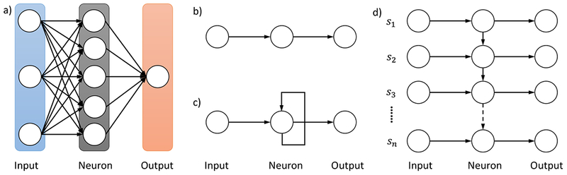
Illustration of Recurrent Neural Network structure in comparison with conventional Artificial Neural Networks. a) A conventional Artificial Neural Network. b) An input-neuron-output triplet from a conventional Artificial Neural Network. c) An input-neuron-output triplet from a Recurrent Neural Network. d) An unfolded Recurrent Neural Network upon reading a sentence of n words [s1,…,sn].
Although RNNs are capable of handling input sequences of variable sizes, they face difficulties when modeling long-term dependencies where the gap between the relevant information and the point where it is necessary becomes very large [50]. Long Short-Term Memory networks (usually abbreviated as LSTMs) are a special type of RNN that can learn long-term dependencies [51]. The recurrent neuron in RNNs, similar to the neuron on conventional Artificial Neural Networks (ANNs), has a simple activating structure, for example, h = tanh(Ws + b), where h is the output, s is the input, W is the weight matrix, and b is the bias. In LSTM networks, the recurrent neuron is equipped with a considerably more complex structure and is termed as a LSTM memory cell. More specifically, given a text sequence [s1;s2; …; sn], at each step t = 1,…,n. Let demb be the embedding size of st. Let ht and ct be the output and the state of a LSTM memory cell respectively. Let ht have a dimension of nhu, the ht’s are then pooled to produce a feature vector of dimension nhu as well. As illustrated in Figure 2 a), in step t, the LSTM cell takes as input st, ht-1, ct-1 and produces the output ht and the cell state ct based on the following formulas:
| (1) |
| (2) |
| (3) |
| (4) |
| (5) |
| (6) |
where “;” indicate vector concatenation, ft,it,ot are the values of the forget gate, input gate and output gate respectively and are each of dimension nhu, ĉt is the candidate value for the cell state and is of dimension nhu, Wf, Wi, Wc, Wo are the weight matrices and are each of dimension nhu × (demb + nhu), bf, bi, bc, bo are the bias vectors associated with corresponding gates and states and are each of dimension nhu. For operators, σ(·) and tanh (·) refer to the element-wise sigmoid and hyperbolic tangent functions, and * is the element-wise multiplication. Intuitively, ĉt corresponds to the new information one is going to store in the cell state. To derive the new cell state ct that is of dimension nhu, the forget gate ft controls what information from the old state ct-1 one wants to forget, the input gate it controls what information in ĉt one wants to use as an update. When deciding the cell output ht, the output gate ot determines which information from the cell state ct one wants to output, as in equation ( 6 ). Note that the output and the cell state from a previous step are used as input for a subsequent step, giving the recurrent nature of an LSTM memory cell.
Figure 2.
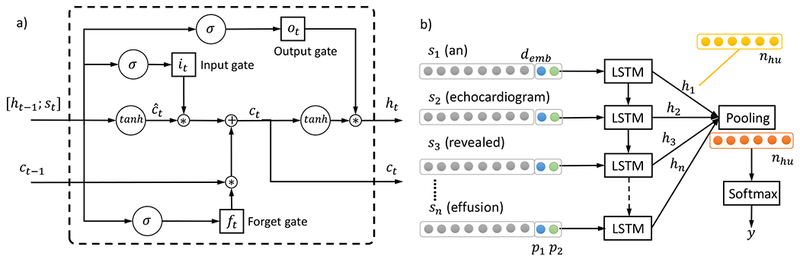
Illustration of LSTM model. a) The building blocks – LSTM memory cell. The operator “;” denotes vector concatenation, σ(·) and tanh(·) refer to the element-wise sigmoid and hyperbolic tangent functions, and * is the element-wise multiplication. The ft, it, ot are the values of the forget gate, input gate and output gate respectively, ĉt is the candidate value for the cell state, Wf, Wi, Wc, Wo are weight matrices and bf, bi, bc, bo are bias vectors associated with them. b) The sentence level LSTM model architecture for relation classification. Each LSTM block corresponds to the memory cell structure in a). Each input st, t = 1,…,n has a dimension of demb that is the word embedding size, plus two numbers p1, p2 corresponding to the distances of the current word to concept 1 and concept 2 respectively. Each LSTM memory cell output ht has a dimension of nhu, which are then pooled to produce a feature vector of dimension nhu as well. The pooling output can be regarded as the hidden units, which are input to the softmax layer that produces the label y for relation classification.
4.3. Sentence level LSTM for relation classification
The recurrent nature of a LSTM memory cell enables it to unfold when reading a sequence input. We thus propose to use the LSTM architecture as shown in Figure 2 b) to model relation classification. In order to respect the relative positions of individual words to the two medical concepts in consideration, we append to the word embedding vector two numbers p1, p2 corresponding to the distances from the current word to concept 1 and concept 2 respectively. For example in Figure 2 b), “an” is at -1 distance and “revealed” is at +1 distance away from the first concept “echocardiogram”, hence their p1 values are -1 and +1 respectively. For all words in the first concept (“echocardiogram” in this case), p1 values are set to 0. The input to LSTM memory cells is represented as a sequence of [embedding; position] vectors. We then pool the output from LSTM cells into a nhu-dimensional feature vector h, transform the feature vector into z = Whh + bh, where Wh ∈ RK×nhu, for a classification problem with K classes. We use a softmax classifier which minimizes the objective function of the K-dimensional vector z in equation ( 7 ) to obtain the class label for the concept pair.
| (7) |
For RNNs such as LSTMs, overfitting may be a serious problem. To address such a problem on sentence LSTM and other LSTM models developed in this study, we used the dropout technique [49] to randomly drop the values of a portion (50% in our experiment) of hidden units in the output of the pooling layer during training. Dropout prevents co-adaptation of these hidden units by sampling from an exponential number of different “thinned” networks, thus reduces overfitting and leads to significant improvements over other regularization methods [52].
4.4. Segment level LSTM for relation classification
The formulation of sentence level LSTM for relation classification does not explicitly distinguish the features associated with the two concepts from the features associated with the context of the two concepts. Some of the top performers in the i2b2/VA relation classification challenge reported improved performance by distinguishing the concepts vs. context text, and further differentiating the context text into text preceding the first concept, between the concepts, and succeeding the second concept [53]. To explicitly model the concept and context text, we propose the segment level LSTM architecture for relation classification, as shown in Figure 3. We divide the concept and context text into five segments: before the first concept (preceding), of the first concept (concept 1), between the two concepts (middle), of the second concept (concept 2), and after the second concept (succeeding). For each segment, we feed the sequence into a LSTM layer then a pooling layer to learn the nhu-dimensional hidden feature vector. We then concatenate the hidden features from the five segments into one 5nhu-dimensional feature vector, input the feature vector to a softmax layer to produce the relation class label. The specific sizes for each of the segment (preceding, concept 1, middle, concept 2, succeeding) in terms of the maximum number of words for a segment in the corpus are (154, 12, 153, 18, 121) for TrP relations respectively, (67, 11, 78, 31, 76) for TeP relations respectively and (125, 31, 99, 31, 78) for PP relations respectively. There is no minimum word requirement per segment, i.e., a segment can be empty in which case all-zero embedding vectors will be used to fill the necessary spaces. In the challenge dataset, some of the concepts are annotated on the head word, while others are annotated including the preceding and succeeding modifiers. There are also cases where concept annotations are on adjectives only, e.g., “temp noted to be [low]problem at 94 and she was placed on [bear hugger]treatment which improved temp to 96.7”. The issue of possible inconsistent annotation of concept boundaries seems sometimes hard to avoid and is not specific to LSTMs. In fact, many challenge participating systems used phrase chunkers (e.g., from cTakes [19], MetaMap [20], and GeniaTagger [54]) to recognize modifiers of head words in phrases [13] to address the inconsistent annotation issue. For example, the top system by Roberts et al. [53] specifically used any word used to describe the first (second) concept as features, which mitigated the effect of the inconsistent annotation of concept boundaries. To more consistently capture concept characteristics, we allow the text of the first concept to be padded before and after by neighboring words from preceding text and middle text respectively. We also padded the text of the second concept analogously. For example, in the TrIP instance “temp noted to be [low]problem at 94 and she was placed on [bear hugger]treatment which improved temp to 96.7”, with a padding size of 4, the problem concept will be padded as “temp noted to be low at 94 and she”, and the treatment concept will be padded as “she was placed on bear hugger which improved temp to”.
Figure 3.
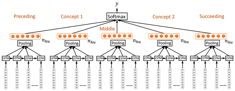
Segment level LSTM for relation classification. Concept and context text are divided into five segments: before the first concept (preceding), of the first concept (concept 1), between the two concepts (middle), of the second concept (concept 2), and after the second concept (succeeding). For each segment, the LSTM + pooling layer produced a nhu-dimensional feature vector. These vectors are then concatenated and fed into a softmax layer.
5. Experiments and Results
Our LSTM models used only word embedding features, and were compared with the i2b2/VA challenge participating systems. The types of concept 1 and concept 2 were not used as features in training and testing the LSTM models, and were only used in constructing TrP, TeP, and PP datasets. For example, if a concept pair consists of one treatment concept and one medical problem concept, they are included in the TrP dataset but not the TeP and the PP datasets. In order to make fair comparisons between our models and those from the i2b2/VA challenge participants, we adopted the same training-testing split by the challenge organizers. To optimize the hyper-parameters for our models, we further randomly selected 10% of the training dataset as the validation set. For word embedding, we experimented with the pre-trained word vectors on the Google news corpus [48] and the in-house-trained word vectors on the MIMIC-III clinical notes; both embeddings’ dimensions are 300. When inspecting relation categories, we found that the PP relations have highly imbalanced class ratio (nearly eight times more negative None relations than PIP relations). Following de Bruijn et al. [15], we down sampled the training set to a PIP/None ratio of 1:4. For segment level LSTM models, we experimented with a series of padding sizes (from 3 to 10) for padding the concept text with their context. In both sentence level and segment level LSTM models, we experimented with multiple numbers of hidden units (100, 150, and 200 in this work). Note that the number of hidden units nhu is same as the dimension of the LSTM memory cells (see Section 4.2 for more detail), not the number of LSTM memory cells. The optimal padding size, number of hidden units were chosen based on validation set performance. We used the Adadelta technique [55] – a variant of stochastic gradient descent algorithm – to optimize our loss function.
To evaluate the performance of our LSTM models, and compare them with those of the challenge participants, we computed the micro-averaged precision, recall, and F-measure. Let the set of class labels be (e.g., set of 6 labels for TrP relations), for a class k that is not “None”, let TPk be the number of true positives, FPk the number of false positives, and FNk the number of false negatives. We can calculate the micro-averaged number of true positives, false positives, and false negatives as in equation ( 8 ).
| (8) |
In turn, we can compute the micro-averaged precision Pmi, recall Rmi, and f-measure Fmi as shown in equation ( 9 ).
| (9) |
As shown in the above formulas, micro-averaging gives equal weight to each per-relation classification decision. Intuitively, Pmi is the proportion of predicted relation labels that are ground-truth labels, Rmi is the proportion of ground-truth relation labels that are correctly predicted, and Fmi is the harmonic mean of Pmi and Rmi.
We first compare our systems’ performance with those from the i2b2/VA challenge participants, as shown in Table 2. Unless otherwise mentioned, all performances are evaluated on the held-out test set. Both LSTM models in Table 2 use mean pooling. From the comparison of the micro-averaged f-measure, we see that segment LSTM model ranks the second in classifying the TrP relations, the third in TeP relation classification, and the third in PP relation classification. Although the sentence LSTM model is outperformed by the segment LSTM model in TrP and TeP relations, it does attain the best performance for PP relations. Overall segment LSTM achieves good performance that are comparable to state-of-the-art systems from i2b2/VA challenge participants with heavily engineered features, even though segment LSTM uses only the basic word embedding as features. In addition, the segment LSTM outperforms the sentence LSTM in more relation categories, which is consistent with our intuition on the benefits of exploring the distinction between concept text and context text, and between different contextual parts in the sentence regarding their different relative positions to the concepts. The exception with the problem-problem relation may be because both concepts are medical problems that tend to have similar context and concept text, making their distinction rather subtle and less informative regarding problem-problem relation classification.
Table 2.
Performance of the LSTM models with mean pooling word embedding trained on medical corpus. Performance of i2b2/VA challenge participating systems are also included for comparison. The segment LSTM mean (pooling) best performance was attained with 150 hidden units and pad size 6 for TrP relations, with 200 hidden units and pad size 4 for TeP relations, with 100 hidden units and pad size 4 for PP relations. The sentence LSTM mean best performance was attained with 200 hidden units for all relation categories. Best micro-averaged f-measures are in bold.
| System | Problem-Treatment (TrP) Relations | Problem-Test (TeP) Relations | Problem-Problem (PP) Relations | ||||||
|---|---|---|---|---|---|---|---|---|---|
| R | P | F | R | P | F | R | P | F | |
| Segment LSTM mean | 0.641 | 0.683 | 0.661 | 0.766 | 0.838 | 0.800 | 0.731 | 0.640 | 0.683 |
| Sentence LSTM mean | 0.623 | 0.658 | 0.640 | 0.758 | 0.794 | 0.775 | 0.728 | 0.681 | 0.704 |
| Roberts et al. [53] | 0.686 | 0.672 | 0.679 | 0.833 | 0.798 | 0.815 | 0.726 | 0.664 | 0.694 |
| deBruijn et al. [15] | 0.583 | 0.750 | 0.656 | 0.789 | 0.843 | 0.815 | 0.712 | 0.691 | 0.701 |
| Grouin et al. [18] | 0.646 | 0.647 | 0.647 | 0.801 | 0.792 | 0.797 | 0.645 | 0.670 | 0.657 |
| Patrick et al. [56] | 0.599 | 0.671 | 0.633 | 0.774 | 0.813 | 0.793 | 0.627 | 0.677 | 0.651 |
| Jonnalagadda et al. [14] | 0.679 | 0.581 | 0.626 | 0.828 | 0.765 | 0.795 | 0.730 | 0.586 | 0.650 |
| Divita et al. [17] | 0.582 | 0.704 | 0.637 | 0.782 | 0.794 | 0.788 | 0.534 | 0.710 | 0.610 |
| Solt et al. [57] | 0.629 | 0.621 | 0.625 | 0.779 | 0.801 | 0.790 | 0.711 | 0.469 | 0.565 |
| Demner-Fushman et al. [58] | 0.612 | 0.642 | 0.626 | 0.677 | 0.835 | 0.748 | 0.533 | 0.662 | 0.591 |
| Anick et al. [16] | 0.619 | 0.596 | 0.608 | 0.787 | 0.744 | 0.765 | 0.502 | 0.631 | 0.559 |
| Cohen et al. [59] | 0.578 | 0.606 | 0.591 | 0.781 | 0.750 | 0.765 | 0.492 | 0.627 | 0.552 |
In order to directly compare the held-out test set performance in Table 2 with the validation set performance, we showed in Table 3 the validation set performance of the corresponding models with the same hyper-parameters as specified in Table 2. We also showed the standard deviations of the respective performance metrics across the hyper-parameter grids. We see that there is a 0.1-0.15 drop from validation Fmi to held-out Fmi (micro-averaged F-measure), which suggests the level of overfitting associated with architecture engineering with LSTM models. Meanwhile, the standard deviations of the validation scores are relatively small (around 0.01 in Fmi), suggesting the modest sensitivity of LSTM models to parameter tuning. In order to evaluate the impact of the corpus used to train word embedding, we showed in Table 4 the performance of our segmental level LSTM and sentence level LSTM mean pooling models using general domain corpus trained embedding. Compare with the corresponding models’ performances with word embedding trained on MIMIC-III corpus in Table 2, we see about a 2% drop in micro-averaged f-measure for models using word embedding trained on the general domain corpus. The performance difference is consistent with the distinct characteristics of clinical narratives, many of which are fragmented text that is abundant with acronyms (e.g., CABG for coronary artery bypass grafting) and abbreviations (e.g., s/p for status post). General domain corpus often consists of full sentences, and often lacks coverage on clinically specific acronyms and abbreviations. Thus LSTM with embedding from general domain corpus will likely miss the information from them. For example, “the patient developed [medical problem] status post [treatment]” likely indicates a TrCP relation. Interestingly with word embedding trained from general domain corpus, the sentence LSTM also outperforms segment LSTM on PP relations. This is in agreement with the observation from the experiment with medical word embedding, and similar reasoning applies here as well.
Table 3.
Validation set performances of the LSTM models with mean pooling word embedding trained on medical corpus. The hyper-parameters used by each model are the same as specified in Table 2. The numbers in parentheses are the standard deviations of the corresponding metrics across the hyper-parameter grids.
| System | Problem-Treatment (TrP) Relations | Problem-Test (TeP) Relations | Problem-Problem (PP) Relations | ||||||
|---|---|---|---|---|---|---|---|---|---|
| R | P | F | R | P | F | R | P | F | |
| Segment LSTM mean | 0.788 (0.019) | 0.767 (0.022) | 0.777 (0.009) | 0.826 (0.019) | 0.843 (0.014) | 0.834 (0.008) | 0.784 (0.029) | 0.784 (0.032) | 0.784 (0.017) |
| Sentence LSTM mean | 0.783 (0.033) | 0.770 (0.016) | 0.776 (0.011) | 0.846 (0.019) | 0.806 (0.022) | 0.825 (0.008) | 0.853 (0.010) | 0.818 (0.005) | 0.835 (0.004) |
Table 4.
Performance of the LSTM models with word embedding trained on the Google news corpus. The segment LSTM mean (pooling) best performance was attained with 200 hidden units and pad size 5 for TrP relations, with 150 hidden units and pad size 5 for TeP relations, with 200 hidden units and pad size 3 for PP relations. The sentence LSTM mean best performance was attained with 150 hidden units for TrP and TeP relations, and with 200 hidden units for PP relations.
| System | Problem-Treatment (TrP) Relations | Problem-Test (TeP) Relations | Problem-Problem (PP) Relations | ||||||
|---|---|---|---|---|---|---|---|---|---|
| R | P | F | R | P | F | R | P | F | |
| Segment LSTM mean | 0.629 | 0.665 | 0.647 | 0.728 | 0.836 | 0.778 | 0.777 | 0.580 | 0.664 |
| Sentence LSTM mean | 0.596 | 0.662 | 0.628 | 0.747 | 0.804 | 0.775 | 0.719 | 0.666 | 0.691 |
An alternative of the mean pooling in the pooling layer is the max pooling. That is, instead of taking the average across the sequence for each of the nhu positions, one takes the maximum as the pooled value. The choice between the mean pooling and the max pooling depends on the sequence characteristics. In general, if the signal is distributed uniformly among the full sequence, it is reasonable to use mean pooling; if there is a strong signal from some word/phrase/segment of the sequence, max-pooling may be preferred. In Table 5, we report the results by substituting the mean pooling in Table 2 with max pooling. The performance from neither pooling scheme shows complete advantage compared to the other. It is worth noting that the sentence LSTM tends to excel in PP relations with max pooling, similar to with mean pooling.
Table 5.
Performance of the LSTM models with max pooling and word embedding trained on MIMIC-III corpus. The segment LSTM max (pooling) best performance was attained with 100 hidden units and pad size 7 for TrP relations, with 200 hidden units and pad size 5 for TeP relations, with 100 hidden units and pad size 5 for PP relations. The sentence LSTM max (pooling) best performance was attained with 150 hidden units for all relations.
| System | Problem-Treatment (TrP) Relations | Problem-Test (TeP) Relations | Problem-Problem (PP) Relations | ||||||
|---|---|---|---|---|---|---|---|---|---|
| R | P | F | R | P | F | R | P | F | |
| Segment LSTM max | 0.636 | 0.674 | 0.655 | 0.765 | 0.853 | 0.806 | 0.729 | 0.669 | 0.698 |
| Sentence LSTM max | 0.632 | 0.650 | 0.641 | 0.757 | 0.793 | 0.775 | 0.776 | 0.666 | 0.717 |
We implemented our models using the Theano package [60] and ran them on NVidia Tesla GPU with cuDNN library enabled. Table 6 shows the end-to-end time required to perform training, validation, and held-out testing, for segment LSTM and sentence LSTM on three relation categories using word embeddings trained with the MIMIC-III clinical notes. The end-to-end time falls between 25-45 min for all the model-task combinations.
Table 6.
Running time of the LSTM models with word embedding trained on MIMIC-III corpus. The model hyper-parameters are same as in Table 2. The time is measured in the number of seconds.
| System | Problem—Treatment Relations | Problem—Test Relations | Problem—Problem Relations |
|---|---|---|---|
| Segment LSTM mean | 1901s | 2175s | 1550s |
| Sentence LSTM mean | 2618s | 1701s | 1705s |
6. Error Analysis
To better illustrate the behavior of the four types of LSTM models and to compare their performances to those of the i2b2/VA challenge participants in greater detail, we provide the confusion matrices, and per-class Precision, Recall and F-measure metrics for the three categories of relations in Table 7 through Table 11. For PP relations, there is only one PIP relation besides the None relation and the micro-averaged metrics Pmi, Rmi, Fmi do not count None relation, thus the PP relations’ Pmi, Rmi, Fmi in Table 2 and Table 5 are also the PIP Precision, Recall and F-measure. Interestingly, the LSTM models with max pooling outperform those with mean pooling in certain relations, for example, Segment LSTM with max pooling on TeP and PP relations and Sentence LSTM with max pooling on PP relations. Although mean pooling seems a more common choice than max pooling for LSTM models, we tried to also include LSTM with max pooling in the following error analysis when possible.
Table 7.
Confusion matrices for TrP relations by LSTM models with medical word embedding. The maximum diagonal entries across all LSTM models are shown in bold.
| Segment mean pooling | Sentence mean pooling | |||||||||||
|---|---|---|---|---|---|---|---|---|---|---|---|---|
| None | TrIP | TrWP | TrCP | TrAP | TrNAP | None | TrIP | TrWP | TrCP | TrAP | TrNAP | |
| None | 2855 | 20 | 0 | 55 | 533 | 23 | 2812 | 20 | 12 | 78 | 545 | 19 |
| TrIP | 59 | 59 | 0 | 15 | 60 | 5 | 62 | 53 | 5 | 13 | 65 | 0 |
| TrWP | 56 | 12 | 0 | 10 | 58 | 7 | 53 | 9 | 8 | 17 | 53 | 3 |
| TrCP | 174 | 7 | 0 | 181 | 78 | 4 | 150 | 7 | 4 | 206 | 66 | 11 |
| TrAP | 498 | 19 | 0 | 17 | 1942 | 11 | 532 | 28 | 8 | 44 | 1851 | 24 |
| TrNAP | 56 | 5 | 0 | 15 | 78 | 37 | 59 | 2 | 1 | 26 | 63 | 40 |
| Segment max pooling | Sentence max pooling | |||||||||||
| None | 2797 | 15 | 13 | 56 | 597 | 8 | 2795 | 27 | 13 | 131 | 493 | 27 |
| TrIP | 78 | 52 | 3 | 4 | 61 | 0 | 60 | 67 | 6 | 14 | 51 | 0 |
| TrWP | 56 | 14 | 7 | 8 | 56 | 2 | 43 | 13 | 10 | 22 | 49 | 6 |
| TrCP | 170 | 4 | 5 | 179 | 84 | 2 | 145 | 4 | 13 | 205 | 62 | 15 |
| TrAP | 505 | 20 | 6 | 14 | 1931 | 11 | 484 | 42 | 10 | 49 | 1861 | 41 |
| TrNAP | 76 | 1 | 2 | 13 | 65 | 34 | 52 | 2 | 2 | 24 | 64 | 47 |
Table 11.
Confusion matrices for PP relations by LSTM models with medical word embedding. The maximum diagonal entries across all LSTM models are shown in bold.
| Segment mean pooling | Sentence mean pooling | Segment max pooling | Sentence max pooling | |||||
|---|---|---|---|---|---|---|---|---|
| None | PIP | None | PIP | None | PIP | None | PIP | |
| None | 10374 | 816 | 10514 | 676 | 10473 | 717 | 10415 | 775 |
| PIP | 534 | 1452 | 540 | 1446 | 538 | 1448 | 444 | 1542 |
For TrP relations, we can see from Table 7 that the Segment LSTM with mean pooling correctly classifies more instances in the two largest relation classes (None and TrAP), which explains why it attains the best Fmi among all LSTM models. On the other hand, Segment LSTM with mean pooling does not recognize any TrWP relations in the test dataset, which is likely a result of favoring the larger relation classes. From Table 8, we can see that the performance of Segment LSTM with mean pooling resembles that of the top challenge participating system by Roberts et al. [53] on TrIP, TrAP, and TrNAP relations, and that of the second-top challenge participating system by deBruijn et al. [15] on TrWP relation. In fact, both Segment LSTM with mean pooling and deBruijn et al. [15] et al. did not recognize any TrWP instances in the test dataset. Table 8 shows that for TrCP relations, Segment LSTM with mean pooling has lower recall but higher precision than Roberts et al. [53]. Table 7 shows that Segment LSTM with mean pooling misclassified many TrWP and TrCP relations as None or TrAP relations. This is partly because None and TrAP are the two largest relation classes, which may skew the classifier towards favoring their labeling. In addition, we note several patterns among misclassified relations as follows. Many misclassified relation instances involve a variety of negation expressions. For example, the TrCP instance “discussed the risks and benefits of [surgery]treatment with dr. **name[zzz] including but not limited to [bleeding]problem” is misclassified as None. Note that the definition of TrCP essentially asks for “treatment could cause problem”, and the negation here is not on the surgery-bleeding relation. The TrWP instance “inability to prevent progression of [skin , sinus and neurological acanthamoeba infection]problem on [maximal antimicrobial therapy]treatment” is misclassified as TrAP, which is likely due to the unrecognized negation cue word “inability”. The word embedding may not effectively handle negation if there is not enough presence of some alternative negation expressions with the particular words in the embedding training corpus. In addition, negation coupled with clause or co-reference likely also introduces confusion. For example, the TrWP instance “he had been noting [night sweats]problem , increasing fatigue , anorexia , and dyspnea , which were not particularly improved by [increased transfusions]treatment or alterations of hydroxy urea” has negation on the co-reference in a clause and is misclassified as None. In addition, the negation signal may fade away as LSTMs with mean pooling aggregate over a long segment of text containing the negation. Moreover, subtle differences between the passive voice in this example and active voice in otherwise similar examples present an additional dimension of confusion to our models. Another pattern involves the conjunctions such as “but” and “however”, which depending on the context may suggest variable degree of contrast between clauses. For example, the TrWP instance “the patient was initially trialed on [bipap]treatment , but the patient was [increasingly dyspneic]problem” is misclassified as None. However, the instance “he has been managing at home on restricted activity but able to get around with [a walker]treatment but on the day before admission he became [increasing dyspneic]problem” is a true None instance. Co-reference also introduces difficulty when coupled with conjunctions such as “but” and “however”. For example, the TrWP instance “[stitches]treatment were placed in [the incision]problem , however it continued to leak” is misclassified as TrAP, which is likely because our LSTM models do not recognize co-reference between “stitches” and “it”. Note that the passive voice in this example may have also facilitated the use of co-reference and introduced additional confusion to our models. Compositional syntactic structure also contributes to the confusions in relation classification. For example, the TrCP instance “patient needs anticoagulation for [large saphenous vein graft]treatment to prevent any possibility of [thrombosis]problem” is misclassified as TrAP likely due to infinitive “to prevent” erroneously associated with “large saphenous vein graft”.
Table 8.
Class-wise performance of LSTM models with medical word embedding on TrP relations in comparison with challenge participating systems. The best F-measure for each relation is in bold.
| System | TrIP | TrWP | TrCP | TrAP | TrNAP | ||||||||||
|---|---|---|---|---|---|---|---|---|---|---|---|---|---|---|---|
| R | P | F | R | P | F | R | P | F | R | P | F | R | P | F | |
| Segment LSTM mean | 0.298 | 0.484 | 0.369 | 0.000 | NaN | NaN | 0.408 | 0.618 | 0.491 | 0.781 | 0.706 | 0.742 | 0.194 | 0.425 | 0.266 |
| Sentence LSTM mean | 0.268 | 0.445 | 0.334 | 0.056 | 0.211 | 0.088 | 0.464 | 0.536 | 0.498 | 0.744 | 0.700 | 0.722 | 0.209 | 0.412 | 0.278 |
| Segment LSTM max | 0.263 | 0.491 | 0.342 | 0.049 | 0.194 | 0.078 | 0.403 | 0.653 | 0.499 | 0.776 | 0.691 | 0.731 | 0.178 | 0.596 | 0.274 |
| Sentence LSTM max | 0.338 | 0.432 | 0.380 | 0.070 | 0.185 | 0.102 | 0.462 | 0.461 | 0.461 | 0.748 | 0.721 | 0.735 | 0.246 | 0.346 | 0.287 |
| Roberts et al. | 0.298 | 0.562 | 0.389 | 0.035 | 0.278 | 0.062 | 0.565 | 0.542 | 0.554 | 0.814 | 0.707 | 0.757 | 0.199 | 0.432 | 0.272 |
| deBruijn et al. | 0.177 | 0.833 | 0.292 | 0.000 | NaN | NaN | 0.327 | 0.747 | 0.455 | 0.730 | 0.748 | 0.739 | 0.126 | 0.774 | 0.216 |
| Grouin et al. | 0.414 | 0.458 | 0.435 | 0.168 | 0.774 | 0.276 | 0.435 | 0.550 | 0.486 | 0.760 | 0.676 | 0.715 | 0.251 | 0.495 | 0.333 |
| Patrick et al. | 0.157 | 0.861 | 0.265 | 0.028 | 0.800 | 0.054 | 0.480 | 0.495 | 0.487 | 0.725 | 0.699 | 0.712 | 0.131 | 0.556 | 0.212 |
| Jonnalagadda et al. | 0.207 | 0.612 | 0.309 | 0.007 | 0.200 | 0.014 | 0.457 | 0.537 | 0.494 | 0.835 | 0.589 | 0.691 | 0.147 | 0.400 | 0.215 |
| Divita et al. | 0.197 | 0.780 | 0.315 | 0.035 | 0.833 | 0.067 | 0.367 | 0.715 | 0.485 | 0.719 | 0.702 | 0.710 | 0.105 | 0.690 | 0.182 |
| Solt et al. | 0.313 | 0.591 | 0.409 | 0.056 | 0.667 | 0.103 | 0.493 | 0.389 | 0.435 | 0.743 | 0.685 | 0.713 | 0.220 | 0.316 | 0.259 |
| Demner-Fushman et al. | 0.369 | 0.635 | 0.467 | 0.126 | 0.346 | 0.185 | 0.491 | 0.536 | 0.512 | 0.712 | 0.675 | 0.693 | 0.199 | 0.376 | 0.260 |
| Anick et al. | 0.237 | 0.528 | 0.328 | 0.014 | 0.182 | 0.026 | 0.561 | 0.442 | 0.495 | 0.731 | 0.632 | 0.678 | 0.157 | 0.517 | 0.241 |
| Cohen et al. | 0.096 | 0.576 | 0.165 | 0.007 | 0.200 | 0.014 | 0.356 | 0.608 | 0.449 | 0.729 | 0.608 | 0.663 | 0.052 | 0.435 | 0.094 |
For TeP relations, LSTM models tend to suffer from lower recall compared to top challenge participating systems on both TeRP and TeCP relations, as shown in Table 10. For Segment LSTM with both mean pooling and max pooling, Table 9 shows that a significant portion of TeRP and TeCP instances are misclassified as None. This is partly because None is a large relation class, which may skew the classifier towards favoring its labeling. Besides the class imbalance issue, we also note several misclassification patterns for Segment LSTM with both mean pooling and max pooling as follows. Some misclassified instances contains the preposition “with”. For example, the TeRP instance “she was [borderline hypotensive]problem with [the blood pressure]test ranging between 98 and 85 systolic” is misclassified as None. The TeCP instance “history of [chronic kidney disease]problem with [a baseline creatinine]test of approximately 2.3” is misclassified as None. However, the instance “the patient was noted to have [elevated right-sided and left-sided filling pressures]problem with [a pulmonary capillary wedge pressure]test of 19 and a right atrial pressure of 16” is a true None. Correctly distinguishing these cases requires more than contextual cues, and in particular, requires understanding the nature of the medical problems and tests. Moreover, some TeRP instances may largely depend on reasoning with domain knowledge. For example, the TeRP instance “[her vital signs]test are stable , she is [afebrile]problem” is misclassified as None. Note that this example does not have much context cues but relies on the reasoning that vital signs include temperature and afebrile means having a normal body temperature. The TeCP instance “[HIV]problem , [viral load]test 954 , 7/03 - h. pylori pos. , asthma” is misclassified as None, which is likely because we did not introduce the knowledge into LSTM that viral load measures the amount of HIV in the blood.
Table 10.
Class-wise performance of LSTM models with medical word embedding on TeP relations in comparison with challenge participating systems. The best F-measure for each relation is in bold.
| System | TeRP | TeCP | ||||
|---|---|---|---|---|---|---|
| R | P | F | R | P | F | |
| Segment LSTM mean | 0.831 | 0.858 | 0.844 | 0.430 | 0.680 | 0.527 |
| Sentence LSTM mean | 0.828 | 0.806 | 0.817 | 0.396 | 0.679 | 0.501 |
| Segment LSTM max | 0.830 | 0.869 | 0.849 | 0.427 | 0.719 | 0.536 |
| Sentence LSTM max | 0.816 | 0.833 | 0.824 | 0.456 | 0.549 | 0.498 |
| Roberts et al. | 0.906 | 0.825 | 0.864 | 0.456 | 0.594 | 0.516 |
| deBruijn et al. | 0.880 | 0.842 | 0.861 | 0.316 | 0.857 | 0.462 |
| Grouin et al. | 0.881 | 0.813 | 0.846 | 0.391 | 0.612 | 0.477 |
| Patrick et al. | 0.840 | 0.840 | 0.840 | 0.430 | 0.614 | 0.506 |
| Jonnalagadda et al. | 0.911 | 0.784 | 0.843 | 0.400 | 0.596 | 0.479 |
| Divita et al. | 0.886 | 0.793 | 0.837 | 0.245 | 0.818 | 0.377 |
| Solt et al. | 0.826 | 0.842 | 0.834 | 0.536 | 0.577 | 0.556 |
| Demner-Fushman et al. | 0.733 | 0.872 | 0.796 | 0.393 | 0.594 | 0.473 |
| Anick et al. | 0.848 | 0.765 | 0.804 | 0.475 | 0.597 | 0.529 |
| Cohen et al. | 0.861 | 0.766 | 0.810 | 0.369 | 0.599 | 0.457 |
Table 9.
Confusion matrices for TeP relations by LSTM models with medical word embedding. The maximum diagonal entries across all LSTM models are shown in bold.
| Segment mean pooling | Sentence mean pooling | Segment max pooling | Sentence max pooling | |||||||||
|---|---|---|---|---|---|---|---|---|---|---|---|---|
| None | TeRP | TeCP | None | TeRP | TeCP | None | TeRP | TeCP | None | TeRP | TeCP | |
| None | 2055 | 317 | 80 | 1904 | 478 | 70 | 2097 | 294 | 61 | 1931 | 400 | 121 |
| TeRP | 472 | 2521 | 39 | 481 | 2511 | 40 | 477 | 2518 | 37 | 460 | 2473 | 99 |
| TeCP | 234 | 101 | 253 | 230 | 125 | 233 | 250 | 87 | 251 | 224 | 96 | 268 |
For PP relations, Segment LSTMs with both mean pooling and max pooling suffer from lower precision compared to top challenge participating systems such as Roberts et al. [53] and deBruijn et al. [15], as shown in Table 2. The confusion matrix in Table 11 also shows 816 None instances misclassified as PIP by Segment LSTM with mean pooling. Note that we have down-sampled the None instances in the training data to address the class imbalance problem, but Table 11 seems to suggest that down-sampling works most effective for Sentence LSTM. Similar to TeP relations, Segment LSTM models have difficulty processing the instances containing the preposition “with”. For example, the None instance “in summary, the patient is considered to have [severe necrotizing pancreatitis]problem , with [severe cardiac disease]problem” is misclassified as PIP, while the PIP instance “pathology showed [grade ii-iii papillary adenocarcinoma of the endometrium]problem with [squamous differentiation]problem” is misclassified as None. Correctly distinguishing these cases requires understanding that “squamous differentiation” describes aspects of adenocarcinoma, and pancreatitis and cardiac disease involve different organs. Medical knowledge becomes even more necessary when fewer context cues are available, e.g., in the following misclassified None instance “due to the unknown group b strep status and [prematurity]problem , patient was evaluated for [sepsis]problem”.
7. Discussion and Future Work
The performance of our LSTM models are comparable with those from the state-of-the-art systems in the i2b2/VA challenge participants. However, error analysis and the fact that LSTM models do not consistently outperform the systems with manually engineered features suggests that there is still merit in the curated features and domain specific knowledge. The impact of domain specific knowledge is also evidenced from the fact that LSTM models with clinical domain embedding outperform LSTM models with general domain embedding. In the future, it is interesting to investigate whether integration of advanced semantic and syntactic features and domain specific knowledge into LSTM models could result in significant improvement in relation classification producing performance that is closer to human experts.
Although this study shows the effectiveness of LSTM models with only word embedding features and no manual feature engineering, it is worth pointing out that the complexity of the approach lies in the architecture of the LSTM, including the hyper-parameter tuning, especially compared to conventional neural networks as shown in Figure 1. From this perspective, it is important to consider the nuanced tradeoffs between architecture engineering and feature engineering. The top i2b2/VA challenge participating systems exemplify the advanced feature engineering. This study can be considered as one of the early explorations of the advanced architecture engineering for medical relation classification. When experimenting with LSTM with mean pooling and max pooling, we found that neither pooling strategy completely outperformed the other. In fact, they respectively rely on the following strong assumptions that may not hold all the time: 1) the signal is distributed uniformly among the full sequence; 2) there is a strong signal from some word/phrase/segment of the sequence. This suggests that architecture with more flexible pooling models of signals such as attentive pooling networks [61] and neural attention models [27] may lead to more accurate relation classification, which will be our future work. We also plan to experiment with more advanced architectures such as bidirectional LSTM [36] that can more efficiently use both previous context features and succeeding context features and model subtle differences such as passive voice vs. active voice. In general, it is also interesting to explore a well-balanced tradeoff between the direction of architecture engineering and the direction of integrating advanced features and domain knowledge.
It is a known problem that different institutions may have different clinical documentation systems and styles, which may bring challenges to generalizing our models to multiple institutions. However, because our LSTM models are built on top of generic and basic features like words (and positions for sentence LSTM), we expect that these LSTM models will perform similarly well on classifying relations for clinical notes from other institutions. In fact, the i2b2/VA challenge collected clinical notes from four medical institutions. The fact that our LSTM models perform well on this diverse dataset lends credibility on its generalizability. On the other hand, we are extending the LSTM models to extract relations from other types of clinical narratives such as pathology reports and radiology reports, and generalizability analysis is part of our future work.
8. Conclusion
In this work, we proposed the first system based on recursive neural networks (RNN) – more specifically Long Short-Term Memory (LSTM) – for classifying relations from clinical notes. We showed that our LSTM models achieve comparable performance to those of the state-of-the-art systems on the i2b2/VA relation classification challenge dataset. We also showed that segment LSTM model outperforms sentence LSTM model, which is consistent with the intuition that exploring the difference between concept text and context text, and between different contextual parts in the sentence provides helpful information in discerning relations between concepts. We evaluated the impact of word embedding on the performance of our LSTM models and showed that medical domain word embedding help improve the relation classification. These results are not only encouraging but also suggestive of future directions in integrating domain specific knowledge into LSTM models and generalizing the models to other types of clinical notes from multiple institutions.
Acknowledgement
We would like to thank i2b2 National Center for Biomedical Computing funded by U54LM008748, for providing the clinical records originally prepared for the Shared Tasks for Challenges in NLP for Clinical Data organized by Dr. Ozlem Uzuner. We thank Dr. Uzuner for helpful discussions. We would like to also thank NVIDIA GPU Grant program for providing the GPU used in our computation.
References
- [1].Nadeau D and Sekine S, “A survey of named entity recognition and classification,” Lingvisticae Investigationes, vol. 30, no. 1, pp. 3–26, 2007. [Google Scholar]
- [2].Luo Y, Uzuner Ö, and Szolovits P, “Bridging semantics and syntax with graph algorithms—state-of-the-art of extracting biomedical relations,” Briefings in Bioinformatics, vol. 18, no. 1, pp. 160–178, 2016. [DOI] [PMC free article] [PubMed] [Google Scholar]
- [3].Tenny C and Pustejovsky J, “A history of events in linguistic theory,” Events as grammatical objects, vol. 32, pp. 3–37, 2000. [Google Scholar]
- [4].Luo Y, Sohani AR, Hochberg EP, and Szolovits P, “Automatic lymphoma classification with sentence subgraph mining from pathology reports,” Journal of the American Medical Informatics Association, vol. 21, no. 5, pp. 824–832, 2014. [DOI] [PMC free article] [PubMed] [Google Scholar]
- [5].Luo Y, Xin Y, Hochberg E, Joshi R, Uzuner O, and Szolovits P, “Subgraph augmented non-negative tensor factorization (SANTF) for modeling clinical narrative text,” Journal of the American Medical Informatics Association, vol. 22, no. 5, pp. 1009–1019, 2015. [DOI] [PMC free article] [PubMed] [Google Scholar]
- [6].Weng C, Wu X, Luo Z, Boland MR, Theodoratos D, and Johnson SB, “EliXR: an approach to eligibility criteria extraction and representation,” Journal of the American Medical Informatics Association, vol. 18, no. Supplement 1, pp. i116–i124, 2011. [DOI] [PMC free article] [PubMed] [Google Scholar]
- [7].Coulet A, Shah NH, Garten Y, Musen M, and Altman RB, “Using text to build semantic networks for pharmacogenomics,” Journal of biomedical informatics, vol. 43, no. 6, pp. 1009–1019, 2010. [DOI] [PMC free article] [PubMed] [Google Scholar]
- [8].Garten Y and Altman RB, “Pharmspresso: a text mining tool for extraction of pharmacogenomic concepts and relationships from full text,” BMC bioinformatics, vol. 10, no. 2, p. S6, 2009. [DOI] [PMC free article] [PubMed] [Google Scholar]
- [9].Liu M et al. , “Large-scale prediction of adverse drug reactions using chemical, biological, and phenotypic properties of drugs,” Journal of the American Medical Informatics Association, vol. 19, no. e1, pp. e28–e35, 2012. [DOI] [PMC free article] [PubMed] [Google Scholar]
- [10].Harpaz R et al. , “Combing signals from spontaneous reports and electronic health records for detection of adverse drug reactions,” Journal of the American Medical Informatics Association, vol. 20, no. 3, pp. 413–419, 2013. [DOI] [PMC free article] [PubMed] [Google Scholar]
- [11].Luo Y, Riedlinger G, and Szolovits P, “Text mining in cancer gene and pathway prioritization,” Cancer informatics, no. Suppl. 1, p. 69, 2014. [DOI] [PMC free article] [PubMed] [Google Scholar]
- [12].Luo Y et al. , “Natural Language Processing for EHR-Based Pharmacovigilance: A Structured Review,” Drug Safety, no. doi: 10.1007/s40264-017-0558-6, 2017. [DOI] [PubMed] [Google Scholar]
- [13].Uzuner Ö, South BR, Shen S, and DuVall SL, “2010 i2b2/VA challenge on concepts, assertions, and relations in clinical text,” Journal of the American Medical Informatics Association, vol. 18, no. 5, pp. 552–556, 2011. [DOI] [PMC free article] [PubMed] [Google Scholar]
- [14].Jonnalagadda S, Cohen T, Wu S, and Gonzalez G, “Enhancing clinical concept extraction with distributional semantics,” Journal of biomedical informatics, vol. 45, no. 1, pp. 129–140, 2012. [DOI] [PMC free article] [PubMed] [Google Scholar]
- [15].de Bruijn B, Cherry C, Kiritchenko S, Martin J, and Zhu X, “Machine-learned solutions for three stages of clinical information extraction: the state of the art at i2b2 2010,” Journal of the American Medical Informatics Association, vol. 18, no. 5, pp. 557–562, 2011. [DOI] [PMC free article] [PubMed] [Google Scholar]
- [16].Anick P, Hong P, Xue N, and Anick D, “I2B2 2010 challenge: machine learning for information extraction from patient records,” in Proceedings of the 2010 i2b2/VA Workshop on Challenges in Natural Language Processing for Clinical Data, Boston, MA, 2010. [Google Scholar]
- [17].Divita G et al. , “Salt Lake City VA’s challenge submissions,” in Proceedings of the 2010 i2b2/VA Workshop on Challenges in Natural Language Processing for Clinical Data, Boston, MA, 2010. [Google Scholar]
- [18].Grouin C et al. , “CARAMBA: concept, assertion, and relation annotation using machine-learning based approaches. ,” in Proceedings of the 2010 i2b2/ VA Workshop on Challenges in Natural Language Processing for Clinical Data, Boston, MA, 2010. [Google Scholar]
- [19].Savova GK et al. , “Mayo clinical Text Analysis and Knowledge Extraction System (cTAKES): architecture, component evaluation and applications,” Journal of the American Medical Informatics Association, vol. 17, no. 5, pp. 507–513, 2010. [DOI] [PMC free article] [PubMed] [Google Scholar]
- [20].Aronson AR, “Effective mapping of biomedical text to the UMLS Metathesaurus: the MetaMap program,” in Proceedings of the AMIA Symposium, 2001, p. 17: American Medical Informatics Association. [PMC free article] [PubMed] [Google Scholar]
- [21].Domingos P, “A few useful things to know about machine learning,” Communications of the ACM, vol. 55, no. 10, pp. 78–87, 2012. [Google Scholar]
- [22].Bengio Y, Ducharme R, Vincent P, and Jauvin C, “A neural probabilistic language model,” Journal of machine learning research, vol. 3, no. Feb, pp. 1137–1155, 2003. [Google Scholar]
- [23].Mikolov T, Karafiát M, Burget L, Cernocký J, and Khudanpur S, “Recurrent neural network based language model,” in Interspeech, 2010, vol. 2, p. 3. [Google Scholar]
- [24].Lee JY and Dernoncourt F, “Sequential Short-Text Classification with Recurrent and Convolutional Neural Networks,” arXiv preprint arXiv:1603.03827, 2016. [Google Scholar]
- [25].Munkhdalai T and Yu H, “Neural Semantic Encoders,” arXiv preprint arXiv:1607.04315, 2016. [PMC free article] [PubMed] [Google Scholar]
- [26].Munkhdalai T and Yu H, “Neural Tree Indexers for Text Understanding,” arXiv preprint arXiv:1607.04492, 2016. [PMC free article] [PubMed] [Google Scholar]
- [27].Munkhdalai T, Lalor J, and Yu H, “Citation Analysis with Neural Attention Models,” EMNLP 2016, p. 69, 2016. [Google Scholar]
- [28].Munkhdalai T and Yu H, “Reasoning with memory augmented neural networks for language comprehension,” arXiv preprint arXiv:1610.06454, 2016. [Google Scholar]
- [29].Wang D and Nyberg E, “A Long Short-Term Memory Model for Answer Sentence Selection in Question Answering,” in ACL, 2015. [Google Scholar]
- [30].Bahdanau D, Cho K, and Bengio Y, “Neural machine translation by jointly learning to align and translate,” arXiv preprint arXiv:1409.0473, 2014. [Google Scholar]
- [31].Tamura A, Watanabe T, and Sumita E, “Recurrent Neural Networks for Word Alignment Model,” ACL (1), vol. 52, pp. 1470–80, 2014. [Google Scholar]
- [32].Sundermeyer M, Alkhouli T, Wuebker J, and Ney H, “Translation Modeling with Bidirectional Recurrent Neural Networks,” in EMNLP, 2014, pp. 14–25. [Google Scholar]
- [33].Lample G, Ballesteros M, Subramanian S, Kawakami K, and Dyer C, “Neural architectures for named entity recognition,” arXiv preprint arXiv:1603.01360, 2016. [Google Scholar]
- [34].Chiu JP and Nichols E, “Named entity recognition with bidirectional LSTM-CNNs,” arXiv preprint arXiv:1511.08308, 2015. [Google Scholar]
- [35].Collobert R, Weston J, Bottou L, Karlen M, Kavukcuoglu K, and Kuksa P, “Natural language processing (almost) from scratch,” Journal of Machine Learning Research, vol. 12, no. Aug, pp. 2493–2537, 2011. [Google Scholar]
- [36].Huang Z, Xu W, and Yu K, “Bidirectional LSTM-CRF models for sequence tagging,” arXiv preprint arXiv:1508.01991, 2015. [Google Scholar]
- [37].Yan X, Mou L, Li G, Chen Y, Peng H, and Jin Z, “Classifying relations via long short term memory networks along shortest dependency path,” arXiv preprint arXiv:1508.03720, 2015. [Google Scholar]
- [38].Zhou P et al. , “Attention-Based Bidirectional Long Short-Term Memory Networks for Relation Classification,” in ACL, 2016. [Google Scholar]
- [39].Choi E, Schuetz A, Stewart WF, and Sun J, “Using recurrent neural network models for early detection of heart failure onset,” Journal of the American Medical Informatics Association, 2016. [DOI] [PMC free article] [PubMed] [Google Scholar]
- [40].Che Z, Purushotham S, Cho K, Sontag D, and Liu Y, “Recurrent Neural Networks for Multivariate Time Series with Missing Values,” arXiv preprint arXiv:1606.01865, 2016. [DOI] [PMC free article] [PubMed] [Google Scholar]
- [41].Lipton ZC, Kale DC, Elkan C, and Wetzell R, “Learning to diagnose with LSTM recurrent neural networks,” arXiv preprint arXiv:1511.03677, 2015. [Google Scholar]
- [42].Razavian N, Marcus J, and Sontag D, “Multi-task prediction of disease onsets from longitudinal lab tests,” arXiv preprint arXiv:1608.00647, 2016. [Google Scholar]
- [43].Pham T, Tran T, Phung D, and Venkatesh S, “Predicting healthcare trajectories from medical records: A deep learning approach,” (in eng), J Biomed Inform, vol. 69, pp. 218–229, May 2017. [DOI] [PubMed] [Google Scholar]
- [44].Dernoncourt F, Lee JY, Uzuner O, and Szolovits P, “De-identification of patient notes with recurrent neural networks,” Journal of the American Medical Informatics Association, p. ocw156, 2016. [DOI] [PMC free article] [PubMed] [Google Scholar]
- [45].Jagannatha AN and Yu H, “Bidirectional RNN for medical event detection in electronic health records,” in Proceedings of the conference. Association for Computational Linguistics. North American Chapter. Meeting, 2016, vol. 2016, p. 473: NIH Public Access. [DOI] [PMC free article] [PubMed] [Google Scholar]
- [46].Miotto R, Wang F, Wang S, Jiang X, and Dudley JT, “Deep learning for healthcare: review, opportunities and challenges,” (in eng), Brief Bioinform, May 06 2017. [DOI] [PMC free article] [PubMed] [Google Scholar]
- [47].Johnson AE et al. , “MIMIC-III, a freely accessible critical care database,” Scientific data, vol. 3, 2016. [DOI] [PMC free article] [PubMed] [Google Scholar]
- [48].Mikolov T and Dean J, “Distributed representations of words and phrases and their compositionality,” Advances in neural information processing systems, 2013. [Google Scholar]
- [49].Donahue J et al. , “Long-term recurrent convolutional networks for visual recognition and description,” in Proceedings of the IEEE conference on computer vision and pattern recognition, 2015, pp. 2625–2634. [DOI] [PubMed] [Google Scholar]
- [50].Bengio Y, Simard P, and Frasconi P, “Learning long-term dependencies with gradient descent is difficult,” IEEE transactions on neural networks, vol. 5, no. 2, pp. 157–166, 1994. [DOI] [PubMed] [Google Scholar]
- [51].Hochreiter S and Schmidhuber J, “Long short-term memory,” Neural computation, vol. 9, no. 8, pp. 1735–1780, 1997. [DOI] [PubMed] [Google Scholar]
- [52].Srivastava N, Hinton GE, Krizhevsky A, Sutskever I, and Salakhutdinov R, “Dropout: a simple way to prevent neural networks from overfitting,” Journal of Machine Learning Research, vol. 15, no. 1, pp. 1929–1958, 2014. [Google Scholar]
- [53].Rink B, Harabagiu S, and Roberts K, “Automatic extraction of relations between medical concepts in clinical texts,” Journal of the American Medical Informatics Association, vol. 18, no. 5, pp. 594–600, 2011. [DOI] [PMC free article] [PubMed] [Google Scholar]
- [54].Tsuruoka Y and Tsujii J. i., “Bidirectional inference with the easiest-first strategy for tagging sequence data,” in Proceedings of the conference on human language technology and empirical methods in natural language processing, 2005, pp. 467–474: Association for Computational Linguistics. [Google Scholar]
- [55].Zeiler MD, “ADADELTA: an adaptive learning rate method,” arXiv preprint arXiv:1212.5701, 2012. [Google Scholar]
- [56].Patrick JD, Nguyen DHM, Wang Y, and Li M, “i2b2 Challenges in Clinical Natural Language Processing 2010,” in Proceedings of the 2010 i2b2/VA Workshop on Challenges in Natural Language Processing for Clinical Data, Boston, MA, 2010. [Google Scholar]
- [57].Solt I, Szidarovszky FP, and Tikk D, “Concept, Assertion and Relation Extraction at the 2010 i2b2 Relation Extraction Challenge using parsing information and dictionaries,” in Proceedings of the 2010 i2b2/VA Workshop on Challenges in Natural Language Processing for Clinical Data, Boston, MA, 2010. [Google Scholar]
- [58].Demner-Fushman D et al. , “NLM’s System Description for the Fourth i2b2/VA Challenge,” in Proceedings of the 2010 i2b2/VA Workshop on Challenges in Natural Language Processing for Clinical Data, Boston, MA, 2010. [Google Scholar]
- [59].Cohen AM et al. , “OHSU/portland VAMC team participation in the 2010 i2b2/VA challenge tasks,” in Proceedings of the 2010 i2b2/VA Workshop on Challenges in Natural Language Processing for Clinical Data, Boston, MA, 2010. [Google Scholar]
- [60].Bergstra J et al. , “Theano: A CPU and GPU math compiler in Python,” in Proc. 9th Python in Science Conf, 2010, pp. 1–7. [Google Scholar]
- [61].Santos C. d., Tan M, Xiang B, and Zhou B, “Attentive Pooling Networks,” arXiv preprint arXiv:1602.03609, 2016. [Google Scholar]