PolTree: A Data Structure for Making Efficient Access Decisions in ABAC

Abstract

In Attribute-Based Access Control (ABAC), a user is permitted or denied access to an object based on a set of rules (together called an ABAC Policy) specified in terms of the values of attributes of various types of entities, namely, user, object and environment. Efficient evaluation of these rules is therefore essential for ensuring decision making at on-line speed when an access request comes. Sequentially evaluating all the rules in a policy is inherently time consuming and does not scale with the size of the ABAC system or the frequency of access requests. This problem, which is quite pertinent for practical deployment of ABAC, surprisingly has not so far been addressed in the literature. In this paper, we introduce two variants of a tree data structure for representing ABAC policies, which we name as PolTree. In the binary version (B-PolTree), at each node, a decision is taken based on whether a particular attribute-value pair is satisfied or not. The n-ary version (N-PolTree), on the other hand, grows as many branches out of a given node as the total number of possible values for the attribute being checked at that node. An extensive experimental evaluation with diverse data sets shows the scalability and effectiveness of the proposed approach.

1. INTRODUCTION

Attribute-Based Access control (ABAC) is an access control model where authorization rules are based on the notion of attributes, which are the characteristics of users, objects and environmental conditions. Every access request is associated with three components, namely, the user making the request, the object being requested, and the environmental condition in which the request is made. While user is typically an active entity, object is commonly considered to be a passive entity to be protected from unauthorized access. Environment captures the operational condition of access request including a variety of factors like location, time, server load, etc. Inclusion of the notion of environment to the model allows specification of dynamic access rules, which is one of the unique characteristics of ABAC that sets it apart from traditional access control models like DAC (Discretionary Access Control), MAC (Mandatory Access Control) and RBAC (Role-Based Access Control).

Attributes are (typically disjoint) characteristics of all the three types of entities, i.e., user, object and environmental conditions. Each entity type is associated with a set of well-defined attributes, where each attribute takes one or more possible values. For example, a user u₁ can have the value professor for the user attribute designation and the value CSE for the user attribute department. Similarly, both objects and environmental conditions are specified by means of a set of attributes and a set of possible values associated with those attributes. Once the users, objects, environmental conditions and their attribute-value pairs have been assigned, an organization needs to set up a desired set of rules together called the organizational ABAC policy. Each rule specifies what set of users can access which set of objects in which environments, where each element (the set of users, objects and environmental conditions) is specified using a set of corresponding attribute-value pairs. Together, the rules specify the set of accesses that should be authorized.

It is thus evident that successful deployment of ABAC not only requires a well-defined ABAC policy, but also an efficient method for evaluating the rules in the policy whenever an access request is generated. Recent literature [8, 22, 23] shows a rich body of work that tries to address the first problem, i.e., framing an appropriate ABAC policy based on the required set of accesses. Commonly referred to as the problem of policy mining, several innovative algorithms have been developed for building the rule set from existing accesses specified using the components of the traditional access control models. It may be noted that, policy mining is typically an offline step in using ABAC and that too required only during the initial deployment phase. On the other hand, evaluation of the rules is necessary each time an access request is made and hence has to be carried out in an on-line environment. For a large organization, not only would the ABAC policy size be large, the number of access requests originating in a given time is also extremely high. In this paper, we address precisely this problem and show how efficient data structures can be designed to enable fast decision making even for large organizations using ABAC. To the best of our knowledge, there is no existing work in the literature addressing this important problem.

In ABAC terminology, the Policy Decision Point [11] is responsible for evaluating an access request against a policy and decide whether the access is to be permitted or denied. Usually, for evaluating a specific access request against a rule, the attributes of all the entities involved in the access request are to be compared with all the attributes in the rule. Likewise, all the rules in the policy are to be evaluated till a rule is found that permits the desired access. Else, if searching of the complete set of rules is completed with no matching rule found, the access is denied. Thus, in the worst case, all the attributes in the policy are to be compared with the attributes involved in the access request. In organizations with numerous rules, evaluating them sequentially against a specific access request is time consuming. This adversely affects the performance of ABAC in situations where several access requests have to be resolved in a fairly short time frame. To address this problem, we propose a policy tree data structure named PolTree and show its two variants: a binary tree (called B-PolTree) and an n-ary tree (called N-PolTree). These data structures not only store an ABAC policy efficiently, they also ensure very fast resolution of access requests. This is achieved through evaluation of a much lesser number of attribute-value pair matchings as compared to sequential evaluation.

It may be argued that there is a straightforward way of handling the requirement of efficient evaluation of access requests. This can be done by statically constructing an Access Control Matrix (ACM) from the rules and attribute value assignments, and from there (or directly) derive the ACLs (Access Control Lists). However, this is not a viable option for ABAC due to two reasons. Firstly, the ACL would vary with the environmental condition, i.e., for each space and time combination, for example, there will be a different ACL. The total number of such ACLs could be inordinately large and determining which ACL to use as time evolves or as the location of origin of access request changes due to mobility, itself would be time consuming. The second reason stems from the fact that ABAC, unlike other access control models, can be used in situations requiring support for ad hoc collaboration. A user, who may not even exist in the organization a priori, may be required to be given access based on her attribute-value pairs. Since this user itself does not exist in the system, it would not be there in the ACL as well. Hence, there is a real need for evaluation of rules on-the-fly when an access request comes.

The rest of the paper is organized as follows. Section 2 discusses the preliminaries and formal notations for an ABAC system. In Section 3, we discuss two naive yet correct techniques for access request evaluation. In Section 4, we propose two efficient tree-based data structures which facilitate fast resolution of access requests. We present results of experimental evaluation of the proposed approaches in Section 5. Section 6 reviews related work in this field. Finally, Section 7 concludes the paper and provides directions for future research.

2. COMPONENTS OF AN ABAC SYSTEM

In this section, we precisely define the various components of ABAC broadly following the NIST specifications [12].

• U = Set of users

• O = Set of objects

• E = Set of environmental conditions

• OP = Set of allowable operations on the objects

• $\text{UA}=\left\{a_1^u,a_2^u,\dots ‥,a_n^u\right\}$ is an ordered list of user attributes, where n = |UA|

• $\text{OA}=\left\{a_1^o,a_2^o,\dots ‥,a_m^o\right\}$ is an ordered list of object attributes, where m = |OA|

• $\text{EA}=\left\{a_1^e,a_2^e,\dots ‥,a_p^e\right\}$ is an ordered list of environmental attributes, where p = |EA|

• $V_i^x=\left\{v_{i1}^x,v_{i2}^x,\dots ‥,v_{ik}^x\right\}$ is the set of values that can be taken up by the attribute $a_i^x$, where x ∈ {u,o,e} and $\text{k}=\left|V_i^x\right|$

  $a_i^x$ denotes the i^th user, object or environmental attribute depending on the value of x.

• $f_i^x:X\to V_i^x\cup \{\#\}$ where x ∈ {u,o,e}, X ∈ {U,O, E}.

  $f_i^u$ is a function from the set of users to the set of values that can be taken up by the i^th user attribute $a_i^u$.

  For example, $f_1^u(John)=\text{student}$, denotes that the function maps the user attribute ‘designation’ to the value ‘student’ for the user ‘John’.

  $f_i^o$ is a function from the set of objects to the set of values that can be taken up by the i^th object attribute $a_i^o$.

  For example, $f_1^o\left(Fil{e}_1\right)=\text{assignment}$.

  $f_i^e$ is a function from the set of environmental conditions to the set of values that can be taken up by the i^th environmental attribute $a_i^e$.

  For example, $f_2^e\left(E_1\right)=\text{Monday}$.

  # denotes that the value of an attribute for a particular user, object or an environmental condition is unknown.

• A policy P is a set of rules that governs the access to an object depending on the values of the user and the object attributes and the prevalent environmental conditions. A policy is represented as:

  P = {r₁, r₂, …..r_l } where l = |P|.

• $r_i=\langle c_i^u,c_i^o,c_i^e,o{p}_i\rangle$

  r_i is the i^th rule in the policy.

• rel_op = { ==, !=, <, >, ≤, ≥ } is the set of relational operators

• Each attribute value comparison is represented as $a_{\dot{i}}^{\mathcal{X}}$ rel v, where rel ∈ rel_op, $\text{V}\in V_i^x\cup \left\{\#{,}^{*}\right\}$, where * means that any value of $a_{\dot{i}}^{\mathcal{X}}$ will satisfy that attribute value comparison.

• $c_i^u=\underset{j=1}{\overset{\left|UA\right|}{\bigwedge }}{a}_j^{u}re{l}_j{\alpha }_j$ is the user condition for the i^th rule, where $a_j^u\in \text{UA}$, ${\alpha }_j\in V_j^u\cup \left\{\#{,}^{*}\right\}$.

• $c_i^o=\underset{j=1}{\overset{\left|OA\right|}{\bigwedge }}{a}_j^{o}re{l}_j{\beta }_j$ is the object condition for the i^th rule, where $a_j^o\in \text{OA}$, ${\beta }_j\in V_j^o\cup \left\{\#{,}^{*}\right\}$.

• $c_i^e=\underset{j=1}{\overset{\left|EA\right|}{\bigwedge }}{a}_j^{e}re{l}_j{\gamma }_j$ is the environment condition for the i^th rule, where $a_j^e\in \text{EA}$, ${\gamma }_j\in V_j^e\cup \left\{\#{,}^{*}\right\}$.

As an example, consider the following organization having the sets of users, objects, environmental conditions and allowable operations as given below.

• U = {u₁, u₂, u₃, u₄}

• O = {o₁, o₂, o₃, o₄}

• E = {e₁, e₂}

• OP = {Read, Modify}

• UA = {Designation, Department}

• OA = Type, Confidentiality}

• EA {Day}

• $V_1^u=\left\{Professor,Student\right\}$, the set of possible values for the user attribute ‘designation’.

  $V_2^u=\left\{CSE,ECE\right\}$, the set of possible values for the user attribute ‘department’.

  $V_1^o=\left\{Assignment,Questionpaper\right\}$, the set of possible values for the object attribute ‘type’.

  $V_2^o=\left\{High,Low\right\}$, the set of possible values for the object attribute ‘confidentiality’. $V_1^e=\left\{Weekday,Weekend\right\}$, the set of possible values for the environmental attribute ‘day’.

• Let the set of access rules for the organization in natural language representation be specified as follows:

  • r₁: A professor of CSE department can modify assignments with high confidentiality on weekdays.
  • r₂: A professor of CSE department can modify question paper with high confidentiality on weekdays.
  • r₃: A student of CSE department can read assignments with high confidentiality on weekends.
  • r₄: A professor of ECE department can modify assignments with low confidentiality on weekends.
  • r₅: A professor of ECE department can modify question paper with low confidentiality on weekdays.
  • r₆: A student of ECE department can read assignments with low confidentiality on weekends.
• These rules can be represented in terms of the ABAC components introduced earlier in this section as follows.

  • r₁: Designation = Professor ∧ Department = CSE ∧ Type = Assignment ∧ Confidentiality = High ∧ Day = Weekday ∧ op = = Modify
  • r₂: Designation = Professor ∧ Department = CSE ∧ Type = Question paper ∧ Confidentiality = High ∧ Day = Weekday ∧ op = Modify
  • r₃: Designation = Student ∧ Department = CSE ∧ Type = Assignment ∧ Confidentiality = High ∧ Day = Weekend ∧ op = Read
  • r₄: Designation = Professor ∧ Department = ECE ∧ Type = Assignment ∧ Confidentiality = Low ∧ Day = Weekend ∧ op ∧ Modify
  • r₅: Designation = Professor ∧ Department = ECE ∧ Type = Question paper ∧ Confidentiality = Low ∧ Day = Weekday ∧ op = Modify
  • r₆: Designation = Student ∧ Department = ECE ∧ Type = Assignment ∧ Confidentiality = Low ∧ Day = Weekend ∧ op = Read

Tables 1–3 show an example set of assignments of attribute values to users, objects and environmental conditions, respectively.

Table 1:

User attribute-value pair assignment

User	Designation	Department
ul	Student	CSE
u2	Professor	CSE
u3	Student	ECE
u4	Professor	ECE

Table 3:

Environmental attribute-value pair assignment

Environmental state	Day
e1	Weekday
e2	Weekend

With this background on the basic components of ABAC, we proceed to describe two possible baseline approaches for evaluating access requests in the next section.

3. BASELINE APPROACHES

After deployment of ABAC in an organization, it is imperative that the access control system be capable of efficient resolution of incoming access requests. The time required to resolve an access request depends on the number of comparisons of attribute-value pairs in the rules. Hence, for an access request, it is essential to minimize this number, which can be achieved if it is possible to discard a rule by checking only some of its attribute-value pairs instead of evaluating the complete rule. For instance, a user belonging to the department of CSE cannot use a rule where the department attribute is associated with the value ECE. In such a situation, one can easily skip the remaining attribute-value pairs of the rules.

In this section, we first consider a naive approach in which an access request is sequentially evaluated against all the rules in the organizational policy. This serves as our Baseline 1. Next, we describe an improved variation of this approach in which the rules are re-arranged in a manner that potentially reduces the number of comparisons necessary to resolve an access. This serves as Baseline 2. Both the approaches consider use of linear data structures.

Let us consider that, for a set of users U, UV is a set of attribute-value pairs for all u ∈ U. Each element uv_i ∈ UV in turn, is a set of attribute-value pairs for the user u_i. The sets OV and EV are defined similarly for the set of attribute-value pairs for all the objects and the set of attribute-value pairs of all the environmental conditions, respectively.

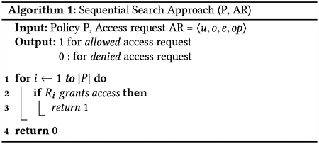
3.1. Sequentially Searching the Rules in a Policy

In ABAC, an access request can be represented as a 4-tuple: 〈u, o, e, op〉, where u ∈ U, o ∈ O, e ∈ E, op ∈ OP. In other words, a user u wants to perform operation op on the object o in environmental condition e. Whenever such an access request arrives, rules within the policy are checked sequentially, so as to find a rule which will permit the user u to perform the operation op on object o. The procedure for sequentially searching all the rules in the policy is given in Algorithm 1. We refer to this method as the sequential search approach (interchangeably, the linear search approach).

For instance, let 〈u₂, o₂, e₁, modify〉 be a requested access (ar). Consulting Tables 1–3, one can find that

$$u{v}_2=\left\{Designation=professor,Department=CSE\right\}$$

$$o{v}_2=\left\{Type=Questionpaper,Confidentiality=High\right\}$$

$$e{v}_1=\left\{Day=Weekday\right\}$$

$$op=\left\{Modify\right\}$$

Concatenating the contents of uv₂, ov₂, ev₁ and op we get:

$$\left\{Designation=Professor,Department=CSE,Type=Questionpaper,Confidentiality=High,Day=Weekday,op=Modify\right\}$$

Now, the obtained attribute-value pairs are compared with the attribute-value pairs of each of the rules. The attribute value comparisons done when the access request is sequentially evaluated against the rules in the policy are as follows:

First, the access request ar is evaluated against r₁ where it is seen that the first two attribute-value pairs in r₁ are also present in ar. The third attribute-value pair of r₁ and ar do not match. So, r₁ cannot be used by u₂ to perform the requested operation. Now, we evaluate ar against the second rule. All the six attribute-value pairs in r₂ matches with ar. Thus, r₂ permits the desired access. Since the access decision is already obtained, it is not necessary to evaluate ar against the remaining rules. The number of attribute-value pairs compared for rules r₁ and r₂ are three and six, respectively. Thus, the access request ar is resolved after a total of nine comparisons.

3.2. Rule Re-ordering for Improved Sequential Search

Now, we present a modified version of the sequential search approach which is based on re-arranging the rules of the policy and then re-shuffling the attribute-value pairs within each rule. This two-way re-ordering ensures that resolving access requests incur a lesser number of attribute-value pair comparisons as compared to the naive sequential search approach. The re-arranging procedure is given in Algorithm 2. It operates in 4 steps as discussed below.

Step 1. Prepare access data

This step (Lines 6–10 of Algorithm 2) prepares the list of all possible access requests in the ABAC system. The total number of possible access requests is |U| ×|O| ×|E| ×|OP|.

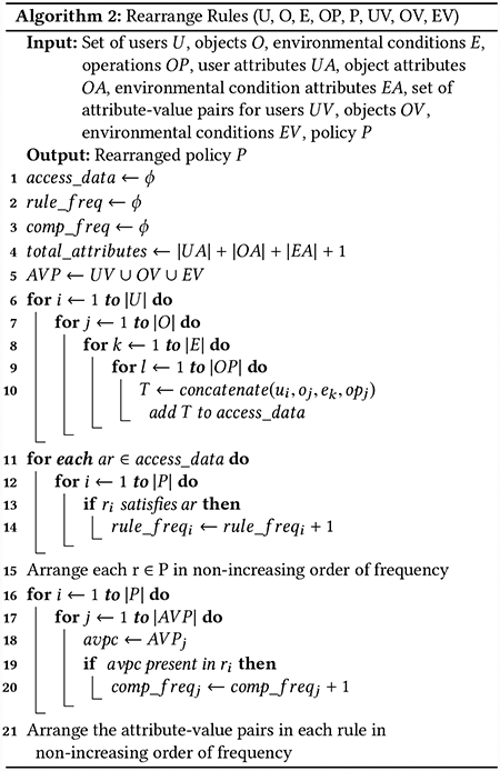
Step 2. Compute the coverage of each rule

In the second step (Lines 11–14 of Algorithm 2), the number of access requests satisfied by each rule is computed.

Step 3. Arrange the rules in the policy

In the third step (Line 15 of Algorithm 2), a re-arrangement of the rules in the policy is done in non-increasing order of the number of times a rule has been satisfied by access requests. The rule that permits most of the accesses is made the first rule of the policy. The idea behind such a re-arrangement is that an incoming access request is more likely to be satisfied by the rule that allows most number of accesses. This is based on the assumption that the access requests are uniformly distributed.

Step 4. Arrange attribute-value pairs within a rule

In the final step (Lines 16–21), the number of times an attribute-value pair occurs in the policy is computed. Then, the attribute-value pairs within each rule are re-arranged in non-decreasing order of their occurrences in the policy. This keeps the attribute-value pair with the lowest frequency at the beginning of the rule. It helps in faster discarding of a rule while resolving an access since the least frequent attribute-value pair is most unlikely to occur in an access request.

It may be noted that after re-arranging is done as an off-line onetime process, when an access request comes, the actual searching of the rules is done in a manner similar to the Baseline 1 approach mentioned above.

4. POLICY TREE FOR ABAC

The sequential search approach on the reordered rules as discussed in Sub-section 3.2 is expected to perform better than the basic sequential search approach discussed in Sub-section 3.1. However, the improvement in performance is heavily dependent on the nature of the access requests. In the worst case, its performance would be similar to that of sequential search. To address this limitation, we introduce two unique tree-based data structures for storing ABAC policies which require a lesser number of comparisons to resolve an access request.

4.1. Binary Policy Tree

In this sub-section, we present a binary tree-based data structure to store an ABAC policy. As seen in the baseline approaches discussed in the last section, comparison of attribute-value pairs is the atomic operation for resolving an access request. There are two possible outcomes for an attribute-value pair comparison, i.e., Yes (Y) or No (N). Therefore, if we consider an attribute-value pair as a node of a binary tree, resolving it automatically resolves all the attribute-value pair comparisons in all the rules where it is present.

The procedure for constructing a B-PolTree for a given ABAC policy is given in Algorithm 3 which takes as input an ABAC policy P, the set of users U, objects O, environmental conditions E as well as the three sets of attribute-value pairs, i.e., UV, OV and EV.

Each non-leaf node of B-PolTree consists of the following:

• An attribute-value pair

• Two branches, Y and N. The Y and the N branch point to the left and the right sub-trees of the current node, respectively.

Each leaf node of B − PolTree consists of the following:

• An access decision, i.e., Allow (A) or Deny (D)

B-PolTree construction requires the four steps mentioned below.

Step 1. Find the attribute-value pair with the highest number of occurrences

This step (Lines 6–7 of Algorithm 3) finds the attribute-value pair avp having the maximum normalized frequency in UV ∪ OV ∪ EV. Each attribute-value pair frequency is divided by the number of entities of the type of the attribute to obtain the normalized frequency. If multiple attribute value-pairs have the same frequency, then any one of them can be chosen randomly. A node is created with avp as its label. The attribute-value pair with the highest frequency is selected since it is more likely to occur in an access request. For example, from Tables 1 – 3 and the rules given in Section 2, Designation = Professor is the node with the highest frequency. The chosen attribute-value pair is made into a node as shown in Figure 1.

Figure 1:

Binary policy tree

Step 2. Find the rules corresponding to the selected attribute-value pair

In the second step (Lines 8–12 of Algorithm 3), two sets P_y and P_n are constructed. P_y is the set of rules in P which contain avp. P_n is the complement of P_y. avp is removed from AVP, as the same comparison will not be performed twice during the resolution of an access request. Next, for P_y and P_n, the sets S_y and S_n are created which contain the entities covered by P_y and P_n, respectively. The sets P_y, P_n, S_y and S_n corresponding to Designation = Professor are shown in Figure 1.

Step 3. Repeat the above steps with the smaller policies P_y and P_n

In the third step (Lines 13–14), Algorithm 3 is recursively invoked with the policies P_y and P_n and the new set of attribute-value pairs AVP′. This generates the left sub tree and the right sub tree of the most recently created node labeled avp.

Step 4. Create a leaf node with the only rule in the policy

This is the base condition of the recursive algorithm. In this step, if the rule set contains only a single rule, a node is created comprising the remaining attribute-value pairs of the node. Then, Y and N branches are added to the rule. Finally, leaf nodes containing A and D are added to the Y and N branch, respectively. The complete B-PolTree generated using Algorithm 3 on the example data set is shown in Figure 1.

Now, we show how an access request is resolved using the constructed B-PolTree. The algorithm for resolving an access using the B-PolTree is given in Algorithm 4, which takes a B-PolTree, an access request and the current node as inputs and returns the access decision corresponding to the requested access.

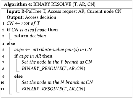
The function Binary_Resolve is initially called with the complete tree T, the incoming access request AR and the root node as the current node CN. Then the presence of the attribute-value pair of the current node is checked in the access request (Line 6). If present, the Y branch, i.e., the left branch of the current node is selected (Line 7). Otherwise, the N, i.e., the right branch is selected (Line 10). Next, the node at the end of the selected branch is set as the current node. This is continued until a leaf node is reached. Finally, the value of the leaf node is returned as the decision corresponding to the access request. The maximum number of comparisons required to resolve an access request using a B-PolTree is O(|UV| + |OV| + |EV| + |A|), where |A| is the total number attributes in the system.

4.2. N-ary Policy Tree

In this sub-section, we present another tree-based data structure for representing an ABAC policy. Here, an ABAC policy is organized in the form of an n-ary tree. We refer to the constructed tree as N-PolTree. Each non-leaf node of N-PolTree comprises:

• An attribute

• Branches for each distinct value of the attribute in the policy P

Each leaf node of an N-PolTree consists of the following:

• A node with decision A which represents allow

Algorithm 5 presents the procedure for constructing an N-PolTree that takes as input an ABAC policy P, the set of users U, objects O, environmental conditions E, operations OP and the set of all attributes, i.e., UA, OA and EA.

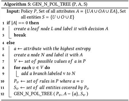
Step 1. Compute the attribute with the maximum entropy

This step (Line 5) finds the attribute with the maximum entropy. The entropy (H) of an attribute X is computed as follows:

$$H(X)=-\sum _{i=1}^{n}p\left(x_i\right)lo{g}_{2}p\left(x_i\right),$$

where x₁, x₂, …, x_n are the possible values that X can take and p(x_i) is the fraction of entities of the type to which X belongs and takes up the value x_i. p(x_i) is computed from the set of attribute-value pairs of all the entities of the same type as X. Choosing an attribute with the maximum entropy ensures that the policy is split evenly among the values that the attribute assumes in the policy P. A node is created with the selected attribute (Line 6). Next, branches corresponding to the possible values of the selected attribute are added to the created node (Lines 7–9).

For instance, considering Tables 1, 2, 3 and the rules given in Section 2, the user attribute Designation has the highest entropy. Thus, a node with the label Designation is created. Next, the two possible values of Designation, i.e., Professor and Student are added as branches of the node as shown in Figure 2.

Table 2:

Object attribute-value pair assignment

Object	Type	Confidentiality
o1	Assignment	High
o2	Question paper	High
o3	Assignment	Low
o4	Question paper	Low

Figure 2:

N-ary policy tree

Step 2. Determine the list of entities corresponding to the values of the selected attribute

In the second step (Lines 10–11 of Algorithm 5), for each branch generated in Step 1, first, the set of rules P_v is computed. P_v consists of all the rules where the value of the selected attribute is the same as the branch label. The selected attribute in Step 1 is removed from A, since the same attribute will not be compared twice during the resolution of an access request. Next, the set of entities S_v that are covered by the rules in P_v are obtained.

For example, for the branch Student in Figure 2, rules r₃ and r₆ have Designation = Student. Therefore, P_student = {r₃, r₆}. The set of users, resources and environmental conditions covered by P_student are {u₁, u₃},{o₁, o₃} and {e₂}, respectively.

Step 3. Recursively invoke the above steps with smaller policies

In the third step (Line 12), Algorithm 5 is invoked with the set of rules P_v, set of entities S_v, and the remaining set of attributes obtained in Step 2 (Line 11). This creates the remaining levels of the tree.

Step 4. Create leaf node

Finally, when all the attributes have been used up in a particular path of the policy tree and Algorithm 5 is invoked with an empty set of attributes, a leaf node with decision A is created. This is done because a path starting from the root to the leaf node represents a rule in P, and if during the resolution of an access request, the leaf node is reached, it means all the attribute-value pair comparisons in the rule have already been satisfied by the access request, and the access has to be granted. The complete N-PolTree for the illustrative example is shown in Figure 2.

After the N-PolTree construction is completed, actual evaluation of access requests can be carried out.

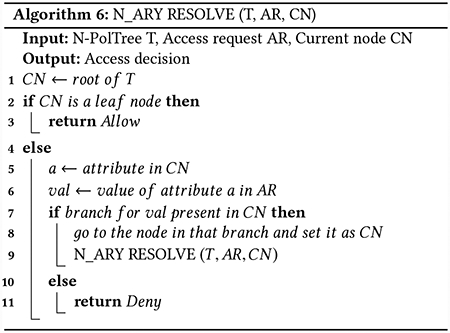
Algorithm 6 shows how an access request is resolved using the N-PolTree, where “^*” (Refer to Section 2) is not present in any of the attribute-value pairs in the ABAC policy.

Initially, the root node of the N-PolTree is set as the current node. The value corresponding to the current attribute is obtained from the access request. If the obtained value matches the label of any of the branches of the current node, the attribute in the node at the end of the selected branch is chosen and the newly reached node is set as the current node. Otherwise, if there is no branch label corresponding to the obtained value from the access request, it is denied. This procedure is repeated until the access request is denied at any node. Alternatively, if the leaf node of the N-PolTree is reached, i.e., all the attributes in the system are evaluated and there is an allowable value (branch) in the N-PolTree at every level corresponding to an attribute value in the access request, it is allowed. The maximum number of comparisons required for resolving an access request using an N-PolTree is θ(|A|), where |A| is the total number of attributes in the system.

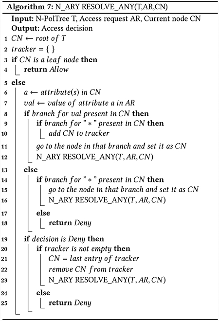
Algorithm 6 works only when no attribute in the policy is assigned the value “*”. If the value assigned to an attribute a is “^*”, the value for attribute a need not be looked for in the access request. Algorithm 7 is used to resolve an access request in a given N-PolTree where “*” is present as an attribute value in the rules of the ABAC policy.

Resolution of an access request using Algorithm 7 is similar to Algorithm 6 until an access request is denied (Lines 3–18). For resolving access requests with “*” in the policy, a list of nodes (attributes) is maintained for which there is a not yet traversed branch labeled “*”. It may sometimes occur that an access request that has been denied by the N-PolTree may be allowed if the branch corresponding to “*” is chosen instead of a branch whose label matches with the value in the access request. In such cases, Algorithm 7 falls back to the last node, i.e., to an attribute where a branch labeled “*” is present but was not traversed while resolving the access decision (Lines 19–23). If there is no node left where a branch labeled “*” is present but the branch is not traversed, the access request is finally denied (Lines 24–25).

5. EXPERIMENTAL EVALUATION

In the absence of any large scale real-life data sets, we have evaluated our proposed approaches on a number of synthetically generated data sets. Each such generated data set comprises a set of users, objects, environmental conditions, attribute-value pairs of all the entities and a policy. The proposed data structures were implemented in Python 2.7 and executed on a 3.2 GHz Intel i5 CPU having 4 GB of RAM.

We denote the obtained results using the average number of comparisons required to resolve an access for sequential search, modified sequential search, B-PolTree, and N-PolTree as C_L,C_M, C_B and C_N, respectively. We also present the speedup achieved taking sequential search as the baseline. These are denoted as S_L, S_M, S_B and S_N, respectively. Obviously, S_L = 1. The number of users, objects, environmental conditions, rules, attributes, and attribute values are denoted as |U|, |O|, |E|, ||P|, and |AV|, respectively.

For experimental evaluation, we consider variation in the average number of comparisons and speedup in the following scenarios: (i) different values of |U| and |O| (ii) different values of |P| (iii) different values of |A| and |AV|. Further, we show the impact of inclusion of “*” in the data sets and compare the performance of B-PolTree and N-Poltree for the following situations: (i) different values of |P| (ii) different values of |A| and |AV|. Since the data sets are synthetically generated, the number of attribute-value pair comparisons and speedup presented in this section are computed as the average of 1000 cases. We have rounded off the average number of comparisons in each instance to the nearest integer.

Table 4 shows the variation in the average number of comparisons required to resolve an access request as well as the speedup for the two baseline approaches and the two tree-based approaches for different number of users and objects. Little variation is observed in the average number of comparisons required to resolve an access request for each of the proposed approaches. This is attributed to the fact that the number of comparisons is independent of the number of users and objects in the system. In this situation, N-PolTree performs the best among all the approaches followed by B-PolTree. The difference in performance of B-PolTree and N-PolTree is because in N-PolTree, the maximum number of comparisons required to resolve an access request is O(|A|), where |A| is the number of attributes. For B-PolTree, it is O(|AV|), where |AV| is the total number of possible attribute-value pairs. The modified sequential search approach performs marginally better than Baseline 1. Performance of the tree-based approaches clearly surpasses both the baselines. A similar trend is observed in the speedup of the proposed approaches. N-PolTree clearly edges past B-PolTree, followed by the two baselines. This trend is due to the fact that the time required to resolve an access is dependent on the number of comparisons made.

Table 4:

Variation in the average number of comparisons required to resolve an access and speedup for different number of users and objects

|E| = 10, |P| = 100, |A| = 10, |AV| = 10
	|O| = 100								|O| = 200
|U|	CL	SL	CM	SM	CB	SB	CN	SN	CL	SL	CM	SM	CB	SB	CN	SN
100	116	1	103	1.56	10	11.11	5	14.28	115	1	105	1.96	10	12.08	4	19.00
200	114	1	105	1.81	9	10.00	4	20.00	121	1	102	1.84	9	11.59	4	17.88
500	118	1	106	1.61	10	11.11	5	16.67	116	1	109	1.53	11	11.04	5	20.13

	|O| = 500								|O| = 1000
|U|	CL	SL	CM	SM	CB	SB	CN	SN	CL	SL	CM	SM	CB	SB	CN	SN
100	115	1	104	1.63	11	12.26	5	16.34	117	1	103	1.88	11	11.76	5	20.22
200	117	1	108	1.91	10	11.50	5	18.58	119	1	110	1.97	10	12.63	5	16.67
500	120	1	107	1.56	10	11.74	5	15.33	118	1	105	1.64	10	11.44	4	19.48

Table 5 shows the variation in average number of comparisons required to resolve an access request and the speedup for all the four approaches proposed in Sections 3 and 4 for different policy sizes. The average number of comparisons required for resolving an access using all the approaches, barring N-PolTree, increases with the number of rules. For the two baseline approaches, as all the rules are sequentially evaluated to resolve an access request, the increase in the number of comparisons is justified. For B-PolTree, each node is split unless there is only one rule corresponding to an attribute-value pair. Thus, for more number of rules, the height of B-PolTree increases, which results in more number of comparisons. N-PolTree outperforms all the other approaches once again. This is attributed to the fact that the number of comparisons for resolving an access request using N-PolTree is dependent only on the number of attributes. A similar trend is observed in speedup of the proposed approaches, where N-PolTree has better performance due to lesser number of comparisons required with respect to the other approaches.

Table 5:

Variation in the average number of comparisons required to resolve an access and speedup for different policy sizes

|U| = 100, |O| = 1000, |E| = 10, |A| = 10, |AV| = 10
|P|	CL	SL	CM	SM	CB	SB	CN	SN
10	17	1	13	1.61	7	1.96	5	2.56
50	60	1	52	1.56	9	5.88	3	16.67
100	115	1	104	1.51	11	11.11	4	25.00
500	553	1	523	1.35	18	42.23	4	138.25
1000	1109	1	1051	1.35	20	76.76	4	277.25

In Table 6, we show the effect of varying the number of attributes and their possible values on the average number of comparisons to resolve an access and also on speedup. For the two baseline approaches, the number of accesses required to resolve an access increases with the number of attributes. However, marginal change is seen for increase in the number of attribute values. This is attributed to the fact that in both the baseline approaches, the maximum number of comparisons to resolve an access is O(|P| × |A|), where |P| and |A| are the number of rules and attributes, respectively. In B-PolTree, the average number of comparisons required increases only with the number of attributes. This is due to the fact that the number of comparisons required to evaluate a rule increases with the number of attributes in the system. Here too, N-PolTree performs better than the rest of the approaches. As the number of attribute values simply increases the number of branches a node can have, it does not affect the number of comparisons. We select the required branch using a hash table in O(1). However, the number of comparisons required increases with the number of attributes. Similar to Tables 4 and 5, the speedup in resolving an access varies uniformly with the average number of comparisons.

Table 6:

Variation in the average number of comparisons required to resolve an access and speedup for different number of attributes and possible attribute values

|U| = 100, |O| = 1000, |E| = 10, |P| = 10
	|AV| = 2								|AV| = 5
|A|	CL	SL	CM	SM	CB	SB	CN	SN	CL	SL	CM	CM	CB	SB	CN	SN
5	70	1	57	1.34	8	8.27	5	13.59	67	1	55	1.24	10	6.97	6	11.52
10	118	1	108	1.11	17	6.85	10	11.34	116	1	103	1.13	15	7.24	9	13.19
20	227	1	211	1.15	23	9.74	13	17.95	231	1	204	1.18	22	9.89	14	16.78

|AV| = 10
|A|	CL	SL	CM	SM	CB	SB	CN	SN
5	76	1	61	1.26	8	9.24	5	15.47
10	118	1	106	1.21	12	10.25	7	16.46
20	229	1	208	1.19	21	10.47	13	17.87

Next, we present results involving data sets that have “*” as a possible attribute value. Since the tree-based approaches are bound to perform better than the baseline approaches, we present the following results considering only the two tree-based approaches for the sake of brevity. The speedup presented in the results to follow is computed with respect to the average number of comparisons required to resolve an access with the N-PolTree approach.

Table 7 shows the variation in the average number of comparisons and speed up for resolving an access for different number of rules. It is seen that B-PolTree performs better than N-PolTree. This is owing to the fact that, in B-PolTree, if a leaf node labeled Deny is reached, the access is resolved. On the other hand, in N-PolTree, it is required to return to the previous nodes and traverse the branches labeled “*” for initially denied access requests. This increase in the number of rules results in more number of attributes being assigned the value “*”, which increases the number of branches labeled “*”. It leads to repeated back-tracking to the *-labeled branches for the apparently denied access. Thus, the average number of comparisons required to resolve an access request using N-PolTree increases with the number of rules. This makes B-PolTree a suitable choice for situations where there are many attributes having the value “*” in the rules. The speedup is seen to be in accordance with the required number of comparisons.

Table 7:

Variation in the average number of comparisons required to resolve an access and speedup for different policy sizes for data sets having *

|U| = 100, |O| = 1000, |E| = 10, |A| = 10, |AV| = 10
|P|	CB	SB	CN	SN
10	6	1.38	9	1
50	10	2.57	31	1
100	13	3.48	44	1
500	18	4.05	61	1
1000	24	4.33	81	1

Table 8 shows the variation in the average number of comparisons and speedup for different number of attributes and the number of attribute values. Similar to Table 6, the average number of comparisons required to resolve an access increases with the number of attributes for both B-PolTree and N-PolTree. Similar to Table 7, B-PolTree performs better than N-PolTree due to the overhead incurred by N-PolTree in back-tracing and traversing *-labeled branches when required.

Table 8:

Variation in the average number of comparisons required to resolve an access and speedup for different number of attributes and possible attribute values for data sets having *

|U| = 100, |O| = 1000, |E| = 10, |P| = 100
	|AV| = 2				|AV| = 5				|AV| = 10
|A|	CB	SB	CN	SN	CB	SB	CN	SN	CB	SB	CN	SN
5	10	2.67	23	1	9	2.89	27	1	9	3.65	31	1
10	18	2.29	37	1	16	2.12	41	1	10	3.72	38	1
20	22	2.59	53	1	24	2.53	58	1	23	2.35	52	1

6. RELATED WORK

In the context of deployment of ABAC in organizations, there is some existing work on standardization [12], policy engineering [18] [10] [23] [9], etc. Moreover, procedures have been developed for enabling organizations to migrate to ABAC from other access control models [14]. There is, however, no existing work on efficient evaluation of ABAC rules for resolving access requests.

It may be noted that, the nature of the work presented in this paper has some similarity with the maintenance and evaluation of firewall policies. Prior work pertaining to firewall policy management includes representation of firewall policies using decision trees [17]. There is also selected work on representing firewall policies using tree-based data structures [1], improving the speed of firewall policy verification [15] and the use of boolean satisfiability for firewall policy analysis [13]. Further, there is some existing work that develops a unified index for efficient enforcement of spatiotemporal authorizations [3, 4].

However, to the best of our knowledge, there is no work which is aimed at improving the performance of ABAC once it has been deployed in an organization. The B-PolTree proposed by us is similar in structure to an Ordered Binary Decision Diagram (OBDD) [2]. But the similarity ends there. Usually, OBDDs are used for representing boolean expressions [16], synthesizing circuits [5] and formal verification [6]. There is also work that enables fast distributed evaluation of ABAC policies [7], but the main goal there is to reduce the number of communication messages and thus achieve low latency.

The basic structure of N-PolTree is loosely based on that of decision trees [19]. However, decision trees are used as tools for classification [20] and prediction [21]. Despite the structural similarity, the usage of N-PolTree in our work is completely different. Additionally, the procedure for resolving an access request using an N-PolTree is evidently distinct from that of a decision tree.

7. CONCLUSION AND FUTURE WORK

In this paper, we have introduced two tree-based data structures, namely, B-PolTree and N-PolTree, which can significantly improve the performance of ABAC in an organization by facilitating fast resolution of access requests. We have also provided extensive results that show the robustness of the proposed data structures. Future work in this area would include dynamically updating the nodes of B-PolTree and N-PolTree based on incoming access requests over a period of time for further reducing the time and number of comparisons required to resolve an access.

CCS CONCEPTS.

• Security and privacy → Access control.

REFERENCES

- [1].Al-Shaer ES and Hamed HH. 2003. Firewall policy advisor for anomaly discovery and rule editing. In International Symposium on Integrated Network Management 17–30. [Google Scholar]
- [2].Andersen HR. 1997. An introduction to binary decision diagrams Lecture notes, available online, IT University of Copenhagen; (1997). [Google Scholar]
- [3].Atluri V and Guo Q. 2005. Unified Index for Mobile Object Data and Authorizations. In Computer Security - ESORICS 2005, 10th European Symposium on Research in Computer Security, Milan, Italy, September 12–14, 2005, Proceedings. 80–97. 10.1007/11555827_6 [DOI] [Google Scholar]
- [4].Atluri V, Guo Q, Shin H, and Vaidya J. 2010. A unified index structure for efficient enforcement of spatiotemporal authorisations. IJICS 4, 2 (2010), 118–151. 10.1504/IJICS.2010.034814 [DOI] [Google Scholar]
- [5].Berman CL. 1989. Ordered binary decision diagrams and circuit structure. In IEEE International Conference on Computer Design: VLSI in Computers and Processors 392–395. 10.1109/ICCD.1989.63394 [DOI] [Google Scholar]
- [6].Bryant RE. 1995. Binary decision diagrams and beyond: Enabling technologies for formal verification. In IEEE/ACM international conference on Computer-aided design IEEE Computer Society, 236–243. [Google Scholar]
- [7].Bui T, Stoller SD, and Sharma S. 2017. Fast distributed evaluation of stateful attribute-based access control policies. In IFIP Annual Conference on Data and Applications Security and Privacy Springer, 101–119. [Google Scholar]
- [8].Das S, Mitra B, Atluri V, Vaidya J, and Sural S. 2018. Policy Engineering in RBAC and ABAC. 24–54.
- [9].Das S, Sural S, Vaidya J, and Atluri V. 2018. HyPE: A Hybrid Approach toward Policy Engineering in Attribute-Based Access Control. IEEE Letters of the Computer Society (2018), 25–29. [DOI] [PMC free article] [PubMed] [Google Scholar]
- [10].Das S, Sural S, Vaidya J, and Atluri V. 2018. Using Gini Impurity to Mine Attribute-based Access Control Policies with Environment Attributes. In ACM Symposium on Access Control Models and Technologies 213–215. [DOI] [PMC free article] [PubMed] [Google Scholar]
- [11].Hu V, Ferraiolo DF, Kuhn DR, Kacker RN, and Lei Y. 2015. Implementing and Managing Policy Rules in Attribute Based Access Control. In IEEE International Conference on Information Reuse and Integration 518–525. [Google Scholar]
- [12].Hu VC, Ferraiolo D, Kuhn DR, Schnitzer A, Sandlin K, Miller R, and Scarfone K. 2014. Guide to Attribute-Based Access Control (ABAC) definition and considerations Technical Report. NIST Special Publication; 800–162. http://nvlpubs.nist.gov/nistpubs/-specialpublications/NIST.sp.800-162.pdf [Google Scholar]
- [13].Jeffrey A and Samak T. 2009. Model Checking Firewall Policy Configurations. In IEEE International Symposium on Policies for Distributed Systems and Networks 60–67. [Google Scholar]
- [14].Jin X, Krishnan R, and Sandhu R. 2012. A Unified Attribute-Based Access Control Model Covering DAC, MAC and RBAC In Data and Applications Security and Privacy, Cuppens-Boulahia N, Cuppens F, and Garcia-Alfaro J (Eds.). 41–55. [Google Scholar]
- [15].Khummanee S and Tientanopajai K. 2016. The Policy Mapping Algorithm for High-speed Firewall Policy Verifying. International Journal of Network Security (2016), 433–444. [Google Scholar]
- [16].Liaw H and Lin C. 1992. On the OBDD-representation of general Boolean functions. IEEE Trans. Comput (1992), 661–664. [Google Scholar]
- [17].Liu Alex X.. 2009. Firewall Policy Verification and Troubleshooting. Computer Networks: The International Journal of Computer and Telecommunications Networking (2009), 2800–2809. [Google Scholar]
- [18].Narouei M, Khanpour H, Takabi H, Parde N, and Nielsen R. 2017. Towards a Top-down Policy Engineering Framework for Attribute-based Access Control. In ACM Symposium on Access Control Models and Technologies 103–114. [Google Scholar]
- [19].Quinlan JR. 1986. Induction of decision trees. Machine learning 1, 1 (1986), 81–106. [Google Scholar]
- [20].Safavian SR and Landgrebe D. 1991. A survey of decision tree classifier methodology. IEEE transactions on systems, man, and cybernetics (1991), 660–674. [Google Scholar]
- [21].Song Y and Ying L. 2015. Decision tree methods: applications for classification and prediction. Shanghai archives of psychiatry (2015), 130–135. [DOI] [PMC free article] [PubMed] [Google Scholar]
- [22].Xu Z and Stoller SD. 2014. Mining attribute-based access control policies from logs. In IFIP Annual Conference on Data and Applications Security and Privacy Springer, 276–291. [Google Scholar]
- [23].Xu Z and Stoller SD. 2015. Mining Attribute-Based Access Control Policies. IEEE Transactions on Dependable and Secure Computing (2015), 533–545. [Google Scholar]