Gene expression across mammalian organ development

Abstract

The evolution of gene expression in mammalian organ development remains largely uncharacterized. Here we report the transcriptomes of seven organs (cerebrum, cerebellum, heart, kidney, liver, ovary and testis) across developmental time points from early organogenesis to adulthood for human, macaque, mouse, rat, rabbit, opossum and chicken. Comparisons of gene expression patterns identified developmental stage correspondences across species, and differences in the timing of key events during the development of the gonads. We found that the breadth of gene expression and the extent of purifying selection gradually decrease during development, whereas the amount of positive selection and expression of new genes increase. We identified differences in the temporal trajectories of expression of individual genes across species, with brain tissues showing the smallest percentage of trajectory changes, and the liver and testis showing the largest. Our work provides a resource of developmental transcriptomes of seven organs across seven species, and comparative analyses that characterize the development and evolution of mammalian organs.

Understanding the molecular evolution of mammalian phenotypic traits is a fundamental biological goal. To achieve it, evolutionary studies need to be conducted within a developmental framework, both because adult phenotypes are defined during development^1–3 and because evolutionary and developmental processes are intertwined. von Baer noted in the 19^th century that morphological differences between species increase as development advances⁴ and evidence for it has accumulated^4,5. Understanding the molecular foundations of these patterns will facilitate the identification of general principles underlying phenotypic evolution.

Here we provide a resource of bulk transcriptomes across developmental stages, covering multiple organs from early organogenesis to adulthood in seven species, enabling direct comparisons of expression patterns in organ development within and across mammals (http://evodevoapp.kaessmannlab.org). This resource enabled us to analyse the evolution of gene expression within mammalian organs across developmental stages.

Organ developmental transcriptomes

We generated gene expression time series (RNA-seq) for six mammals (human, rhesus macaque, mouse, rat, rabbit, opossum) and a bird (red junglefowl, henceforth “chicken”). We sampled seven organs representing the three germ layers: brain (forebrain/cerebrum) and cerebellum (hindbrain/cerebellum) (ectoderm); heart, kidney, ovary and testis (mesoderm); and liver (endoderm) (Fig. 1a). The time series span from early organogenesis to adulthood, plus senescence in primates. We sampled prenatal development at regular intervals (e.g., daily in rodents, weekly in humans), and postnatally we sampled neonates, “infants”, juveniles, and adults (Fig. 1). There are exceptions: we lack early prenatal data for rhesus and chicken, and ovary data for rhesus and postnatal human development (Supplementary Table 1). Because marsupial organ development occurs predominantly postnatally⁶, all sampled stages except for one were collected postnatally. The dataset consists of 1,893 libraries (Supplementary Table 2).

Figure 1 |. Organ developmental transcriptomes.

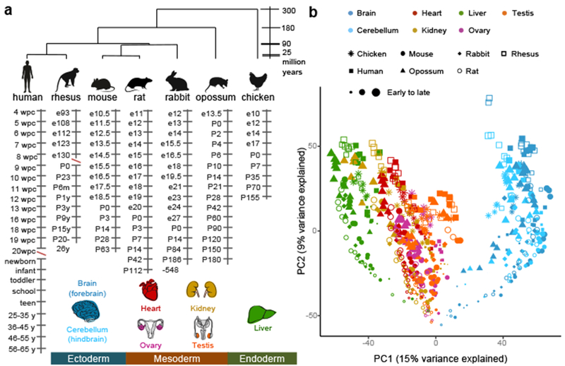
a, Species, organs, and stages sampled. Red slashes highlight two sampling gaps: human development is not covered between 20 and 38 weeks post-conception (wpc) and rhesus development between embryonic (e) day 130 and e160. b, PCA based on 7,696 1:1 orthologs across all species. Each dot represents the median across replicates (~2-4).

The global relationships among all samples can be explored through a principle component analysis (PCA) (Fig. 1b). The first principal component (PC1), explaining most variance in gene expression, separates the samples by the germ layer from which organs originate. PC2 separates the samples by developmental stage (from early to late development). PC3 and PC4 separate the samples by species (Extended Data Fig. 1a). In PCAs of individual organs, PC1 and PC2 order the samples by developmental stage and separate them by species (Extended Data Fig. 1b). In the global PCA (Fig. 1b), the earliest samples from different organs cluster together, suggesting strong commonalities. We hypothesized that developmental programs are still largely shared across organs at these early stages and found that organ transcriptomes are indeed most similar at these stages (Extended Data Fig. 1c). Throughout development, the expression of transcription factors (TFs) differs more between organs than that of the whole transcriptome (Extended Data Fig. 1c), consistent with TFs directing organogenesis.

Next, we identified genes with significant temporal expression changes in each organ, termed developmentally dynamic genes (DDGs; Extended Data Fig. 2a; Supplementary Tables 3–9; Methods). DDGs reflect changes during development in gene regulation, cell type abundance, and/or the proportion of cells undergoing division¹. Consistently, between 79-91% of protein-coding genes in each species are DDGs (Extended Data Fig. 2b), including genes with housekeeping functions. DDGs are enriched with phenotypes associated with the development, anatomy and physiology of each organ, plus general growth and patterning (FDR < 0.01, hypergeometric test; Supplementary Tables 10–11). DDGs are under stronger functional constraints^7–10 than non-DDGs, and the constraints increase with the number of organs in which genes show temporal dynamic expression (Extended Data Fig. 2c). The increased constraints extend to dosage changes, with DDGs being less tolerant to duplication and deletion variants¹¹ (Extended Data Fig. 2d).

In each species, 6-15% of the genes (Extended Data Fig. 2b) are DDGs in only one organ, and are consistently enriched with organ-specific phenotypes (FDR < 0.01, hypergeometric test; Supplementary Table 12). The fraction of expressed organ-specific DDGs increases during development (Extended Data Fig. 2e), correlating with organ differentiation and maturation. The opposite is observed for TFs, whose contribution is highest earlier in development (Extended Data Fig. 2f).

Developmental correspondences and heterochrony

Embryonic development is divided into 23 Carnegie stages, which are matched across species^12–15 (Extended Data Fig. 3a). However, cross-species correspondences during fetal and postnatal development are unknown. Therefore, we used the developmental transcriptomes to establish stage correspondences across species throughout the entire development (Methods; Fig. 2a; Extended Data Fig. 3b). We recapitulated the Carnegie stage correspondences (rabbit is shifted 1-2 days; Methods; Extended Data Fig. 3a) and found that gene expression in a newborn opossum is closest to a mouse at e11.5, matching previous estimates¹⁶.

Figure 2 |. Developmental correspondences.

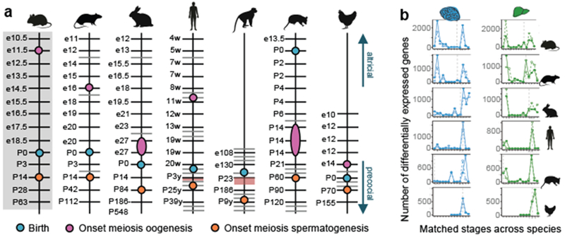
a, Stage correspondences across species. Grey bars represent additionally sampled stages. Red shading highlights sampling gaps. In rhesus, male meiosis starts at 3-4 years³⁶. Because we did not detect expression of meiotic genes in the 3-year-olds, we placed meiosis’ onset between 3 and 9 years. c, Number of genes differentially expressed between adjacent, species-matched, stages for brain and liver (log₂ fold-change ≥ 0.5; other organs in Extended Data Fig. 5). Solid lines mark genes that increase in expression and dashed lines genes that decrease. Vertical dotted line marks birth.

Organ development includes periods of greater transcriptional change¹⁷. We identified and characterized these periods across species using our stage correspondences. These periods occur at similar stages across species and are enriched with orthologous genes (P ≤ 0.001, hypergeometric test; Fig. 2b; Extended Data Figs. 4, 5). In somatic organs, there are two main periods of transcriptional change. The first occurs during embryonic development and is defined by an increase in expression of genes with early organ-specific functions and a decrease in expression of genes involved in cell division and general morphogenesis (Fig. 2b; Extended Data Figs. 4, 5; Supplementary Table 13). The second occurs either postnatally or around birth, depending on the maturity of the newborns of the different species. Mammals exhibit great variability in their level of independence at birth, being classified as altricial (born less mature) or precocial (more mature)⁶. These classifications are recapitulated by the developmental transcriptomes, with the altricial newborn opossum at one end of the maturation spectrum and the precocial rhesus macaque at the other (Fig. 2a). This second period of greater transcriptional change is defined by an increase in expression of genes with late organ-specific functions and, again, by a decrease in expression of genes involved in cell division and morphogenesis (Fig. 2b; Extended Data Figs. 4, 5; Supplementary Table 13). Thus, whereas in altricial species this period of intense organ maturation occurs postnatally, in precocial species it overlaps with birth.

Developmental programs can change through shifts in the timing of events, i.e. “heterochrony”¹. If the development of an organ were to be shifted in one species, the developmental correspondences for that organ would be different from the global correspondences. Overall, organ-specific correspondences are consistent with the global correspondences, except for early heart development in opossum and early ovary development in human and rabbit (Extended Data Fig. 6; Methods).

However, heterochronies do not have to involve whole organs, they can occur in developmental modules within organs. Indeed, heterochronies occur during the production of gametes¹⁸, a process dependent on meiosis. Stra8 is the gatekeeper for germ cell entry into meiosis and its role is conserved across vertebrates^3,19. Therefore, we analyzed the expression of Stra8 and other meiotic genes to identify the start of meiosis in each species, and identify differences in its timing across species (Fig. 2a; Extended Data Figs. 7a–d). During oogenesis, meiotic genes are expressed as early as during embryonic development (mouse), at the boundary between embryonic and fetal development (rat and human), or during late fetal development (rabbit) (Fig. 2a; Extended Data Figs. 6, 7a–b). Although less frequent, we also identified heterochronies in the onset of meiosis during spermatogenesis (Fig. 2a; Extended Data Fig. 7c–d). In spermatogenesis the onset of meiosis marks the beginning of dramatic changes in cellular composition²⁰, which sharply change testis transcriptomes (Extended Data Fig. 7e). Starting at birth in rodents and later in rabbit there are also profound changes in ovary transcriptomes (Extended Data Fig. 7e), coinciding with the breakdown of germ cell nests and follicle assembly²¹. Heterochronies are therefore abundant during mammalian gonadal development, representing another mechanism underlying the extreme variability of gonadal morphogenesis³.

Relationships between evolution and development

After the phylotypic period, the most conserved embryonic stage, morphological differences between species increase as development progresses — von Baer’s divergence^4,5 (Extended Data Fig. 8a). Previous studies assessed the relationship between development and molecular divergence for whole embryos and found that molecular divergence increases as development progresses^22–25. We recapitulated this observation for individual organs, consistently finding transcriptome correlations between species to decline with developmental time (Extended Data Fig. 8b).

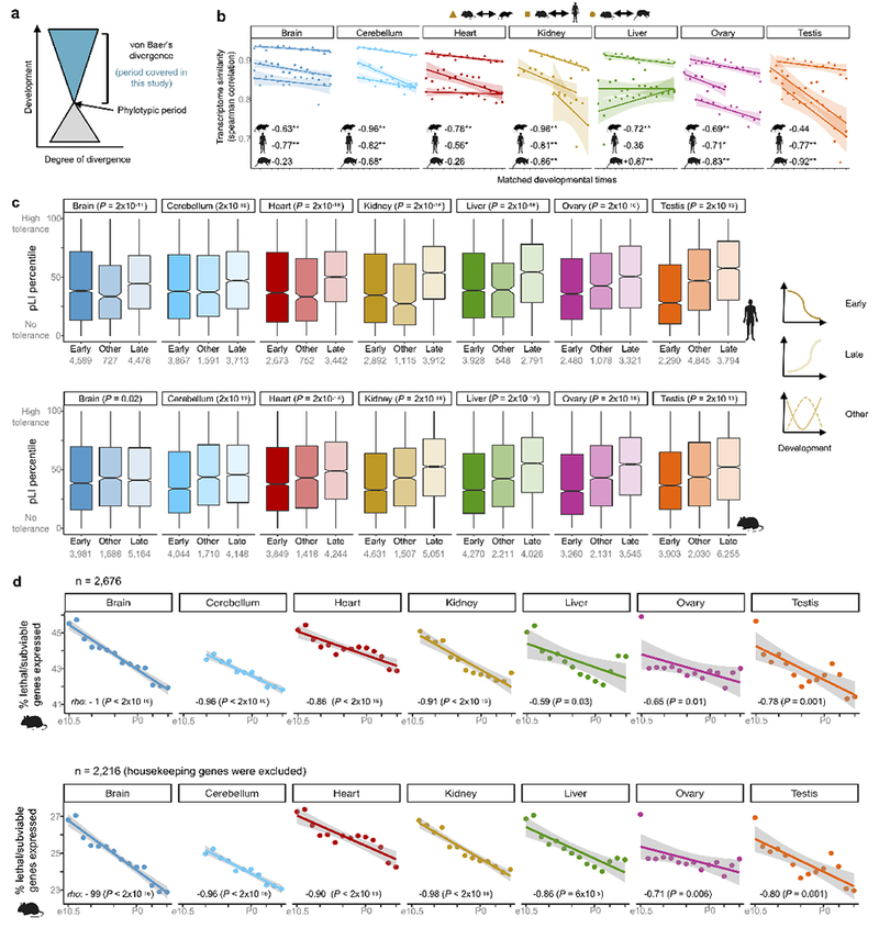
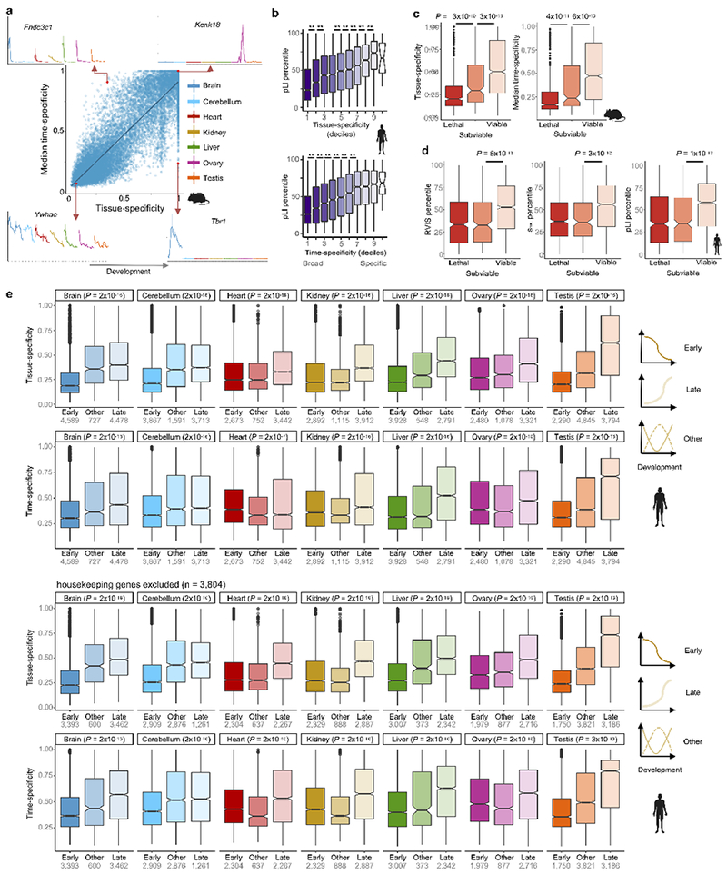
Two non-mutually-exclusive hypotheses can account for the increasing molecular and morphological divergence during development²⁶. First, early development could be under greater functional constraints and be more refractory to change. Second, divergence could be driven by adaptive changes, which are more likely to occur later in development, when the influence of the environment is stronger²⁶. To assess potential differences in functional constraints across development, we compared the tolerance to functional mutations of genes employed in early versus late development. Across all organs, genes employed early in development are less tolerant to loss-of-function mutations (P < 10⁻¹⁰, Wilcoxon rank sum test, two-sided; Fig. 3a; Extended Data Fig. 8c). Consistently, using a set of neutrally ascertained mouse knockouts²⁷, we observed for all organs that the percentage of expressed genes associated with lethality decreases during development (Fig. 3b; Extended Data Fig. 8d). Both observations suggest that early development is subject to stronger functional constraints. Next, we evaluated the relationship between adaptation and development by examining the temporal expression of genes identified as carrying signatures of positive selection²⁸. Organs differ in the proportion of positively selected genes: it is highest in liver and testis and lowest in brain tissues (Fig. 3c). However, across all organs, the fraction of expressed positively selected genes increases during development (Fig. 3c). Thus, an increase in positive selection likely also contributes to the progressive molecular and morphological divergence of organs during development.

Figure 3 |. Relationships between evolution and development.

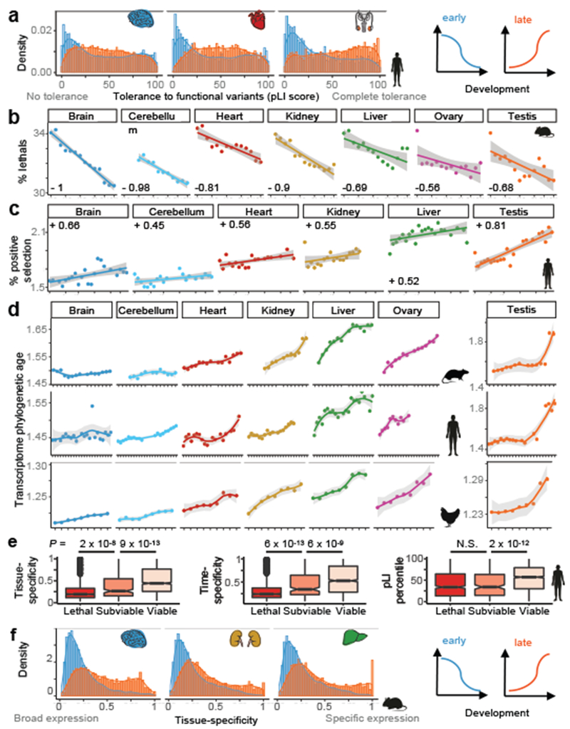
a, Intolerance to functional mutations (pLI) for human genes whose expression decreases (blue) or increases (orange) during development (4,589/4,478 genes decrease/increase in brain, 2,673/3,442 in heart, and 2,290/3,794 in testis; all P < 10⁻¹⁰, Wilcoxon rank sum test, two-sided). b, Percentage of lethal genes expressed at each stage (out of 2,676 knockouts). Weighted average Spearman correlation coefficient is −0.89 (P = 1 × 10⁻¹²); all organ-specific Spearman correlations are significant (P ≤ 0.04). c, Percentage of positively-selected genes expressed at each stage (out of 13,362 genes tested for positive selection). Ovary excluded due to lack of postnatal data. Weighted average Spearman correlation coefficient is +0.57 (P = 5 × 10⁻¹¹); all organ-specific correlations are significant (P ≤ 0.05). d, Phylogenetic age of organs’ transcriptomes throughout development for rat (n = 18,695 genes), human (n = 18,820) and chicken (n = 15,155). Higher values indicate larger contributions of lineage-specific genes (i.e. younger transcriptomes). Weighted average Spearman correlation coefficients are +0.87 (P = 1 × 10⁻¹²) for rat, +0.77 (P = 1 × 10⁻¹²) for human and +0.96 (P = 1 × 10⁻¹²) for chicken. All Spearman correlations are significant except for rat brain and cerebellum (ρ: +0.53 to +0.99, P: 0.03 to 10⁻¹⁵). Testis plotted separately because of the young age of sexually mature transcriptomes. e, Tissue-specificity, time-specificity (median across organs) and intolerance to functional mutations (pLI) of human orthologs of mouse genes identified as lethal, subviable and viable (n = 2,686; Wilcoxon rank sum test, two sided; ‘N.S.’ means non-significant). Box plots depict the median ± 25th and 75th percentiles, whiskers at 1.5 times the interquartile range. f, Tissue-specificity for mouse genes whose expression decreases (blue) or increases (orange) during development (3,981/5,164 genes decrease/increase in brain, 4,631/5,051 in kidney, and 4,270/4,026 in liver; all P < 10⁻¹⁵, Wilcoxon rank sum test, two-sided). In b-d, the x-axes show samples ordered by stage (Fig. 1a). In b-c, lines were estimated through linear regression; in d through loess. In b-d the 95% confidence interval is shown in grey.

Organ transcriptomes can also diverge between species due to species-specific genes²⁹. Therefore, we investigated how the contribution of recent gene duplications changes throughout development. For each stage, we calculated an index combining the phylogenetic age of genes with their expression, where higher values correspond to younger transcriptomes (Methods). We identified differences between organs similar to those observed for positively selected genes: liver has the youngest developmental transcriptomes, brain tissues the oldest (Fig. 3d). However, across organs, transcriptomes become younger during development, indicating that gene duplications play increasingly more prominent roles (Fig. 3d).

Together, these analyses suggest that the increase in morphological and molecular divergence observed between species during development is driven by a decrease in functional constraints as development advances (Figs. 3a–b), and by a concurrent increase in positive selection (Fig. 3c) and addition of new genes (Fig. 3d).

Pleiotropy and the evolution of development

The breadth of expression across tissues and timepoints (which we refer to here as pleiotropy) has an influence on gene evolution^30,31. Therefore, we calculated the tissue- and time-specificity of each gene across development (Extended Data Fig. 9a; Methods; Supplementary Tables 3–9). Time- and tissue-specificity are highly correlated: tissue-specific genes are more likely to be expressed in narrower time windows and vice versa (Pearson correlation coefficients, r: 0.63-0.89, P < 10⁻¹⁵). Genes also tend to have similar temporal breadths across organs (r: 0.48-0.92, P < 10⁻¹⁵). As described^32,33, pleiotropy correlates with levels of functional constraint: the more broadly expressed, the more intolerant genes are to functional variation (r = 0.29, P < 10⁻¹⁵; Extended Data Fig. 9b). Consistently, genes associated with lethality²⁷ are more broadly expressed than genes associated with subviability, which in turn are more broadly expressed than genes associated with viability (all P ≤ 2 × 10⁻⁸, Wilcoxon rank sum test, two-sided; Fig. 3e; Extended Data Fig. 9c). This contrast with measures of tolerance to functional mutations, which distinguish genes associated with lethality or subviablity from viability (P = 2 × 10⁻¹²), but do not differentiate between lethality and subviability (Fig. 3e; Extended Data Fig. 9d). Expression pleiotropy is therefore uniquely correlated with phenotypic impact.

Pleiotropy has been forwarded as an explanation for the conservation of the phylotypic period^24,34 and is a determinant of the types of mutations that are permissible under selection^30,31. Therefore, we tested for differences in pleiotropy between genes employed early versus late in development and found that genes employed earlier have broader spatial and temporal expression than genes employed later (all P < 10⁻⁶, Wilcoxon rank sum test, two-sided; Fig. 3f; Extended Data Fig. 9e). Because a decrease in pleiotropy can explain both a decrease in functional constraints and an increase in adaptation^30,31, we suggest that it may be a major contributor to the increase in morphological and molecular divergence observed between species during development.

Evolution of developmental trajectories

Differences between species in organ development are often correlated with changes in gene expression. Consequently, we sought to identify genes that evolved new developmental trajectories. Hence, we compared, within a phylogenetic framework, the temporal profiles of orthologous DDGs and identified those with trajectory changes between species (Fig. 4a, b; Supplementary Tables 14–18; Methods).

Figure 4 |. Evolution of developmental trajectories.

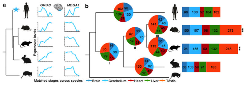
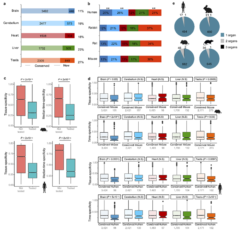
a, Example of two genes that evolved new trajectories in the human cerebellum. GRIA3 is a glutamate receptor associated with mental retardation. MDGA1 encodes a cell surface glycoprotein important for the developing nervous system. b, Pie charts depict the number of genes in each organ that evolved new trajectories in each phylogenetic branch (3,980 genes tested in brain, 3,064 in cerebellum, 1,871 in heart, 2,284 in liver and 3,191 in testis). Bar charts depict the total number of trajectory changes in each species. For mouse, that meant adding the changes that occurred at the base of the glires (I), those shared by mouse and rat (II) and those that are mouse specific (III). **P < 10⁻¹⁰, binomial test.

Brain exhibits the smallest percentage of trajectory changes (11% DDGs), liver and testis the highest (23% and 27%, respectively; Extended Data Fig. 10a). These organ differences are consistent with those observed for positively selected genes and for gene duplications. Thus, across all evaluated mechanisms of evolutionary change, the brain is the slowest evolving organ, whereas liver and testis are the fastest.

In mouse, rat and rabbit the distribution of trajectory changes among organs is similar (Extended Data Fig. 10b). Compared to these species, humans display an excess of trajectory changes in brain (20% changes in human vs. 12-13% in others; P = 1 × 10⁻⁵, binomial test) and cerebellum (26% in human vs. 21-22% in others; P = 0.02), and a paucity in testis (21% in human vs. 34-37% in others; P = 1 × 10⁻¹⁰) (Extended Data Fig. 10b). Although it is tempting to invoke adaptation, the excess of changes in the human brain tissues could partly stem from differences in sampling (Methods). Overall, rodents evolved a higher number of trajectory changes when compared to human and rabbit (P < 10⁻¹⁰; Fig. 4b).

Orthologs tested for trajectory changes are more pleiotropic than the full set of genes in each species, which also includes gene duplications/losses (all P < 10⁻¹², Wilcoxon rank sum test, two-sided; Extended Data Fig. 10c). However, among those tested, genes with new trajectories are as pleiotropic as genes with conserved trajectories (Extended Data Fig. 10d). Importantly, while genes with trajectory changes are broadly expressed, the changes themselves are organ-specific (Extended Data Fig. 10e). Trajectory changes are restricted to one organ in 93-96% of the cases. This is consistent with the underlying mutations affecting regulatory elements, which control a subset of the total spatiotemporal profile of each gene, and with evolutionary theory, as mutations affecting multiple organs are less likely to fix in populations^30,31. However, not all trajectory changes are directly due to regulatory mutations; they can also be caused by changes in cellular composition.

Discussion

We profiled the development of seven major organs, from early organogenesis to adulthood, across multiple mammals, to create an extensive resource (evodevoapp.kaessmannlab.org). We used developmental transcriptomes to match stages across species and identified extensive heterochronies during gonadal development. We found the evolution of mammalian organs to be inextricably linked to their development. Organs are most similar between species early in development and then become increasingly more distinct, which is likely explained by changes in pleiotropy during development. Early in development, active genes tend to function in multiple organs and stages, rendering them more refractory to change. As organs differentiate and mature, active genes have more restricted spatiotemporal profiles, which may reduce functional constraints and facilitate evolutionary change. The increase in species divergence as development progresses has also been described for mammalian limb development³⁵ and whole embryos^4–5 and we suggest it occurs in developmental systems where pleiotropy decreases as a function of time.

A next challenge will be to identify the molecular drivers of the new developmental trajectories, which may underlie the evolution of organ phenotypes. It will be important to assess the extent to which these trajectory changes are caused by changes in gene regulation and/or cellular composition. This can be accomplished by complementing the data and results of this study with single-cell transcriptomic and epigenomics datasets and bioinformatic deconvolution procedures. Such endeavors will further advance our understanding of the genetic and developmental foundations of the evolution of mammalian phenotypes.

Online Methods

Ethics statement

The human prenatal samples were provided by the MRC-Wellcome Trust Human Developmental Biology Resource (HDBR) and are from elective abortions with normal karyotypes. The tissue donations were made entirely voluntarily by women undergoing termination of pregnancy. Donors were asked to give explicit written consent for the fetal material to be collected, and only after they had been counselled about the termination of their pregnancy. The human postnatal samples were provided by the NICHD Brain and Tissue Bank for Developmental Disorders at the University of Maryland (USA) and by the Chinese Brain Bank Center (CBBC) in Wuhan (China). They originated from individuals with diverse causes of death that, given the information available, were not associated with the organ sampled. Written consent for the use of human tissues for research was obtained from all donors or their next of kin by the respective tissue banks. The rhesus macaque samples were provided by the Suzhou Experimental Animal Center (China). All rhesus macaques used in this study suffered sudden deaths for reasons other than their participation in this study and without any relation to the organ sampled. The use of all samples for the work described in this study was approved by an ERC Ethics Screening panel (associated with H.K.’s ERC Consolidator Grant 615253, OntoTransEvol) and local ethics committees in Lausanne (authorization 504/12) and Heidelberg (authorization S-220/2017).

Human developmental samples

We started sampling human prenatal development at 4 weeks post-conception (wpc) and then sampled the developing organs each week until 20 wpc (except for 14, 15 and 17 wpc). There are no samples available between 20 and 38 wpc. Postnatally we sampled neonates, “infants” (6-9 months), “toddlers” (2-4 years), “school” (7-9 years), “teenagers” (13-19 years), and then adults from each decade until 63 years of age (Supplementary Tables 1–2). Human ovary development was only sampled prenatally (until 18wpc) and kidney development was sampled up until (and including) 8 years of age (“school”). Prenatally, we considered as biological replicates individuals from the same developmental week. Hence, for example, individuals from Carnegie stages 13 and 14 were considered to be replicates (i.e. 4 wpc) even though they were not at the same developmental stage according to phenotypic milestones. Supplementary Table 2 provides the precise age of the donors. The number of biological replicates ranges from 1 to 4 (median of 2), for a total of 297 RNA-seq libraries.

Other species developmental samples

In mouse (Mus musculus, outbred strain CD-1 - RjOrl:SWISS), we started sampling prenatal development at e10.5 and then collected samples daily until birth (i.e. until e18.5). Postnatally we sampled individuals at 5 stages: P0, P3, P14, P28 and P63. There are 4 replicates (2 males and 2 females) per stage, except for ovary and testis where we aimed for 2 replicates, for a total of 316 RNA-seq libraries.

In rat (Rattus norvegicus, outbred strain Holtzman SD), the time-series start at e11 and cover prenatal development daily until birth (i.e. until e20). Postnatally we sampled individuals at 6 stages: P0, P3, P7, P14, P42 and P112. We generated replicates as described for mouse, for a total of 350 RNA-seq libraries.

In rabbit (Oryctolagus cuniculus, outbred New Zealand breed), we started sampling prenatal development at e12 and then sampled 11 time points up until (and including) e27 (gestation length is ~29-32 days). Postnatally we sampled individuals at 4 stages: P0, P14, P84 and between P186-P548. The number of replicates is the same as described for the rodents, for a total of 315 RNA-seq libraries.

For rhesus macaque (Macaca mulatta), the sample collection started at a fetal stage (e93) and we sampled 5 stages before birth (until e130; gestation lasts ~167 days). Postnatally we sampled 8 stages selected to match the human time-series (Supplementary Tables 1–2). The number of replicates ranges from 1 to 4 (median of 2), for a total of 168 RNA-seq libraries. Ovary development was not sampled.

Because opossums (Monodelphis domestica) are born in a very immature state⁶, the stages of organ development sampled in the other species during prenatal development occur postnatally in the marsupial. Accordingly, we sampled one prenatal stage (e13.5; gestation length is ~14-15 days) and then sampled 14 postnatal stages, more densely right after birth and then at increasingly longer intervals (Supplementary Table 1). There is a median of 3 biological replicates per stage for somatic organs and 2 for the gonads, for a total of 232 RNA-seq libraries.

In chicken (Gallus gallus, the red junglefowl, progenitor of domestic chicken), we started sampling organ development at a fetal stage (e10) and sampled 3 additional stages until e17 (egg incubation lasts ~21 days). We then sampled postnatal development at 5 stages: P0, P7, P35, P70 and P155. There is a median of 4 biological replicates per stage for somatic organs (2 males and 2 females) and 2 for the gonads, for a total of 215 RNA-seq libraries.

This resource consists of 1,893 libraries, covering the development of 7 organs, 9-23 developmental stages (depending on the species) and a median of 2-4 replicates per stage (full details in Supplementary Tables 1–2).

Organ dissections

Mammalian embryos are morphologically similar⁴, and this similarity extends to the internal organs. Early in development, the only clear morphological difference between the organs of the different species, when present, is size. We started collecting samples when the organs could be dissected and isolated from nearby tissues. For the brain this was possible across the entire time series. Human and rhesus prenatal brain was divided into two regions: forebrain together with the midbrain (referred to as the ‘brain’) and hindbrain (referred to as the ‘cerebellum’). Human and rhesus postnatal ‘brain’ and ‘cerebellum’ samples comprise the dorsolateral prefrontal region of the cerebral cortex and lateral cerebellar cortex, respectively. For the other species the dissected ‘brain’ samples correspond to the cerebral hemispheres (without the olfactory bulbs). The early ‘cerebellum’ samples correspond to the prepontine hindbrain-enriched brain region (until the period matching a mouse e15.5) and from e16.5 onwards only to the cerebellum. For mouse, rat and rabbit, the earliest developmental samples consist of whole brains, which were analysed as part of the brain time series (Supplementary Table 1). We dissected heart samples across the entire time series. At the earliest stage sampled, the heart is beating and the four chambers are already present³⁷. For most species, the liver could also be individually dissected at the start of the time series. The developing gonads are visible as a paired structure on the ventromedial surface of the mesonephros before the start of the time series. However, depending on the species, we were only able to completely isolate the developing gonads at later stages. The same was true for the developing kidneys. In chicken only the left ovary develops and this was the one dissected. The dissections include the main organ structures/cell types in all species but, with the exception of the early samples, they did not include the whole organ.

RNA extraction and sequencing

RNA was extracted using the RNeasy protocol from QIAGEN. RNeasy Micro columns were used to extract RNA from small (< 5 mg) or fibrous samples and RNeasy Mini columns were used to extract RNA from larger samples. The tissues were homogenized in RLT buffer supplemented with 40 mM dithiothreitol (DTT) or QIAzol. In order to make sure that we were not introducing technical biases by using two different homogenization procedures, we generated libraries for four samples (two adult rat brains and two adult rat testis) using RLT buffer with dithiothreitol or QIAzol (with two technical replicates). All libraries from the same organ showed a Pearson correlation coefficient ≥ 0.99 irrespective of the homogenization procedure (the median correlation between replicates in the rat dataset was 0.99). RNA quality was assessed using the Fragment Analyzer (Advanced Analytical). The RNA-seq libraries were created using the TruSeq Stranded mRNA LT Sample Prep Kit (Illumina) and sequenced on the HiSeq 2500 platform (multiplexed in sets of 6 or 8). All libraries are strand-specific, 100 nucleotides single-end, and were sequenced to a median depth of 33 million reads at the Lausanne Genomic Technologies Facility (Supplementary Table 2). The sequencing depth was uniform across the libraries (5% and 95% quantiles of 20 and 54 million reads, respectively). A subset of the adult libraries was used in previous publications^38,39.

QC of the libraries and estimation of expression levels

We mapped the reads from each library against the species reference genome (Supplementary Table 19) using GSNAP (22-10-2014)⁴⁰. The alignments were guided by the known gene annotations and the discovery of novel splice sites was enabled (Supplementary Tables 19–20). We used HTSeq (0.6.1)⁴¹ to generate read counts for the set of protein-coding genes (Supplementary Tables 19–20). Only uniquely mapping reads were allowed. We normalized the count data using the method TMM as implemented in the package EdgeR (3.14.0)⁴². EdgeR was also used to generate the expression tables used in the study. Expression levels were calculated as cpm (counts per million) or in RPKM (reads per kilobase of exon model per million mapped reads). The alignment files were manipulated using samtools (0.1.18)⁴³ and general alignment statistics created using Picard (1.86)⁴⁴ (Supplementary Table 20).

We used Fragment Analyzer’s RQN values to evaluate the quality of the samples and generally generated sequencing data for those with high values (≥ 7). However, because we also sequenced libraries with lower RQN values, we performed an additional check on RNA integrity after sequencing. We used Picard’s “CollectRnaSeqMetrics” tool to calculate the distribution of read coverage along transcripts. RNA degradation leads to a bias in read coverage by favoring the 3’ end of genes and this can be identified by calculating the median 3’ bias of transcript coverage. We excluded from our dataset all libraries that showed a significant 3’ bias in read coverage.

We evaluated the quality of the sequenced libraries using unsupervised hierarchical clustering (hclust) and PCA (FactoMineR 1.34⁴⁵) as implemented in R⁴⁶. In a PCA the developmental samples from an organ of a given species should be ordered by developmental time in a characteristic U or V-shape⁴⁷. Samples with low RNA quality, insufficient sequencing depth, or showing potential contamination with other tissues appeared as outliers in the organ PCAs and were excluded (the outlier status was confirmed using hierarchical clustering). The global and organ-specific PCAs used as input the read counts after applying the variance stabilizing transformation (vst) implemented in DESeq2 (1.12.4)⁴⁸. The sex of the samples was confirmed using the female-specific genes Xist (eutherians), Rsx (opossum) and CDC34 (chicken) (and for eutherians with available Y chromosomes also with the Y-linked gene Ddx3y) using Bedtools (2.18)⁴⁹. Finally, we removed from the dataset libraries where the correlation among replicates (Spearman’s ρ) was lower than 0.90. We are making available the libraries that passed the general QC but had correlations with their replicates < 0.90, but they were not used in this study and are marked as such in Supplementary Table 2.

Developmentally Dynamic Genes (DDGs)

In each organ, we identified the genes with dynamic temporal profiles (DDGs) using maSigPro, an R package designed for transcriptomic time-courses^50,51. We used as input the count tables from EdgeR (in cpm), and only excluded genes that did not reach a minimum of 10 reads in at least 3 libraries. We ran maSigPro on the log-transformed time (measured in days post-conception) with a degree = 3 (polynomial). We considered genes as DDGs in an organ when the goodness-of-fit (R²) was at least 0.3 and the maximum RPKM in that organ was at least 1. The lists of DDGs in each organ and species are provided in Supplementary Tables 3–9.

We identified differences between species and organs in the number of DDGs (Extended Data Fig. 2a). However, technical aspects of the datasets can explain these differences, particularly those between species. First, due to the nature of the statistical test used, the power to call differential temporal expression depended on the magnitude of the expression change and on the agreement between the biological replicates. Smaller expression changes could only be detected if there was strong agreement between the biological replicates. There are differences between species in the median correlation across replicates (Spearman’s ρ: 0.94 – 0.99) and these are strongly correlated with the number of DDGs detected (ρ = 0.66, P < 10⁻⁶). Two factors contribute to the species differences in the correlations among replicates. One is the amount of genetic diversity (e.g. lower in mouse than human); the other is how close biological replicates are in terms of development. In rodents the biological replicates are from identical developmental stages (sometimes even the same litter) but in primates the biological replicates span developmental periods. Second, there are differences between species and organs in the length of the time series (Supplementary Table 1). Notably, in chicken and rhesus we are missing the earliest developmental stages, when key developmental processes occur. Finally, some differences could also derive from differences in genome annotation.

We characterized DDGs using 3 different metrics of functional constraint: 1) the residual variation intolerance score (RVIS); 2) the probability of being loss-of-function intolerant (pLI); and 3) the selection against heterozygous loss of gene function (s_het). All metrics were applied to data from the Exome Aggregation Consortium (ExAC)⁹. We obtained the pLI and RVIS scores from ref. ⁷ and s_het from ref. ¹⁰. We also used the CNV intolerance score as applied to the ExAC data from ref. ¹¹. The lists of TFs were from the animalTFDB (version 2.0)⁵².

Stage correspondences across species

We identified stage correspondences across species using the set of 1:1 DDGs in all species. Because of the shorter time-series we did not require genes to be DDGs in rhesus. We used the combined information from the somatic organ DDGs to calculate the Spearman correlations between all stages in mouse and all stages in each of the other species (using for each stage the median across replicates). We then ran the dynamic time warping algorithm implemented in the R package ‘dtw’ (1.18-1)⁵³ to identify the optimal alignment between each of the two time series. We ran dtw using as step pattern ‘symetricP05’ (except for rhesus and chicken where the late fetal start required us to use ‘asymmetric’ with ‘begin.open=T’). When a stage in a given species matched two or more stages in mouse we kept the one with the highest correlation (Extended Data Figs. 3a–b). Our cross-species stage correspondences recapitulated the stage correspondences based on the Carnegie staging for all species except rabbit (shifted 1-2 days; Extended Data Fig. 3a). An independent, neural development-based stage assignment across mammals⁵⁴, suggested an even more pronounced shift (3-4 days) forward for rabbit.

We then evaluated whether the stage correspondences based on the combined information from the somatic organs were consistent with the information available for each individual organ. For each organ and stage in mouse, we selected in the other species the stage with the maximum correlation plus all stages within 1% of the maximum correlation. We then fitted a local polynomial regression (‘loess’) to identify the organ-specific correspondences (Extended Data Fig. 6). Overall, the global stage correspondences are within the 98% confidence interval of organ-specific correspondences, suggesting that a single stage correspondence can be used for all organs. But there are exceptions. The heart-specific correspondence between mouse and opossum differs from the global correspondence early in development, suggesting that in relation to the other organs, heart development in opossum could be shifted forward, i.e. be in a more advanced developmental stage. Early opossum development is characterized by heterochronies in the craniofacial, axial and limb skeleton that allow the neonates to crawl without their mother’s help to the teat immediately after birth^16,55. It is possible that heart development is also shifted forward to accommodate the greater demands of what is postnatal life in opossum, and still prenatal life in the other species. The other potential exception applies to early ovary development in human and rabbit, where we observe development to be shifted forward in the two species. Using the ovary-specific correspondences, the heterochronies associated with the onset of meiosis during oogenesis in these species are even more pronounced than when using the global stage correspondences (Extended Data Fig. 6).

We were underpowered to detect shifts in individual organs that encompass a small number of adjacent time points. Throughout organ development, the correlation between adjacent stages is, as expected, high, and we would only be able to detect small shifts if they led to a high discordance between species (i.e. significantly lower correlations for a short interval when compared to the rest of the time-series). The only instance of this in our dataset was during testis development, in association with the onset of meiosis (inset in Extended Data Fig. 6). The onset of meiosis marks the beginning of dramatic changes in cell composition in the testis²⁰, which make the transcriptomes that flank this event distinct from each other (Extended Data Fig. 7e), thereby allowing the detection of significant differences between species between adjacent stages.

Periods of greater transcriptional change

For each species, we identified the genes that are differentially expressed between adjacent time points (based on the cross-species stage correspondences) using DESeq2 (1.12.4)⁴⁸. We required the adjusted P-value to be ≤ 0.05 and the log₂ fold-change to be ≥ 0.5. Differences between species in the number of replicates and in the correlation among the replicates (above) impacted our power to call differential expression. Both factors led to lower power to detect differential expression in primates than in mouse, rat and rabbit. Therefore, we are likely underestimating the amount of transcriptional change in humans.

Relationships between evolution and development

In Figs. 3a and 3f (and in Extended Data Figs. 8c and 9e) we compare the tolerance to functional mutations and the time- and tissue-specificity of genes employed early vs. late in development in human and mouse. For each species we identified these genes in the following way. First, we identified the most common profiles in each organ using the soft-clustering approach (c-means) implemented in the R package mFuzz (2.32.0)^56,57. The clustering was restricted to DDGs and we used as input the read counts after applying the variance stabilizing transformation (vst) to the raw counts implemented in DESeq2 (1.12.4)⁴⁸. The number of clusters was set to 6-8 depending on the organ. For each organ, we settled on a cluster number when increasing it would not add a new cluster but instead split a previous cluster in two. We considered that a cluster was split into two when the median profile of the genes in the two new clusters was similar and when functional enrichment analyses were also similar between the clusters. Between 86-92% of genes in mouse and 89-93% of genes in human were clearly assigned to one of the clusters (cluster membership ≥ 0.7). Among these genes, those assigned to clusters characterized by a decrease in expression during development were classified as genes employed early in development and those assigned to clusters with the opposite profile were classified as genes employed late in development. Genes assigned to clusters with other profiles were classified as other. The classification of each gene in each organ as “Early”, “Late”, “Other” or “NA” (if a gene is not DDG in the organ or if it has a membership < 0.7) is provided in Supplementary Tables 3 (mouse) and 6 (human).

In Fig. 3b (and Extended Data Fig. 8d), we used a set of neutrally ascertained mouse knockouts that consists of 2676 protein-coding genes: 646 are classified as lethal, 257 as subviable (less than 12.5% of expected pups) and 1773 as viable. These were the data on viability available for download on June 7, 2017 from the International Mouse Phenotyping Consortium (IMPC)²⁷. For each developmental stage, the denominator is the number of genes expressed that were tested for lethality and the numerator the genes among those that resulted in a lethal phenotype. In Extended Data Fig. 8d we also include in the numerator the genes that resulted in a subviable phenotype (top) and exclude from the analysis a set of housekeeping genes identified by Eisenberg and Levanon⁵⁸ (bottom). We excluded housekeeping genes because they are typically most highly expressed early in development and are enriched among lethals²².

In Fig. 3c we used a set of genes with evidence for coding-sequence adaptation in mammals identified by Kosiol and colleagues²⁸. For each developmental stage, the denominator is the number of expressed genes that were tested for signatures of positive selection and the numerator is the number of genes among those with evidence for positive selection.

In Fig. 3d we plotted the age of the transcriptome for each developmental stage. The “age of the transcriptome” was inspired by the Transcriptome Age Index (TAI) developed by Domazet-Loso and Tautz⁵⁹ but differs fundamentally from it in that we are dating the emergence of individual genes and not of gene families (i.e. the emergence of the founder member of a gene family). The TAI measure is a weighing procedure (weighted arithmetic mean) that gives greater weight to young duplicates. The age of the duplicates was determined based on syntenic alignments across vertebrates and parsimony as previously described⁶⁰. The pipeline was run for human, mouse, rat and chicken (based on Ensembl 69 annotations). Most new genes emerged via SSDs in mammals⁶⁰. Genes predating the vertebrate split were given a score of 1, genes shared by amniotes were given a score of 2 and so on, until genes that are species-specific were given the maximum score. The range of the score differed between species depending on the number of outgroup lineages available (more lineages allowed for more details in the phylogeny) and therefore this index cannot be compared across species, only within species (i.e. across organs). The score assigned to each gene was multiplied by the gene’s expression (but only if RPKM > 1). The results reported used the log2 transformed RPKM values but similar trends were obtained using the raw RPKM values. Higher values indicate larger contributions of recently duplicated genes (i.e. younger transcriptomes).

Pleiotropy indexes

The time- and tissue-specificity indexes are based on the Tau metric of tissue-specificity⁶¹. To calculate our tissue-specificity index, we applied the Tau formulation to the maximum expression observed during development in each organ. The time-specificity index uses the Tau formulation for time-points instead of organs. Both indexes range from 0 (broad expression) to 1 (restricted expression). These indexes are provided in Supplementary Tables 3–9.

Comparing developmental trajectories

We compared developmental trajectories between human, mouse, rat, rabbit and opossum. Rhesus and chicken were not included because their time series start at a late fetal stage. We used GPClust, a method to cluster time-series using Gaussian processes^62–64, to identify the most common developmental trajectories in each organ. We used the expression (vst-counts) of all available orthologous DDGs as the input (median across replicates for matching stages only). We set the noise variance (k2.variance.fix) to 0.7. GPClust assigned each gene the probability of belonging to each of the trajectories (clusters). We then inferred within a phylogenetic framework the probability that there were changes in developmental trajectories, i.e. that genes changed their cluster assignment in specific branches. We did this in a two-step approach. First, we inferred ancestral cluster probabilities along the tree by calculating the weighted averages from the child-nodes. The weights are given by the inverse branch lengths, which were retrieved from TimeTree⁶⁵, so that closer child-nodes have more weight. To detect changes in the overall pattern at each branching in the tree we calculated the probability that its two nodes are in the same cluster. If the probability was below 1% we called the node as having changed. Second, after identifying all such nodes we mapped the change to one of the two branches by comparing the two children of the node with the outgroup node. The results are provided in Supplementary Tables 14–18.

It was not always possible to identify the specific branch where changes occurred. This was either because changes were also detected at neighboring nodes (making unclear where the change occurred) or because two nodes differed at the threshold used (1%) but they were both not different from their joint closest relative (e.g. when a call was made for mouse vs. rat but neither for mouse vs. rabbit nor rat vs. rabbit). These calls are classified as NA in Supplementary Tables 14–18. Finally, changes between opossum and the eutherian species could not be polarized because of the lack of an outgroup (classified as Eutherian/opo in Supplementary Tables 14–18). These changes were included in Extended Data Fig. 10. Fig. 4 and Extended Data Fig. 10 summarize the results for genes that have one trajectory change across the phylogeny.

Differences in developmental trajectories between species can be created by changes in the expression levels of genes in homologous cell populations, by expansions/contractions of homologous cell populations, or by differences in the cell populations that express a given gene (all non-mutually exclusive possibilities). We chose a conservative cutoff (1%) to identify trajectory changes because our aim was to identify those with the largest biological effects. As a consequence we are likely enriching for differences between species created by abrupt changes in the size of homologous cell populations, differences in the cell populations that express a given gene, and/or by differences in expression levels of genes in homologous cell populations that are time-specific (as opposed to being progressive during development).

The impact of organ complexity on estimates of species divergence

Organ complexity can impact estimates of gene expression. Expression changes in low abundant cell types that can be detected in simpler organs can potentially go undetected in more complex organs¹. Because the brain has a higher cellular complexity than the other organs studied⁶⁶, it may appear to be more conserved between species than it truly is. Indeed, we found brain tissues to be consistently the slowest evolving, irrespective of the variable being measured. Developmental datasets can help address the problem of comparing organs with different levels of complexity. Organs are more homogeneous early in development and then progressively increase in complexity (e.g. the number of distinct cell types increases during development)¹. This means that when we analyze entire time series, we are comparing organs at different levels of complexity, including early in development when organ complexity is lowest. Throughout the entire times series we consistently observed more similarities between species’ transcriptomes for the brain than for the other organs (Extended Data Fig. 8b), including at the earliest stages. We also observed that overall organs are most similar across species early in development (when the power to identify differences would be greatest), and then progressively diverge through time (Extended Data Fig. 8b). Finally, the differences between organs were also consistent throughout the entire development when evaluating the percentage of expressed positively-selected genes (Fig. 3c) and the contribution of recent gene duplications (Fig. 3d). Taken together, these observations suggest that the observed differences between organs in their evolutionary rates are independent of organ complexity. We could, however, be underestimating the total divergence of organs, particularly in adults.

General statistics and plots

Unless otherwise stated all statistical analyses and plots were done in R⁴⁶. Plots were created using the R packages ggplot2 (2.2.1)⁶⁷, gridExtra (2.2.1)⁶⁸, reshape2 (1.4.2)⁶⁹, plyr (1.8.4)⁷⁰, and factoextra (1.0.4)⁷¹. All functional enrichment analyses were done using the R implementation of WebGestalt (version 0.0.5)⁷². All packages and versions used are described in Supplementary Table 20.

Extended Data

Extended Data Figure 1 |. Organ developmental transcriptomes.

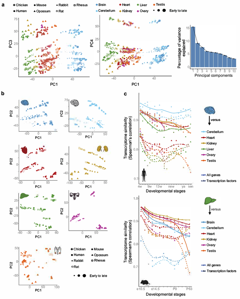
a, PC3 and PC4 of the PCA based on 7,696 1:1 orthologs depicted in Fig. 1b (each dot represents the median across replicates), and scree plot describing the amount of variance explained by the first 10 PCs. b, PCAs of individual organs (n = 7,696 1:1 orthologs). c, Correlation of expression levels throughout development between (top) human brain and the other organs (20,345 genes), (bottom) mouse liver and the other organs (21,798 genes). Similar patterns were observed using other organs as the focal organ, and species. For human, the prenatal data are in weeks (w) and postnatally ‘new’ means newborn, ‘sch’ school age (7-9 years), ‘ya’ young adult (25-32 years) and ‘sen’ senior (58-63 years).

Extended Data Figure 2 |. DDGs.

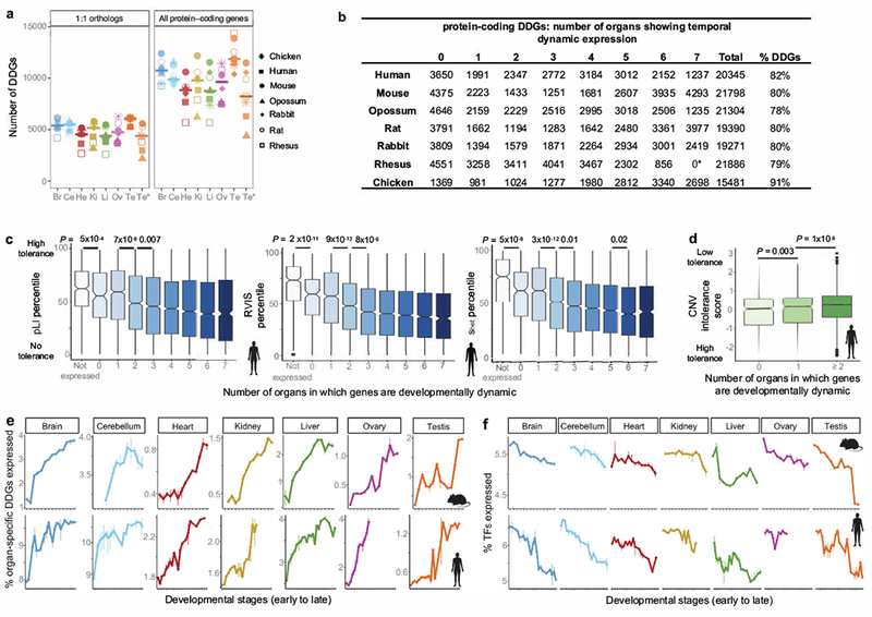
a, Number of DDGs identified in each organ and species using (left) the set of 7,696 1:1 orthologs and (right) the set of all protein-coding genes in each species. The horizontal bar depicts the median. Br: Brain, Cr: Cerebellum, He: Heart, Ki: Kidney, Li: Liver, Ov: Ovary, Te: Testis, Te*: Testis pre-sexual maturity. b, Number of DDGs per species, including number of organs where they show dynamic expression. *In rhesus ovary development is not covered, hence there are only 6 organs in total. c, Relationship between the number of organs in which genes show dynamic expression and the tolerance to functional variants as measured by: the probability of being loss-of-function intolerant (pLI score), the residual variation intolerance score (RVIS) and selection against heterozygous loss-of-function (s_het score) (n = 13,160 genes; Wilcoxon rank sum test, two-sided). d, Relationship between the number of organs in which genes show dynamic expression and intolerance to duplication and deletion variants (CNV intolerance score; n = 15,728 genes; Wilcoxon rank sum test, two-sided). e, Percentage of organ-specific expressed DDGs at each developmental stage. Bars indicate the range between the replicates. For the brain tissues, DDGs are organ-specific in brain and/or cerebellum. Time-points on the x-axis described in Fig. 1a. f, Percentage of TFs expressed at each developmental stage. Bars indicate the range between the replicates. Time-points on the x-axis described in Fig. 1a. In c-d, box plots depict median ± 25th and 75th percentiles, whiskers at 1.5 times the interquartile range.

Extended Data Figure 3 |. Developmental correspondences across species.

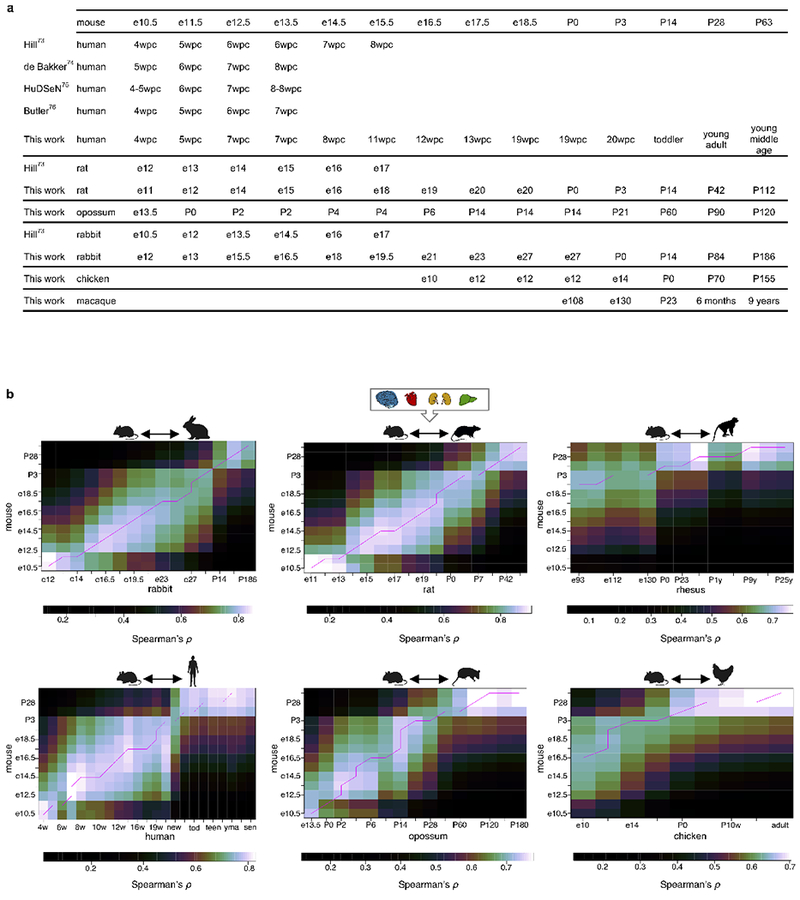
a, Developmental stage correspondences established in this study and correspondences based on the Carnegie staging (when available). b, Using mouse as a reference, a dynamic time warping algorithm was used to select the best alignment (pink line) between the time series based on stage transcriptome correlations combining all somatic organs (n = 8,940 genes/organ combinations). In the human correspondence, “new” means newborn, “tod” toddler (2-4 years), “teen” teenager (13-19 years), “yma” young middle age (39-41 years), “sen” senior (58-63 years).

Extended Data Figure 4 |. Periods of greater transcriptional change in mouse.

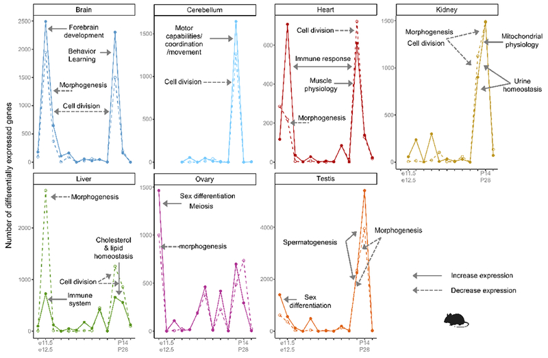
Number of genes differentially expressed between adjacent stages in each organ (log₂ fold change ≥ 0.5). Solid lines refer to genes that increase in expression and dashed lines to genes that decrease. The biological processes and phenotypes enriched at the peaks of differential expression are detailed in Supplementary Table 13.

Extended Data Figure 5 |. Periods of greater transcriptional change across species.

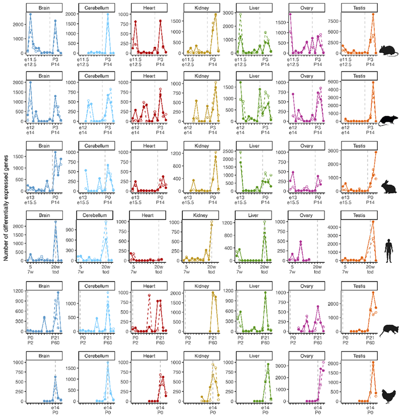
Number of genes differentially expressed between adjacent, species-matched, stages for each organ (log₂ fold change ≥ 0.5). Solid lines refer to genes that increase in expression and dashed lines to genes that decrease. The vertical dotted line marks birth.

Extended Data Figure 6 |. Organ-specific stage correspondences.

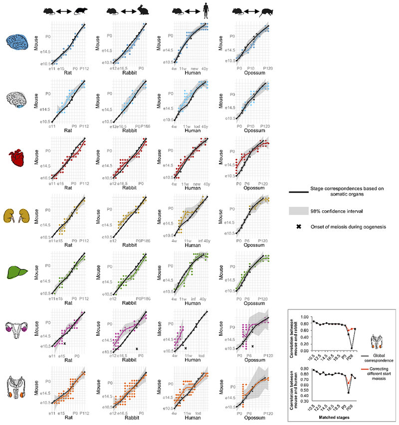
Comparison of the global stage correspondences (based on the combined expression of somatic organs; n = 8,940 genes/organ combinations; black line) with organ-specific correspondences (based on 2,727 genes for brain, 2,146 for cerebellum, 1,276 for heart, 1,486 for kidney, 1,305 for liver, 1,298 for ovary, and 2,153 for testis; colored lines). With the exception of early heart development in opossum and early ovary development in rabbit and human, the global correspondences are within the 98% confidence interval for predictions computed by the loess function (local polynomial regression) for each of the organ-specific correspondences (shaded grey area). The same applies to all organs in mouse-chicken and mouse-rhesus comparisons (data not shown). The inset on the bottom right, shows the Spearman correlation between mouse and rabbit (top) and mouse and human (bottom) for testis transcriptomes using the global stage correspondences (black line) or adjusting for the different start of meiosis across species (orange line; i.e. matching a P14 mouse with a young teenager in human and a P84 rabbit).

Extended Data Figure 7 |. Heterochronies in gonadal development.

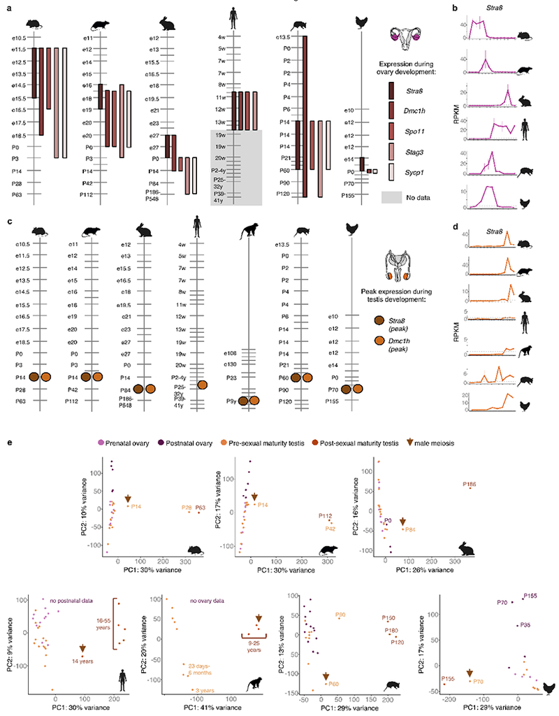
a, Temporal dynamics of meiotic genes during ovary development. SYCP1 is not expressed in human ovary. The genes SPO11 and STAG3 are not present in the chicken gene annotations used in this work. b, Expression of Stra8 during ovary development. The vertical bars show the range between the replicates and the horizontal dashed line marks 1 RPKM. c, Temporal dynamics of meiotic genes during testis development. The profiles of Stra8 and Dmc1 are represented not by their range of expression but by their highest peak of expression. In rhesus, meiosis is known to start around 3-4 years³⁶; our data suggest it had not yet started in the 3-year-old individuals examined. STRA8 is lowly expressed in the human testis. d, Expression of Stra8 during testis development. The vertical bars show the range between the replicates and the horizontal dashed line marks 1 RPKM. e, PCA of ovary and testis development for each species (n = 21,798 protein-coding genes in mouse, 19,390 in rat, 19,271 in rabbit, 20,345 in human, 21,886 in rhesus and 15,481 in chicken).

Extended Data Figure 8 |. Relationships between evolution and development.

a, Observed relationship between evolution and development. Divergence (horizontal distance) can be morphological or molecular. b, Transcriptome similarity between three species-pairs throughout development (matched stages) using 11,439 1:1 orthologs. Similar trends were obtained using all species-pairs. The weighted average Spearman correlation coefficients are −0.81 (P = 1 × 10⁻¹²) for the mouse-rat comparison, −0.69 (P = 2 × 10⁻¹¹) for mouse-human and −0.42 (P = 0.0004) for mouse-opossum. At the bottom are the Spearman correlations between transcriptome correlation coefficients and matched developmental time for each organ and species-pair (**P < 0.02, *P < 0.05). Lines were estimated through linear regression and the 95% confidence interval is shown in grey. c, Tolerance to loss-of-function variants (pLI score) for genes with different developmental trajectories in human (top) and mouse (bottom). Lower values mean less tolerance. The pLI scores used for mouse genes are from their human orthologs. The P-values refer to early vs. late comparisons, Wilcoxon rank sum test, two-sided. Box plots depict the median ± 25th and 75th percentiles, whiskers at 1.5 times the interquartile range. d, Percentage of lethal and subviable genes expressed throughout development among a set of 2,686 neutrally ascertained mouse knockouts (top) and the same after excluding housekeeping genes (bottom). Spearman correlations at the bottom of each plot. Lines were estimated through linear regression and the 95% confidence interval is shown in grey.

Extended Data Figure 9 |. Pleiotropy as a determinant of the evolution of development.

a, Relationship between tissue- and time-specificity. Gene developmental profiles illustrate the extremes of the indexes, which range from 0 (broad time/spatial expression) to 1 (specific time/spatial expression). In the gene plots, the x-axis shows the samples ordered by stage and organ and the y-axis shows expression levels. b, Functional constraints (measured by pLI) decrease with increasing time- and tissue-specificity (n = 9,965 genes). **All P < 0.01, Wilcoxon rank sum test, two-sided. c, Tissue- and time-specificity of mouse genes identified as lethal, subviable, or viable (n = 2,686; Wilcoxon rank sum test, two-sided). d, Levels of functional constraint as measured by RVIS, s_het, and pLI scores for the human orthologs of genes identified as lethal, subviable and viable in mouse (n = 2,408; Wilcoxon rank sum test, two-sided). e, Tissue- and time-specificity of genes with different developmental trajectories in human (top) and the same after excluding housekeeping genes (bottom). The P-values refer to early vs. late comparisons, Wilcoxon rank sum test, two-sided. In b-e, the box plots depict the median ± 25th and 75th percentiles, whiskers at 1.5 times the interquartile range.

Extended Data Figure 10 |. Evolution of developmental trajectories.

a, Number of genes in each organ that evolved new trajectories across the phylogeny. Includes genes that differ between opossum and eutherians, for which the change cannot be polarized because of the lack of an outgroup. b, Distribution of trajectory changes among organs for the different species. The number of genes that changed in each organ is depicted in Fig. 4b. Humans show a relative excess of changes in brain tissues and a relative paucity in testis. **P = 2 × 10⁻⁵ for brain, P = 0.02 for cerebellum and P = 1 × 10⁻¹⁰ for testis (from binomial tests where the probability of success is derived from what is observed in mouse, rat and rabbit). c, Genes tested for trajectory changes (7,020 genes) in mouse (top) and human (bottom) have significantly lower tissue- and time-specificity than genes not tested for trajectory changes (13,325 genes in mouse and 14,778 in human, Wilcox rank sum test, two-sided). d, Genes with trajectory changes in mouse (top) and human (bottom) have similar or lower tissue- and time-specificity than genes with conserved trajectories (Wilcox rank sum test, two-sided, ‘N.S.’ means non-significant). e, Number of organs in which genes evolved new trajectories in the different species. In c-d, the box plots depict the median ± 25th and 75th percentiles, whiskers at 1.5 times the interquartile range.

References

- 1.Pantalacci S & Semon M Transcriptomics of Developing Embryos and Organs: A Raising Tool for Evo-Devo. J. Exp. Zool. 00B, 1–9 (2014). [DOI] [PubMed] [Google Scholar]
- 2.Silbereis JC, Pochareddy S, Zhu Y, Li M & Sestan N The Cellular and Molecular Landscapes of the Developing Human Central Nervous System. Neuron 89, 248–268 (2016). [DOI] [PMC free article] [PubMed] [Google Scholar]
- 3.DeFalco T & Capel B Gonad morphogenesis in vertebrates: divergent means to a convergent end. Annu. Rev. Cell. Dev. Biol. 25, 457–482 (2009). [DOI] [PMC free article] [PubMed] [Google Scholar]
- 4.Abzhanov A von Baer’s law for the ages: lost and found principles of developmental evolution. Trends Genet. 29, 712–722 (2013). [DOI] [PubMed] [Google Scholar]
- 5.Kalinka AT & Tomancak P The evolution of early animal embryos: conservation or divergence? Trends Ecol. Evol. 27, 385–393 (2012). [DOI] [PubMed] [Google Scholar]
- 6.Ferner K, Schultz JA & Zeller U Comparative anatomy of neonates of the three major mammalian groups (monotremes, marsupials, placentals) and implications for the ancestral mammalian neonate morphotype. J. Anat. 231, 798–822 (2017). [DOI] [PMC free article] [PubMed] [Google Scholar]
- 7.Dickinson ME et al. High-throughput discovery of novel developmental phenotypes. Nature 537, 508–514 (2016). [DOI] [PMC free article] [PubMed] [Google Scholar]
- 8.Petrovski S, Wang Q, Heinzen EL, Allen AS & Goldstein DB Genic intolerance to functional variation and the interpretation of personal genomes. PLoS Genet. 9, e1003709 (2013). [DOI] [PMC free article] [PubMed] [Google Scholar]
- 9.Lek M et al. Analysis of protein-coding genetic variation in 60,706 humans. Nature 536, 285–91 (2016). [DOI] [PMC free article] [PubMed] [Google Scholar]
- 10.Cassa CA et al. Estimating the selective effects of heterozygous protein-truncating variants from human exome data. Nat. Genet. 49, 806–810 (2017). [DOI] [PMC free article] [PubMed] [Google Scholar]
- 11.Ruderfer DM et al. Patterns of genic intolerance of rare copy number variation in 59,898 human exomes. Nat. Genet. 48, 1107–1111 (2016). [DOI] [PMC free article] [PubMed] [Google Scholar]
- 12.Hill MA Embryology Carnegie Stage Comparison. https://jeltsch.org/carnegie_stage_comparison (2017). [Google Scholar]
- 13.de Bakker BS et al. An interactive three-dimensional digital atlas and quantitative database of human development. Science 354 (2016). [DOI] [PubMed] [Google Scholar]
- 14.Kerwin J et al. The HUDSEN Atlas: a three-dimensional (3D) spatial framework for studying gene expression in the developing human brain. J. Anat. 217, 289–299 (2010). [DOI] [PMC free article] [PubMed] [Google Scholar]
- 15.Butler H & Juurlink BHJ An Atlas for Staging Mammalian and Chick Embryos. (CRC Press, Boca Raton, Fla., 1987). [Google Scholar]
- 16.Smith KK Early development of the neural plate, neural crest and facial region of marsupials. J. Anat. 199, 121–131 (2001). [DOI] [PMC free article] [PubMed] [Google Scholar]
- 17.Dillman AA et al. mRNA expression, splicing and editing in the embryonic and adult mouse cerebral cortex. Nat. Neurosci. 16, 499–506 (2013). [DOI] [PMC free article] [PubMed] [Google Scholar]
- 18.Glucksmann A Sexual dimorphism in mammals. Biol. Rev. 49, 423–475 (1974). [DOI] [PubMed] [Google Scholar]
- 19.Feng CW, Bowles J & Koopman P Control of mammalian germ cell entry into meiosis. Mol. Cell. Endocrinol. 382, 488–497 (2014). [DOI] [PubMed] [Google Scholar]
- 20.Soumillon M et al. Cellular source and mechanisms of high transcriptome complexity in the mammalian testis. Cell Rep. 3, 2179–2190 (2013). [DOI] [PubMed] [Google Scholar]
- 21.Ungewitter EK & Yao HH How to make a gonad: cellular mechanisms governing formation of the testes and ovaries. Sex. Dev. 7, 7–20 (2013). [DOI] [PMC free article] [PubMed] [Google Scholar]
- 22.Roux J & Robinson-Rechavi M Developmental Constraints on Vertebrate Genome Evolution. PLoS Genet. 4, 10 (2008). [DOI] [PMC free article] [PubMed] [Google Scholar]
- 23.Kalinka AT et al. Gene expression divergence recapitulates the developmental hourglass model. Nature 468, 811–814 (2010). [DOI] [PubMed] [Google Scholar]
- 24.Hu H et al. Constrained vertebrate evolution by pleiotropic genes. Nat. Ecol. Evol. 1, 1722–1730 (2017). [DOI] [PubMed] [Google Scholar]
- 25.Hazkani-Covo E, Wool D & Graur D In search of the vertebrate phylotypic stage: a molecular examination of the developmental hourglass model and von Baer’s third law. J. Exp. Zool. B. Mol. Dev. Evol. 304, 150–8 (2005). [DOI] [PubMed] [Google Scholar]
- 26.Garfield DA & Wray GA Comparative embryology without a microscope: using genomic approaches to understand the evolution of development. J. Biol. 8, 65 (2009). [DOI] [PMC free article] [PubMed] [Google Scholar]
- 27.Koscielny G et al. The International Mouse Phenotyping Consortium Web Portal, a unified point of access for knockout mice and related phenotyping data. Nucleic Acids Res. 42, D802–9 (2014). [DOI] [PMC free article] [PubMed] [Google Scholar]
- 28.Kosiol C et al. Patterns of Positive Selection in Six Mammalian Genomes. PLoS Genet. 4, e1000144 (2008). [DOI] [PMC free article] [PubMed] [Google Scholar]
- 29.Kaessmann H Origins, evolution, and phenotypic impact of new genes. Genome Res. 20, 1313–1326 (2010). [DOI] [PMC free article] [PubMed] [Google Scholar]
- 30.Stern DL Evolutionary developmental biology and the problem of variation. Evolution 54, 1079–91 (2000). [DOI] [PubMed] [Google Scholar]
- 31.Carroll SB Evolution at two levels: on genes and form. PLoS Biol 3, e245 (2005). [DOI] [PMC free article] [PubMed] [Google Scholar]
- 32.Duret L & Mouchiroud D Determinants of substitution rates in mammalian genes: expression pattern affects selection intensity but not mutation rate. Mol. Biol. Evol. 17, 68–74 (2000). [DOI] [PubMed] [Google Scholar]
- 33.Winter E, Goodstadt L & Ponting CP Elevated Rates of Protein Secretion, Evolution, and Disease Among Tissue-Specific Genes. Genome Res. 14, 54–61 (2004). [DOI] [PMC free article] [PubMed] [Google Scholar]
- 34.Galis F & Metz J Testing the Vulnerability of the Phylotypic Stage: On Modularity and Evolutionary Conservation. Journal of Experimental Zoology (Mol Dev Evol) 291, 195–204 (2001). [DOI] [PubMed] [Google Scholar]
- 35.Sears K, Maier JA, Sadier A, Sorensen D & Urban DJ Timing the developmental origins of mammalian limb diversity. Genesis 56 (2018). [DOI] [PubMed] [Google Scholar]
- 36.Plant TM, Ramaswamy S, Simorangkir D & Marshall GR Postnatal and pubertal development of the rhesus monkey (Macaca mulatta) testis. Ann. N. Y. Acad. Sci. 1061, 149–162 (2005). [DOI] [PubMed] [Google Scholar]
Methods references
- 37.Bruneau BG Signaling and transcriptional networks in heart development and regeneration. Cold Spring Harb. Perspect. Biol. 5, a008292 (2013). [DOI] [PMC free article] [PubMed] [Google Scholar]
- 38.Carelli FN, Liechti A, Halbert J, Warnefors M & Kaessmann H Repurposing of promoters and enhancers during mammalian evolution. Nat. Commun. 9, 4066 (2018). [DOI] [PMC free article] [PubMed] [Google Scholar]
- 39.Marin R et al. Convergent origination of a Drosophila-like dosage compensation mechanism in a reptile lineage. Genome Res. 27, 1974–1987 (2017). [DOI] [PMC free article] [PubMed] [Google Scholar]
- 40.Wu TD & Nacu S Fast and SNP-tolerant detection of complex variants and splicing in short reads. Bioinformatics 26, 873–881 (2010). [DOI] [PMC free article] [PubMed] [Google Scholar]
- 41.Anders S, Pyl PT & Huber W HTSeq--a Python framework to work with high-throughput sequencing data. Bioinformatics 31, 166–169 (2015). [DOI] [PMC free article] [PubMed] [Google Scholar]
- 42.Robinson MD, McCarthy DJ & Smyth GK edgeR: a Bioconductor package for differential expression analysis of digital gene expression data. Bioinformatics 26, 139–140 (2010). [DOI] [PMC free article] [PubMed] [Google Scholar]
- 43.Li H et al. The Sequence Alignment/Map format and SAMtools. Bioinformatics 25, 2078–2079 (2009). [DOI] [PMC free article] [PubMed] [Google Scholar]
- 44.Picard. http://broadinstitute.github.io/picard (2015)
- 45.Le S, Josse J & Husson F FactoMineR: An R Package for Multivariate Analysis. J. Stat. Softw. 25 (2008). [Google Scholar]
- 46.Core Team R. R: A Language and Environment for Statistical Computing. (2014). [Google Scholar]
- 47.Anavy L et al. BLIND ordering of large-scale transcriptomic developmental timecourses. Development 141, 1161–6 (2014). [DOI] [PubMed] [Google Scholar]
- 48.Love MI, Huber W & Anders S Moderated estimation of fold change and dispersion for RNA-seq data with DESeq2. Genome Biol. 15, 550 (2014). [DOI] [PMC free article] [PubMed] [Google Scholar]
- 49.Quinlan AR & Hall IM BEDTools: a flexible suite of utilities for comparing genomic features. Bioinformatics 26, 841–842 (2010). [DOI] [PMC free article] [PubMed] [Google Scholar]
- 50.Nueda MJ, Tarazona S & Conesa A Next maSigPro: updating maSigPro bioconductor package for RNA-seq time series. Bioinformatics 30, 2598–2602 (2014). [DOI] [PMC free article] [PubMed] [Google Scholar]
- 51.Conesa A, Nueda MJ, Ferrer A & Talon M maSigPro: a method to identify significantly differential expression profiles in time-course microarray experiments. Bioinformatics 22, 1096–1102 (2006). [DOI] [PubMed] [Google Scholar]
- 52.Zhang HM et al. AnimalTFDB 2.0: a resource for expression, prediction and functional study of animal transcription factors. Nucleic Acids Res. 43, D76–81 (2015). [DOI] [PMC free article] [PubMed] [Google Scholar]
- 53.Giorgino T Computing and Visualizing Dynamic Time Warping Alignments in R: The dtw Package. J. Stat. Softw. 31, 1–24 (2009). [Google Scholar]
- 54.Clancy B, Darlington RB & Finlay BL Translating developmental time across mammalian species. Neuroscience 105, 7–17 (2001). [DOI] [PubMed] [Google Scholar]
- 55.Smith KK Craniofacial development in marsupial mammals: developmental origins of evolutionary change. Dev. Dyn. 235, 1181–1193 (2006). [DOI] [PubMed] [Google Scholar]
- 56.Futschik ME & Carlisle B Noise-robust soft clustering of gene expression time-course data. J. Bioinform. Computat. Biol. 3, 965–988 (2005). [DOI] [PubMed] [Google Scholar]
- 57.Kumar L & Futschik M Mfuzz: A software package for soft clustering of microarray data. Bioinformation 2, 5–7 (2007). [DOI] [PMC free article] [PubMed] [Google Scholar]
- 58.Eisenberg E & Levanon EY Human housekeeping genes, revisited. Trends Genet. 29, 569–574 (2013). [DOI] [PubMed] [Google Scholar]
- 59.Domazet-Loso T & Tautz D A phylogenetically based transcriptome age index mirrors ontogenetic divergence patterns. Nature 468, 815–818 (2010). [DOI] [PubMed] [Google Scholar]
- 60.Zhang YE, Vibranovski MD, Landback P, Marais GA & Long M Chromosomal redistribution of male-biased genes in mammalian evolution with two bursts of gene gain on the X chromosome. PLoS Biol. 8, e1000494 (2010). [DOI] [PMC free article] [PubMed] [Google Scholar]
- 61.Yanai I et al. Genome-wide midrange transcription profiles reveal expression level relationships in human tissue specification. Bioinformatics 21, 650–9 (2005). [DOI] [PubMed] [Google Scholar]
- 62.Hensman J, Lawrence ND & Rattray M Hierarchical Bayesian modelling of gene expression time series across irregularly sampled replicates and clusters. BMC Bioinformatics 14, 252 (2013). [DOI] [PMC free article] [PubMed] [Google Scholar]
- 63.Hensman J, Rattray M & Lawrence ND Fast Nonparametric Clustering of Structured Time-Series. IEEE Trans. Pattern. Anal. Mach. Intell. 37, 383–393 (2015). [DOI] [PubMed] [Google Scholar]
- 64.Hensman J, Rattray M & Lawrence ND Fast Variational Inference in the Conjugate Exponential Family. Pattern Analysis and Machine Intelligence, IEEE Transactions on (2014). [Google Scholar]
- 65.Kumar S, Stecher G, Suleski M & Hedges SB TimeTree: A Resource for Timelines, Timetrees, and Divergence Times. Mol. Biol. Evol. 34, 1812–1819 (2017). [DOI] [PubMed] [Google Scholar]
- 66.Vickaryous MK & Hall BK Human cell type diversity, evolution, development, and classification with special reference to cells derived from the neural crest. Biol. Rev. Camb. Philos. Soc. 81, 425–455 (2006). [DOI] [PubMed] [Google Scholar]
- 67.Wickham H ggplot2: Elegant Graphics for Data Analysis. (Springer-Verlag New York, 2009). [Google Scholar]
- 68.Auguie B gridExtra: Miscellaneous Functions for “Grid” Graphics. (2015). [Google Scholar]
- 69.Wickham H Reshaping Data with the reshape Package. J. Stat. Softw. 21 (2007). [Google Scholar]
- 70.Wickham H The Split-Apply-Combine Strategy for Data Analysis. J. Stat. Softw. 40 (2011). [Google Scholar]
- 71.Kassambara A & Mundt F factoextra: Extract and Visualize the Results of Multivariate Data Analyses. (2017). [Google Scholar]
- 72.Wang J, Vasaikar S, Shi Z, Greer M & Zhang B WebGestalt 2017: a more comprehensive, powerful, flexible and interactive gene set enrichment analysis toolkit. Nucleic Acids Res 45, W130–37 (2017). [DOI] [PMC free article] [PubMed] [Google Scholar]
Associated Data
This section collects any data citations, data availability statements, or supplementary materials included in this article.