Multiconfigurational Coarse-Grained Molecular Dynamics

Abstract

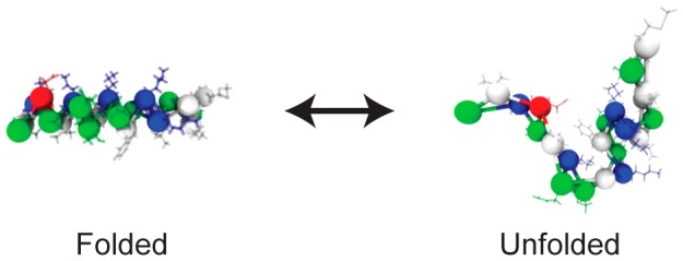
Standard low resolution coarse-grained modeling techniques have difficulty capturing multiple configurations of protein systems. Here, we present a method for creating accurate coarse-grained (CG) models with multiple configurations using a linear combination of functions or “states”. Individual CG models are created to capture the individual states, and the approximate coupling between the two states is determined from an all-atom potential of mean force. We show that the resulting multiconfiguration coarse-graining (MCCG) method accurately captures the transition state as well as the free energy between the two states. We have tested this method on the folding of dodecaalanine, as well as the amphipathic helix of endophilin.

Introduction

Biomolecular systems are inherently multiscale, involving the interplay of many length and time scales working in concert. As a result, the theoretical methods used to understand these systems must be able to take into account this multiscale nature. Although molecular dynamics (MD) simulations can be used to successfully probe biomolecular processes and interactions in ways that can complement experimental results,¹ standard MD methods are limited to length and time scales that may be unable to accurately characterize many biomolecular phenomena. These systems require the use of multiscale MD methods,²⁻⁴ where low resolution, or coarse-grained (CG), models of biological molecules are developed to reduce the computational cost of such simulations, all while attempting to maintain the fundamental physics and chemistry underlying the biomolecular processes.^4,5 The use of low-resolution CG models can be used to probe important processes such as protein–protein interactions,⁶⁻⁸ membrane remodeling by proteins,⁹⁻¹⁶ and large-scale protein conformational changes.¹⁷

Current CG models are often unable to accurately reproduce large conformational changes in proteins^2,3 and are thus typically best suited to model a single protein conformation. However, even CG models that may be able to capture multiple protein conformations are still unable to reproduce the free energy difference between the two states and the transition barrier.^18,19 This has been seen for CG models that were parametrized with a top-down approach, incorporating information from experiment, or a bottom-up approach, where high frequency motions in higher resolution all-atom (AA) simulations are integrated out to generate smoother, but less detailed interaction potentials. The popular MARTINI protein force field,^20,21 a top-down CG model, requires an elastic network on the peptide backbone to maintain secondary structure and is therefore restrained to the native state.^3,22 Top-down models, including OPEP²³ and MARTINI, in general are not guaranteed to generate the correct kinetics or sample the correct distribution of states. Bottom-up CG approaches, including relative entropy minimization²⁴ (REM) and multiscale coarse-graining²⁵⁻²⁷ (MS-CG), can at best capture portions of multiple conformations but less accurately capture the free energy difference between the states and the transition barrier.²⁸⁻³⁰ This limitation of MS-CG and REM is not inherent to the methods themselves but instead to the practical considerations when building the models, including limiting the models to pair interactions and not having unique interactions between all CG sites. This deficiency of current CG modeling techniques impedes the study of complex, multiscale biophysical phenomena, including, for example, actin polymerization, where the ATP hydrolysis within actin as well as actin conformational change drive polymerization and depolymerization,³¹ or molecular motors such as myosin where ATP hydrolysis and other effects drive large scale conformational change.

Much of the previous work on multiconfiguration CG modeling has been focused on developing fine-grained, Cα elastic network models (ENMs) of proteins that can switch between two or more equilibrium states.³²⁻³⁶ These methods treat the individual equilibrium configurations as discrete states and use a two-state-like mixing approach to couple the discrete states while also providing the smooth saddle point between the states. The benefit of such an approach is that the CG model can sample configurations, or states, corresponding to very different protein structures, but switching between structures in these simulations is not parametrized in a multiscale manner that accurately reproduces key features in the potential of mean force (PMF) for the conformational transition, such as the transition barrier and the free energy difference between the conformational states. A recent study by Bereau and Rudzinski³⁷ similarly separates the system into distinct conformational basins and uses a surface hopping-like scheme to switch between the states describing those basins. However, constraints need to be placed on the system to reproduce the correct probability distribution of states and the algorithm also does not conserve energy on an overall continuous CG potential.

In this work, we introduce a new multiconfiguration coarse-graining (MCCG) method that can both switch between CG models that describe different parts of the molecular conformational during the course of a MD simulation and directly take into account key features of the AA PMF to couple the individual CG models. (Hence the term “multiconfigurational” is used for the method.) This multiscale approach results in CG simulations that can reproduce the transition barrier and the free energy difference between the states of the AA PMF but with much fewer degrees of freedom than the AA simulation. In the MCCG method presented here, a two-state mixing approach is used, where the diagonal elements of a two state Hamiltonian-like matrix represent the free energy surface for each of the independently developed CG models. MCCG thus at the outset takes advantage of the strength of CG models to accurately reproduce protein conformations in individual free energy basins. Each of these states can represent the system in a different basin, e.g., folded or unfolded, open or closed, in membrane or in solution. Importantly, off-diagonal elements in the 2 × 2 quantum-like matrix represent the thermodynamic coupling between the CG states. However, that coupling is assumed to be only a function of a few key CG collective variables (CVs) that can well describe the transition between states. In turn, this coupling can be directly calculated from the AA PMF in a way that incorporates the differences between the CG potential energy surfaces and the full AA PMF. The MCCG methodology thus results in a multiconfigurational CG simulation on a continuous CG free energy surface that can reproduce the features of the AA PMF, including the saddle point barrier, in terms of CG CVs that describe the transition between the CG structural states. The resulting model can also reasonably reproduce PMFs along other CVs that were not a part of the original model development, with some caveats.

Theory and Methods

Theory

We demonstrate here a method to build CG models that can accurately reproduce an AA PMF for conformational change. Our strategy is as follows: a combined effective free energy surface in the CG variables is defined using a two-state Hamiltonian-like matrix, whose state elements encompass two different configurations of a protein, as well as a coupling term between those two states. The combined energy surface is then obtained by diagonalizing this Hamiltonian, and the coupling term between the two configurations is next defined in terms of a projection on one or more collective variables of the AA PMF.

To develop such CG models that can describe multiple conformational basins and transitions between them in terms of the many-dimensional CG coordinates R^N, we first treat the individual structures as discrete “states” with separate CG force fields and hence diabatic-like energy surfaces, labeled V₁₁(R^N) and V₂₂(R^N). Here, we are limiting ourselves to the case where only two CG structural models (states) are considered, but in principle, more than two can be treated (albeit with added complication). Although our system is not a quantum mechanical system (it is purely a linear combination of CG energy surfaces), treating the individual CG structures as discrete thermodynamic states within an effective quantum-like two-state coupling picture allows us to conveniently describe the system using a 2 × 2 matrix Hamiltonian, as in the case of electron transfer³⁸

1

where V₁₁(R^N) and V₂₂(R^N) are the CG energy surfaces of the discrete (diabatic) thermodynamic CG states, and V₁₂(R^N) is a coupling between the two CG states. In the MCCG model, the V₁₁(R^N) and V₂₂(R^N) terms are determined by the CG effective force fields describing the individual “states”, i.e., particular conformational basin regions in the overall energy landscape of the CG variables. By using the following characteristic equation, the CG energy surface, E, can be created that includes a smooth saddle point between the free energy surfaces of the individual CG models:

2

We note that this approach is similar in spirit to the Empirical Valence Bond (EVB) approach³⁹ but that these present equations are defined at the CG, rather than AA, level as in EVB.

If there is a nontrivial solution to the characteristic equation above, then the secular equation can be solved for the lowest energy eigenvalue for every value of the CG coordinate R^N:

3

resulting in the following standard 2 × 2 quantum-like expression for the coupled energy surface in the CG variables:

4

We note that previously developed multistate CG ENM methods have either treated the off-diagonal coupling term, V₁₂(R^N), as a constant^32,33,36 or have used a second-order expansion around the saddle point to approximate the coupling.^34,40

A key goal in this work is to develop a method for determining V₁₂(R^N) using information obtained from AA simulations, which allows the CG system to reproduce one or more AA PMFs in certain collective variables (CVs) related to the conformational transition. To this end, we can first solve the solution in eq 3 for the off-diagonal coupling term, V₁₂(R^N), in terms of both the individual states and the total coupled potential energy surface:

5

Again, we stress that we are simply using a linear combination function to describe the overall coarse-grained (CG) system much like a two-state Hamiltonian matrix in the theory of electron transfer or the empirical valence bond method. Therefore, the lowest eigenvalue of eq 1E(R^N) should be thought of as the “correct” overall energy surface for the CG variables that includes the proper transitions between conformations. Given this, eq 3 should then be considered as the definition of V₁₂(R^N).

It must be stressed here that the most general form of the coupling element above, V₁₂(R^N), is exceptionally difficult to know. In a bottom-up CG model, if one has perfect sampling as well as a complete physically accurate basis set to represent the CG interactions, then one will simply have E(R^N) and there is no need for the MCCG approach at all. However, this is rarely if ever going to be the case. It is more likely the case that any CG approach (bottom-up or top-down or something in-between) will provide reasonable models for the conformational basins in the CG energy landscape, and one may even obtain these models by using different CG methodologies in each basin. As such, in order to then derive an approximate expression for V₁₂(R^N) in which we can more easily calculate the relevant terms, we make two assumptions. First, we make the assumption that the CG energy function in the CG variables can approximate the true many-body AA PMF projected onto the CG variables. Here, we will thus treat the AA PMF projected onto the CG variables as the “true” system PMF, but we note that this function may also be estimated using force-pulling experiments or constructed “top-down” in some ad hoc (or other) manner of modeling. In other words, it should not be misunderstood here that only an AA PMF can be used in the approach about to be presented. Second, and most importantly, we assume that we can describe the process of transitioning from energy basin V₁₁(R^N) to V₂₂(R^N) with a single, or small collection of, collective variables (CVs) defined here as Q. These collective variables are a low dimensional projection defined from the full set of CG variables, R^N.

Therefore, with these key assumptions stated above in hand, the off-diagonal coupling can be rewritten in terms of the reduced dimensional PMFs of the CG diabatic states in terms of the CVs, defined as F₁₁(Q) and F₂₂(Q), as well as the AA PMF similarly projected onto the CVs, such that

6

For F_AA(Q), we also define that there is a function that maps the AA coordinates onto the CG CV, Q. Using only the collective variables also simplifies the calculation of the AA PMF, which can only be tractably calculated for a small collection of variables. By including the off-diagonal coupling between states in a way that is determined directly from the AA PMF, the free energy surface of the MCCG model can reproduce the AA PMF in terms of CG CVs.

We note that, if the components of the coupling term are calculated perfectly, the MCCG PMF will then match the AA PMF for the chosen CVs when the MCCG simulation is run for the full set of CG variables R^N. However, entropic and other contributions from the AA system may not have been fully accounted for in the CG potential energy terms nor in its projection along the CVs, Q. To account for this at least in part, V₁₂(Q) may be iteratively updated to achieve better agreement between the AA and CG PMFs along the CVs, Q. The coupling term V₁₂(Q) is iteratively updated to improve the resulting MCCG PMF by adding the difference between the fine-grained (e.g., AA) PMF F_AA(Q) and the MCCG PMF iteration F_MCCGⁱ(Q) to the coupling term:

7

where α is a tuning parameter to ensure convergence. Successive updates to the off-diagonal coupling term will then drive the MCCG PMF to approach the AA PMF along Q.

Simulation Details

AA Simulations

All-atom (AA) simulations were performed with the GROMACS (version 5) simulation suite⁴¹ using the CHARMM36 force field.⁴² Simulations were integrated with a 2 fs time step. Nonbonded van der Waals interactions were switched to zero between 1.0 and 1.2 nm. Electrostatic interactions were evaluated using Particle Mesh Ewald.⁴³ Bonds to hydrogen were constrained using the LINCS algorithm.⁴⁴ Temperature was maintained at 310 K using the stochastic velocity rescaling thermostat⁴⁵ with a coupling time constant of 0.1 ps. The pressure was maintained isotropically in constant pressure simulations using the Parrinello–Rahman barostat⁴⁶ at a pressure of 1.0 bar, a compressibility of 4.5 × 10^–5, and a coupling time constant of 2.0 ps. Coordinates were saved every 1 ps.

AA System Initialization and Equilibration

The endophilin amphipathic helix H0 (Sequence: MSVAGLKKQFHKATQKVSEKVG) and the capped alanine 12-mer were each initialized in a linear configuration using the Molefacture plugin in VMD.⁴⁷ H0 and dodecaalanine were solvated using VMD in a TIP3P water box with a side length of 6.0 and 4.8 nm, respectively, and ionized with 150 mM NaCl. The two peptides were then energy-minimized using the steepest descent algorithm to a maximum force of 1000 kJ mol^–1 nm^–1; the systems converged within 500 steps. The peptides were then equilibrated for 1 ns in the isothermal–isobaric ensemble (NPT).

AA Production Simulations

Dodecaalanine (ALA-AA) was simulated for 1 μs in the canonical ensemble (constant NVT) to adequately sample the folding/unfolding process. Free energy surfaces and CG models were obtained from the single, 1 μs simulation. H0 was simulated (H0-AA) using temperature replica-exchange molecular dynamics⁴⁸ (T-REMD) with 72 temperature windows exponentially distributed from 310 to 565 K. Each temperature replica was first equilibrated at the respective temperature for 100 ps. Each temperature replica was then simulated for 100 ns, with exchanges occurring every 100 steps. The average exchange probability across all replicas was 25%. Free energy surfaces and CG models were obtained from the lowest temperature replica.

CG Simulations

Coarse-grained (CG) simulations were carried out using the LAMMPS simulation package.⁴⁹ Simulations were integrated with a 5.0 fs time step. Temperature was maintained using the Langevin thermostat⁵⁰ with a damping coefficient of 500 fs. Coordinates were saved every 200 time steps. MCCG simulations were performed using a newly designed plugin for the LAMMPS simulation package (https://github.com/mocohen/USER-MCCG), which interfaces with the PLUMED2 plugin.⁵¹ MCCG simulation parameters were the same as the CG simulations.

CG Models

Dodecaalanine

Four solvent free CG models of dodecaalanine were constructed from the 1 μs AA simulation. Each alanine residue was represented by a single bead corresponding to the α carbon, for a total of 12 CG beads for the whole peptide. Two methods for creating CG models were used: heterogeneous elastic networks⁵² (HENM) and Boltzmann Inversion (BI). HENM models of polyalanine were created using the full trajectory (ALA-HENM) as well as for the folded configurations (ALA-HENM-F). HENM models were constructed using a cutoff of 1.5 nm. BI models of polyalanine were created using the full trajectory (ALA-BI) as well as for only the unfolded configurations (ALA-BI-U), configurations with a helicity (Q_hel) less than 0.2. Each bead in the BI model was treated equivalently; models were constructed with a single bond, angle, dihedral, and nonbonded interaction. Each CG model of dodecaalanine was simulated for 4 billion time steps to obtain the free energy surfaces.

H0

Two solvent free CG models of H0 were constructed from the lowest temperature replica of the AA T-REMD simulation. Each residue was represented by a single bead corresponding to the Cα carbon for a total of 22 CG beads for the whole peptide. An HENM model of H0 was constructed using only the folded configurations (H0-HENM-F). The HENM model was constructed using a cutoff of 1.5 nm. A BI model of H0 was created using only the unfolded configurations (H0-BI-U). Each bead in the BI model was treated equivalently; models were constructed with a single bonded, angular, dihedral, and nonbonded interaction. Each CG model of H0 was simulated for 4 billion time steps to obtain the free energy surfaces.

MCCG Models

MCCG models were constructed for dodecaalanine (ALA-MCCG) and H0 (H0-MCCG) using the folded HENM and unfolded BI CG models for the two states. For the iterative procedure, α was set to be 1.

Results and Discussion

In this section, we demonstrate the ability of a coupled two-state MCCG system to capture the folding and unfolding of two different peptides: an alanine 12-mer and endophilin H0.

Dodecaalanine

Dodecaalanine was chosen to test our MCCG model because it has been used in previous studies that attempted to capture the folding and unfolding process of peptides.^29,30 We first simulated dodecaalanine for 1 μs using AA MD. This fine-grained simulation sampled folded, partially folded, globular, and extended configurations. The free energy surface (Figure 1) along the helicity (Q_hel) and radius of gyration (R_g) CVs shows a large free energy minimum in the unfolded configuration (Q_hel < 0.2) as well as a few small free energy minima in the helical configurations (Q_hel > 0.8). These two CVs have been previously³⁰ used to characterize the different conformations explored by dodecaalanine.

Figure 1.

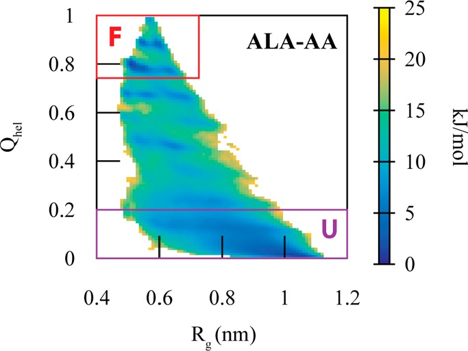
2D potential of mean force for the AA dodecaalanine (ALA-AA) system with mapped coordinates as a function of helicity (Q_hel) and radius of gyration (R_g). The folded state is denoted in the red square (F) and the unfolded state (U), in purple.

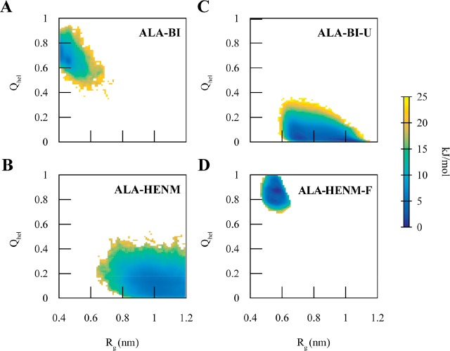
We chose a Cα mapping scheme, one CG site per residue at the Cα position, for each CG state model. A Cα CG mapping is able to characterize the difference between an unfolded and folded helix.⁵³ Using the Cα CG mapping, we developed two simple CG models to capture the folding and unfolding of the peptide using the AA trajectories. Both the Boltzmann Inversion (ALA-BI) and Heterogeneous Elastic Network (ALA-HENM) models developed from the AA trajectory of dodecaalanine failed to capture this transition, as seen in the 2D PMF (Figure 2). ALA-BI reproduces only portions of the folded configuration and is quite sticky; it stabilizes structures with small radius of gyration (R_g < 0.4), configurations that are not sampled in the AA simulation. ALA-HENM samples the unfolded configuration as well as a large number of high-energy states that are not sampled in the AA simulation. Previous studies by Carmichael and Shell,²⁹ as well as Rudzinski and Noid,³⁰ have also demonstrated the inability of more complicated CG methods to accurately capture both the folded and unfolded configurations of alanine polymers using the REM, iterative generalized Yvon-Born-Green,^54,55 and MS-CG techniques.

Figure 2.

2D potentials of the mean force of dodecalalanine as a function of helicity (Q_hel) and radius of gyration (R_g) for the four CG models: (A) Boltzmann inversion (ALA-BI); (B) heterogeneous elastic network model (ALA-HENM); Boltzmann inversion for the unfolded configurations (ALA-BI-U); (D) heterogeneous elastic network model for the folded configurations (ALA-HENM-F). ALA-BI and ALA-HENM both cannot reproduce the AA mapped PMF and do not sample portions of the AA mapped PMF well. ALA-BI-U reproduces the unfolded portion of the AA PMF, and ALA-HENM reproduces the folded portion of the AA PMF.

We next parametrized separate CG models to model the folded and unfolded configurations. A BI CG model parametrized solely from AA coordinates of the unfolded configuration (ALA-BI-U) reproduced the unfolded portion of the 2D PMF, and a heterogeneous Elastic Network CG model parametrized solely from AA coordinates of the folded configuration (ALA-HENM-F) reproduced the folded portion of the 2D PMF (Figure 2). While these simple CG models reproduce the general shape of the unfolded and folded areas of the PMF, they do not contain some of the local minima observed in the AA PMF. This is to be expected, as CG models generally smooth out the PMF. However, more features could be captured in the individual CG models for the folded and unfolded states if more sophisticated CG modeling techniques, such as MS-CG and REM, are used to build the diabatic states.

Using these CG models as the diabatic states and the AA and CG 2D PMFs to calculate the coupling, we constructed an MCCG model of dodecalanine (ALA-MCCG). The coupling term V₁₂(Q) was mostly localized to the transition region between the two states (Figure 3). Due to the large transition region, the coupling is required to operate over a reasonably large portion of conformational space. The resulting 2D PMF from the MCCG simulations of ALA-MCCG show sampling in both the folded and unfolded configurations, with transitions between the two states (Figure 3).

Figure 3.

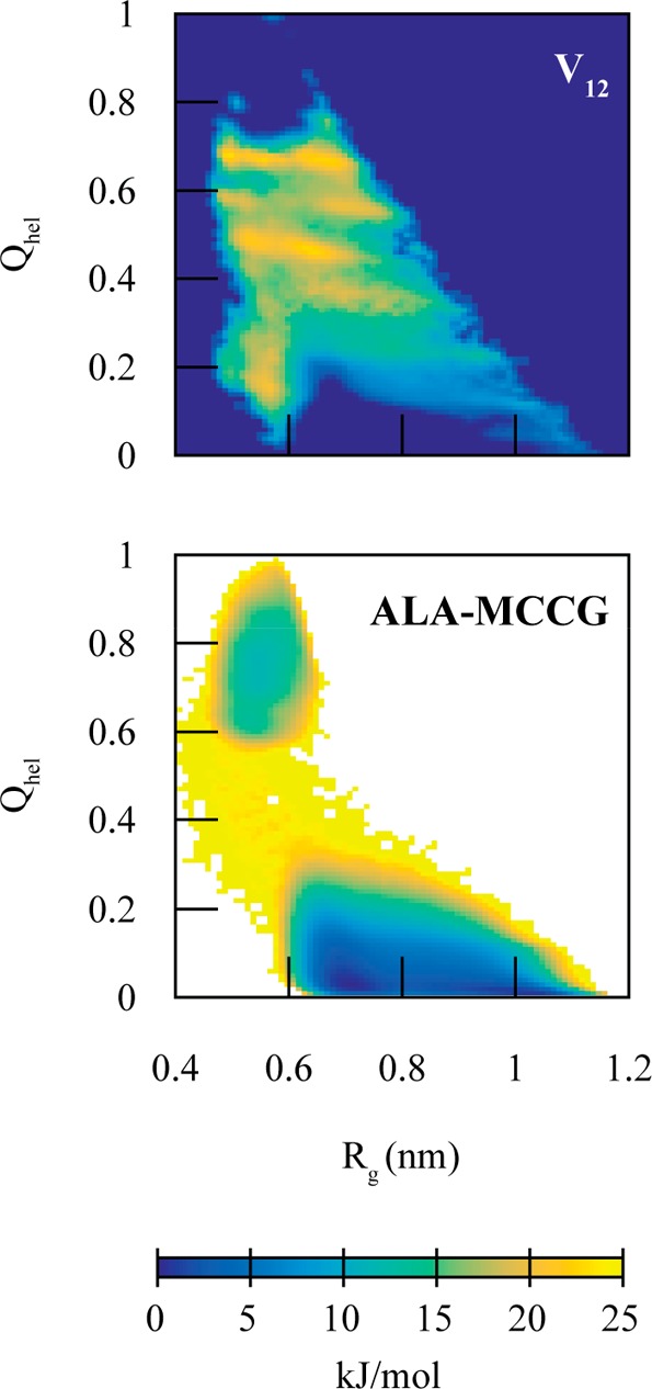
(Top) Tabulated coupling term (V₁₂(Q)), used for the dodecaalanine MCCG model, as a function of helicity (Q_hel) and radius of gyration (R_g). (Bottom) Resulting MCCG PMF for dodecaalanine (ALA-MCCG). ALA-MCCG reproduces two-state behavior but does not reproduce the barrier height or well depths.

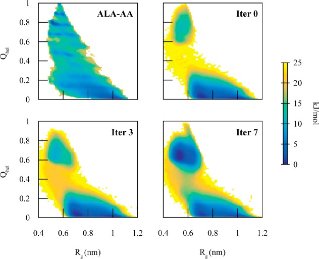
However, while the MCCG model was able to describe the two-state behavior of dodecaalanine, it was not able to accurately reproduce the barrier height nor the free energy difference between the two configurations. The high PMF barrier, 25 kJ/mol, in the MCCG model versus 15 kJ/mol in the AA model suggested that the coupling in the transition region is too low. We therefore refined the MCCG model by using the iterative procedure described in eq 7. Since the MCCG PMF and AA PMF are most different in the transition region, this slowly increases the coupling in the transition region, allowing the MCCG PMF barrier to reproduce the AA PMF barrier. As seen in Figure 4, the iterative MCCG procedure reduces the free energy barrier to 20 kJ/mol by the third iteration and 17 kJ/mol (within an order of k_bT) by the seventh iteration. Additionally, the PMF well depths, at 0 kJ/mol for both states in the AA PMF, are matched by the seventh iteration. It should again be noted that the AA PMF contains at least 10 local minima, which are smoothed out in the CG PMF. While MCCG substantially improves the transition region, it should not be expected to improve all other aspects of the CG model, especially features in the diabatic wells. The primary motions of the system are driven by the diabatic potentials; it is only in the transition region that the coupling term has its largest effect. Nevertheless, even with the diabatic states derived from simple CG models, MCCG can more accurately reproduce the overall AA PMF along the chosen CVs compared to more sophisticated (and as of yet unknown) CG modeling techniques.

Figure 4.

2D PMFs as a function of helicity (Q_hel) and radius of gyration (R_g) comparing the mapped AA system (ALA-AA) with various iterations (Iter X) of MCCG. The iterative procedure improves the difference in free energy difference between the two states, as well as the free energy barrier to match the AA system.

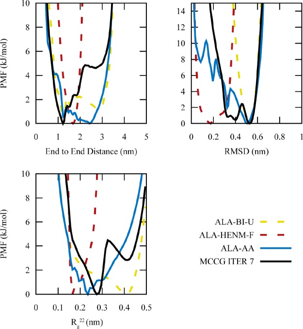
We further analyzed the MCCG trajectories to determine whether ALA-MCCG can accurately capture additional CVs that were not included in the development of the coupling term (Figure 5). For each additional CV, MCCG produces a PMF that is a combination of the ALA-HENM-F and ALA-BI-U models. The two collective variables most correlated with the coupled CVs, R_g²² (the second component of the gyration tensor, which describes the width of the polymer) and RMSD, improve the most compared with the 1D AA PMFs. However, end-to-end distance, which is least correlated with the coupled CVs, is worse at reproducing the reference AA PMF. This demonstrates the importance of choosing good (or possibly additional) CVs for the MCCG coupling term. CVs not as correlated with the coupled CVs (or anticorrelated) may potentially be adversely affected by the MCCG procedure. By reducing the many-body PMF to a PMF dependent only upon a few CVs, some information is inevitably lost. Choosing CVs that can best represent the many-body PMF in the full set of CG variables R^N will produce the best MCCG models, but there is obviously a limit on how many CVs can be chosen in terms of one’s ability to calculate the AA multidimensional reduced PMFs as a function of them (here, we have used 2D PMFs). Thus, when building MCCG models, it is important to check whether other PMF properties not correlated with the coupled CVs are affected.

Figure 5.

1D PMFs for three CVs comparing the ALA MCCG model with all-atom PMFs, as well as the two CG models comprising the MCCG model. The MCCG model more accurately represents CVs that are coupled (RMSD) or correlated with the coupled CVs (R_g²²). CVs that are not related to the coupled CVs (end-to-end distance) are less accurately captured.

Endophilin H0

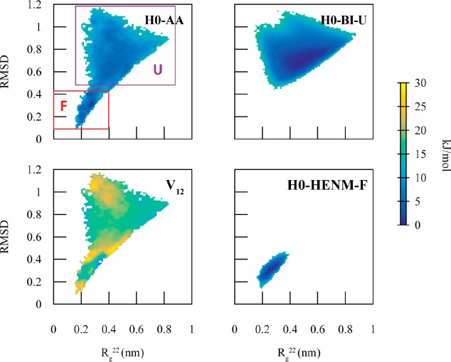
The folding process of endophilin H0, a 22-residue amphipathic helix that targets curved membranes, has been previously studied by Cui et al.⁵⁶ The folding process was characterized using the α–β similarity and the number of backbone hydrogen bonds CVs. These CVs can only be described using atomistic detail. Here, we chose to characterize the folding process using the root mean squared deviation (RMSD) from the idealized folded configuration and the second component of the gyration tensor⁵⁷ (R_g²²) of the Cα coordinates (Figure 6a). These CVs adequately separate the two states and contain a distinct transition region. The folded configuration of H0 is characterized by R_g and RMSD values less than 0.4 nm, while the unfolded configuration is characterized by RMSD > 0.5 nm.

Figure 6.

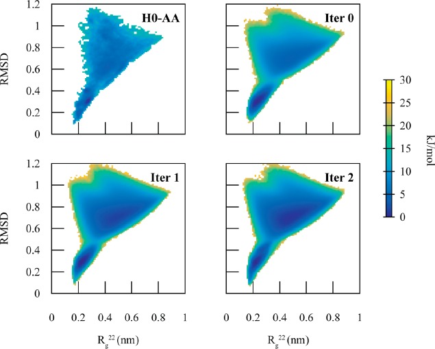
2D PMFs as a function of root mean squared deviation (RMSD) and the second component of the gyration tensor (R_g²²) for H0. For the mapped AA system (H0-AA), the folded state is denoted in the red square (F) and the unfolded state (U), in purple. The Boltzmann inversion CG model of the unfolded state (H0-BI-U) captures the unfolded portion of the AA PMF, and the hENM CG model of the folded state (H0-BI-F) captures the folded portion of the AA PMF. The coupling term (V₁₂(Q)) is at a maximum in the transition region (RMSD = 0.45) as well as the portions of the PMF unsampled by H0-BI-U and H0-HENM-F.

A BI CG model of the unfolded configuration (H0-BI-U) and a HENM model of folded configuration (H0-HENM-F) accurately reproduced, respectively, the unfolded and folded portions of the PMF, along the CVs R_g²² and RMSD, but with smoothed PMF minima compared to the AA PMF. As noted earlier, CG models typically smooth out portions of the free energy surface because the high frequency motions are integrated out of the model. We then constructed an MCCG model of H0 (H0-MCCG). As in the case of dodecaalanine, the coupling is highest in the transition region (Figure 6), as well as regions not sampled by the diabatic states (RMSD > 1.0 nm and RMSD < 0.2 nm).

H0-MCCG exhibits two-state behavior, sampling both the unfolded and folded configurations, with transitions between the two states (Figure 7). H0-MCCG has a barrier height of 10 kJ/mol, within an order of k_BT of the barrier height of 7.5 kJ/mol in the AA PMF. As in the case of dodecalanine, the initial MCCG barrier height is incorrect. Applying the iterative MCCG method for only 2 iterations for H0-MCCG, however, reproduces the 7.5 kJ/mol barrier height at RMSD = 0.5 nm.

Figure 7.

2D PMFs as a function of root mean squared deviation (RMSD) and the second component of the gyration tensor (R_g²²) comparing the mapped AA system (H0-AA) with various iterations (Iter X) of MCCG. The iterative procedure improves the difference in free energy difference between the two states and converges to H0-AA within 2 iterations.

The H0-MCCG PMF is in much better agreement with the AA PMF compared to ALA-MCCG. This is likely caused by the more accurate diabatic states in the case of the H0-MCCG models. The coupling term is therefore required to do less work to reproduce the AA PMF, as it is already more accurately represented by the individual CG models. Accordingly, the number of iterations required to converge the barrier height and PMF minima is significantly reduced due to the improved CG diabatic states.

Conclusions

Proteins can undergo major conformational changes that cannot always be captured by a single CG model having an imperfect description of the interactions between the CG sites. The MCCG method introduced in this work is thus designed to capture the transitions between multiple conformational basins in an approximate CG model in a way that can reasonably reproduce the overall PMF for the conformational change process. Although previous methods have been developed that can simulate a CG model that transitions between multiple conformational states, these methods are not guaranteed to reproduce key features of the AA PMF, especially in the transition barrier region. In contrast, the new MCCG method utilizes an AA-based off-diagonal coupling, the V₁₂(Q) term in eq 6, to reproduce the correct distribution of states as well as the transition barrier.

An important strength of the MCCG method is the fact that the off-diagonal coupling term is defined to be a function of the CVs that describe the transition process. When a constant off-diagonal coupling term is used in contrast, the system may be unable to capture the correct location of the transition barrier, in addition to its height. Using a coupling term that is a function of the transition CVs not only allows the system to reproduce the transition barrier but also leads to a more realistic description of the transition process. Additionally, as the method is applied to other systems, more complicated CVs can be used to incorporate other influences on structural transformations, for example, environmental interactions that affect protein structure. As long as a PMF can be calculated, or at least estimated, to describe the transition between states, whether from AA simulations, from experiment, or phenomenologically, an MCCG model can be parametrized for the system under study.

Another advantage of the MCCG method is the ability to use simple CG models to capture complex, multistate (i.e., multiconformation) behavior in a sort of “divide and conquer” fashion instead of using more complex CG modeling methods. If CG models are constructed and adequate for each of the individual protein conformations, and if the AA PMF (or a good estimate of it) is known for the structural transition, then an MCCG model can be created for the system. An accurate MCCG model may ideally utilize the calculation of the AA PMF, which can be computationally expensive, but for which many methods have been developed.⁵⁸⁻⁶² The major reduction in computational effort afforded by the resulting MCCG model can then be taken advantage of to investigate new emergent behavior. For example, when many proteins are allowed to interact with each other, such as in cellular environments, the MCCG model will be influenced not only by the PMF for a single protein but also by the interactions between proteins on the CG level. This will lead to simulations that will be more representative of actual cellular environments, where protein conformations are influenced both by smaller scale atomic level interactions and by the larger scale protein motions and protein–protein interactions.

The authors declare no competing financial interest.

References

- Schlick T.; Collepardo-Guevara R.; Halvorsen L. A.; Jung S.; Xiao X. Biomolecular Modeling and simulation: a field coming of age. Q. Rev. Biophys. 2011, 44 (2), 191–228. 10.1017/S0033583510000284. [DOI] [PMC free article] [PubMed] [Google Scholar]
- Riniker S.; Allison J. R.; van Gunsteren W. F. On developing coarse-grained models for biomolecular simulation: a review. Phys. Chem. Chem. Phys. 2012, 14 (36), 12423. 10.1039/c2cp40934h. [DOI] [PubMed] [Google Scholar]
- Marrink S. J.; Tieleman D. P. Perspective on the Martini model. Chem. Soc. Rev. 2013, 42 (16), 6801. 10.1039/c3cs60093a. [DOI] [PubMed] [Google Scholar]
- Saunders M. G.; Voth G. A. Coarse-Graining Methods for Computational Biology. Annu. Rev. Biophys. 2013, 42 (1), 73–93. 10.1146/annurev-biophys-083012-130348. [DOI] [PubMed] [Google Scholar]
- Noid W. G. Perspective: Coarse-grained models for biomolecular systems. J. Chem. Phys. 2013, 139 (9), 090901. 10.1063/1.4818908. [DOI] [PubMed] [Google Scholar]
- Grime J. M. A.; Voth G. A. Early Stages of the HIV-1 Capsid Protein Lattice Formation. Biophys. J. 2012, 103 (8), 1774–1783. 10.1016/j.bpj.2012.09.007. [DOI] [PMC free article] [PubMed] [Google Scholar]
- Globisch C.; Krishnamani V.; Deserno M.; Peter C. Optimization of an Elastic Network Augmented Coarse Grained Model to Study CCMV Capsid Deformation. PLoS One 2013, 8 (4), e60582 10.1371/journal.pone.0060582. [DOI] [PMC free article] [PubMed] [Google Scholar]
- Pak A. J.; Grime J. M. A.; Sengupta P.; Chen A. K.; Durumeric A. E. P.; Srivastava A.; Yeager M.; Briggs J. A. G.; Lippincott-Schwartz J.; Voth G. A. Immature HIV-1 lattice assembly dynamics are regulated by scaffolding from nucleic acid and the plasma membrane. Proc. Natl. Acad. Sci. U. S. A. 2017, 114 (47), E10056–E10065. 10.1073/pnas.1706600114. [DOI] [PMC free article] [PubMed] [Google Scholar]
- Simunovic M.; Evergren E.; Golushko I.; Prévost C.; Renard H.-F.; Johannes L.; McMahon H. T.; Lorman V.; Voth G. A.; Bassereau P. How curvature-generating proteins build scaffolds on membrane nanotubes. Proc. Natl. Acad. Sci. U. S. A. 2016, 113 (40), 11226–11231. 10.1073/pnas.1606943113. [DOI] [PMC free article] [PubMed] [Google Scholar]
- Simunovic M.; Srivastava A.; Voth G. A. Linear aggregation of proteins on the membrane as a prelude to membrane remodeling. Proc. Natl. Acad. Sci. U. S. A. 2013, 110 (51), 20396–20401. 10.1073/pnas.1309819110. [DOI] [PMC free article] [PubMed] [Google Scholar]
- Simunovic M.; Voth G. A. Membrane tension controls the assembly of curvature-generating proteins. Nat. Commun. 2015, 6 (1), 7219. 10.1038/ncomms8219. [DOI] [PMC free article] [PubMed] [Google Scholar]
- Simunovic M.; Voth G. A.; Callan-Jones A.; Bassereau P. When Physics Takes Over: BAR Proteins and Membrane Curvature. Trends Cell Biol. 2015, 25 (12), 780–792. 10.1016/j.tcb.2015.09.005. [DOI] [PMC free article] [PubMed] [Google Scholar]
- Su J.; Thomas A. S.; Grabietz T.; Landgraf C.; Volkmer R.; Marrink S. J.; Williams C.; Melo M. N. The N-terminal amphipathic helix of Pex11p self-interacts to induce membrane remodelling during peroxisome fission. Biochim. Biophys. Acta, Biomembr. 2018, 1860 (6), 1292–1300. 10.1016/j.bbamem.2018.02.029. [DOI] [PubMed] [Google Scholar]
- Fuhrmans M.; Marrink S. J. Molecular view of the role of fusion peptides in promoting positive membrane curvature. J. Am. Chem. Soc. 2012, 134 (3), 1543–1552. 10.1021/ja207290b. [DOI] [PubMed] [Google Scholar]
- Braun A. R.; Sevcsik E.; Chin P.; Rhoades E.; Tristram-Nagle S.; Sachs J. N. α-Synuclein induces both positive mean curvature and negative Gaussian curvature in membranes. J. Am. Chem. Soc. 2012, 134 (5), 2613–2620. 10.1021/ja208316h. [DOI] [PMC free article] [PubMed] [Google Scholar]
- Arkhipov A.; Yin Y.; Schulten K. Four-scale description of membrane sculpting by BAR domains. Biophys. J. 2008, 95 (6), 2806–2821. 10.1529/biophysj.108.132563. [DOI] [PMC free article] [PubMed] [Google Scholar]
- Lelimousin M.; Limongelli V.; Sansom M. S. P. Conformational changes in the epidermal growth factor receptor: Role of the transmembrane domain investigated by coarse-grained MetaDynamics free energy calculations. J. Am. Chem. Soc. 2016, 138 (33), 10611–10622. 10.1021/jacs.6b05602. [DOI] [PMC free article] [PubMed] [Google Scholar]
- Calero-Rubio C.; Paik B.; Jia X.; Kiick K. L.; Roberts C. J. Predicting unfolding thermodynamics and stable intermediates for alanine-rich helical peptides with the aid of coarse-grained molecular simulation. Biophys. Chem. 2016, 217, 8–19. 10.1016/j.bpc.2016.07.002. [DOI] [PMC free article] [PubMed] [Google Scholar]
- Rudzinski J. F.; Bereau T. Concurrent parametrization against static and kinetic information leads to more robust coarse-grained force fields. Eur. Phys. J.: Spec. Top. 2016, 225 (8–9), 1373–1389. 10.1140/epjst/e2016-60114-5. [DOI] [Google Scholar]
- Monticelli L.; Kandasamy S. K.; Periole X.; Larson R. G.; Tieleman D. P.; Marrink S.-J. The MARTINI coarse-grained force field: Extension to proteins. J. Chem. Theory Comput. 2008, 4 (5), 819–834. 10.1021/ct700324x. [DOI] [PubMed] [Google Scholar]
- de Jong D. H.; Singh G.; Bennett W. F.; Arnarez C.; Wassenaar T. A.; Schafer L. V.; Periole X.; Tieleman D. P.; Marrink S. J. Improved parameters for the Martini coarse-grained protein force field. J. Chem. Theory Comput. 2013, 9 (1), 687–97. 10.1021/ct300646g. [DOI] [PubMed] [Google Scholar]
- Periole X.; Cavalli M.; Marrink S.-J.; Ceruso M. A. Combining an elastic network with a coarse-grained molecular force field: Structure, dynamics, and intermolecular recognition. J. Chem. Theory Comput. 2009, 5 (9), 2531–2543. 10.1021/ct9002114. [DOI] [PubMed] [Google Scholar]
- Chebaro Y.; Pasquali S.; Derreumaux P. The Coarse-Grained OPEP Force Field for Non-Amyloid and Amyloid Proteins. J. Phys. Chem. B 2012, 116 (30), 8741–8752. 10.1021/jp301665f. [DOI] [PubMed] [Google Scholar]
- Shell M. S. The relative entropy is fundamental to multiscale and inverse thermodynamic problems. J. Chem. Phys. 2008, 129 (14), 144108. 10.1063/1.2992060. [DOI] [PubMed] [Google Scholar]
- Izvekov S.; Voth G. A. A Multiscale Coarse-Graining Method for Biomolecular Systems. J. Phys. Chem. B 2005, 109 (7), 2469–2473. 10.1021/jp044629q. [DOI] [PubMed] [Google Scholar]
- Noid W. G.; Chu J.-W.; Ayton G. S.; Krishna V.; Izvekov S.; Voth G. A.; Das A.; Andersen H. C. The multiscale coarse-graining method. I. A rigorous bridge between atomistic and coarse-grained models. J. Chem. Phys. 2008, 128 (24), 244114. 10.1063/1.2938860. [DOI] [PMC free article] [PubMed] [Google Scholar]
- Noid W. G.; Liu P.; Wang Y.; Chu J.-W.; Ayton G. S.; Izvekov S.; Andersen H. C.; Voth G. A. The multiscale coarse-graining method. II. Numerical implementation for coarse-grained molecular models. J. Chem. Phys. 2008, 128 (24), 244115. 10.1063/1.2938857. [DOI] [PMC free article] [PubMed] [Google Scholar]
- Thorpe I. F.; Zhou J.; Voth G. A. Peptide folding using multiscale coarse-grained models. J. Phys. Chem. B 2008, 112 (41), 13079–13090. 10.1021/jp8015968. [DOI] [PubMed] [Google Scholar]
- Carmichael S. P.; Shell M. S. A new multiscale algorithm and its application to coarse-grained peptide models for self-assembly. J. Phys. Chem. B 2012, 116 (29), 8383–93. 10.1021/jp2114994. [DOI] [PubMed] [Google Scholar]
- Rudzinski J. F.; Noid W. G. Bottom-up coarse-graining of peptide ensembles and helix–coil transitions. J. Chem. Theory Comput. 2015, 11 (3), 1278–1291. 10.1021/ct5009922. [DOI] [PubMed] [Google Scholar]
- Pollard T. D.; Blanchoin L.; Mullins R. D. Molecular mechanisms controlling actin filament dynamics in nonmuscle cells. Annu. Rev. Biophys. Biomol. Struct. 2000, 29 (1), 545–576. 10.1146/annurev.biophys.29.1.545. [DOI] [PubMed] [Google Scholar]
- Maragakis P.; Karplus M. Large amplitude conformational change in proteins explored with a plastic network model: Adenylate kinase. J. Mol. Biol. 2005, 352 (4), 807–822. 10.1016/j.jmb.2005.07.031. [DOI] [PubMed] [Google Scholar]
- Okazaki K. i.; Koga N.; Takada S.; Onuchic J. N.; Wolynes P. G. Multiple-basin energy landscapes for large-amplitude conformational motions of proteins: Structure-based molecular dynamics simulations. Proc. Natl. Acad. Sci. U. S. A. 2006, 103 (32), 11844–11849. 10.1073/pnas.0604375103. [DOI] [PMC free article] [PubMed] [Google Scholar]
- Chu J.-W.; Voth G. A. Coarse-grained free energy functions for studying protein conformational changes: A double-well network model. Biophys. J. 2007, 93 (11), 3860–3871. 10.1529/biophysj.107.112060. [DOI] [PMC free article] [PubMed] [Google Scholar]
- Zheng W.; Brooks B. R.; Hummer G. Protein conformational transitions explored by mixed elastic network models. Proteins: Struct., Funct., Genet. 2007, 69 (1), 43–57. 10.1002/prot.21465. [DOI] [PubMed] [Google Scholar]
- de Marco G.; Várnai P. Molecular simulation of conformational transitions in biomolecules using a combination of structure-based potential and empirical valence bond theory. Phys. Chem. Chem. Phys. 2009, 11 (45), 10694. 10.1039/b917109f. [DOI] [PubMed] [Google Scholar]
- Bereau T.; Rudzinski J. F. Accurate Structure-Based Coarse Graining Leads to Consistent Barrier-Crossing Dynamics. Phys. Rev. Lett. 2018, 121 (25), 256002. 10.1103/PhysRevLett.121.256002. [DOI] [PubMed] [Google Scholar]
- Marcus R. A. Chemical and electrochemical electron-transfer theory. Annu. Rev. Phys. Chem. 1964, 15 (1), 155–196. 10.1146/annurev.pc.15.100164.001103. [DOI] [Google Scholar]
- Warshel A.; Weiss R. M. An empirical valence bond approach for comparing reactions in solutions and in enzymes. J. Am. Chem. Soc. 1980, 102 (20), 6218–6226. 10.1021/ja00540a008. [DOI] [Google Scholar]
- Chang Y. T.; Miller W. H. An empirical valence bond model for constructing global potential energy surfaces for chemical reactions of polyatomic molecular systems. J. Phys. Chem. 1990, 94 (15), 5884–5888. 10.1021/j100378a052. [DOI] [Google Scholar]
- Abraham M. J.; Murtola T.; Schulz R.; Páll S.; Smith J. C.; Hess B.; Lindahl E. GROMACS: High performance molecular simulations through multi-level parallelism from laptops to supercomputers. SoftwareX 2015, 1–2, 19–25. 10.1016/j.softx.2015.06.001. [DOI] [Google Scholar]
- Best R. B.; Zhu X.; Shim J.; Lopes P. E.; Mittal J.; Feig M.; Mackerell A. D. Jr. Optimization of the additive CHARMM all-atom protein force field targeting improved sampling of the backbone phi, psi and side-chain chi(1) and chi(2) dihedral angles. J. Chem. Theory Comput. 2012, 8 (9), 3257–3273. 10.1021/ct300400x. [DOI] [PMC free article] [PubMed] [Google Scholar]
- Essmann U.; Perera L.; Berkowitz M. L.; Darden T.; Lee H.; Pedersen L. G. A smooth particle mesh Ewald method. J. Chem. Phys. 1995, 103 (19), 8577–8593. 10.1063/1.470117. [DOI] [Google Scholar]
- Hess B. P-LINCS: A parallel linear constraint solver for molecular simulation. J. Chem. Theory Comput. 2008, 4 (1), 116–22. 10.1021/ct700200b. [DOI] [PubMed] [Google Scholar]
- Bussi G.; Donadio D.; Parrinello M. Canonical sampling through velocity rescaling. J. Chem. Phys. 2007, 126 (1), 014101. 10.1063/1.2408420. [DOI] [PubMed] [Google Scholar]
- Parrinello M.; Rahman A. Polymorphic transitions in single crystals: A new molecular dynamics method. J. Appl. Phys. 1981, 52 (12), 7182–7190. 10.1063/1.328693. [DOI] [Google Scholar]
- Humphrey W.; Dalke A.; Schulten K. VMD: visual molecular dynamics. J. Mol. Graphics 1996, 14 (1), 27–38. 10.1016/0263-7855(96)00018-5. [DOI] [PubMed] [Google Scholar]
- Sugita Y.; Okamoto Y. Replica-exchange molecular dynamics method for protein folding. Chem. Phys. Lett. 1999, 314 (1–2), 141–151. 10.1016/S0009-2614(99)01123-9. [DOI] [Google Scholar]
- Plimpton S. Fast parallel algorithms for short-range molecular dynamics. J. Comput. Phys. 1995, 117 (1), 1–19. 10.1006/jcph.1995.1039. [DOI] [Google Scholar]
- Schneider T.; Stoll E. Molecular-dynamics study of a three-dimensional one-component model for distortive phase transitions. Phys. Rev. B: Condens. Matter Mater. Phys. 1978, 17 (3), 1302–1322. 10.1103/PhysRevB.17.1302. [DOI] [Google Scholar]
- Tribello G. A.; Bonomi M.; Branduardi D.; Camilloni C.; Bussi G. PLUMED 2: New feathers for an old bird. Comput. Phys. Commun. 2014, 185 (2), 604–613. 10.1016/j.cpc.2013.09.018. [DOI] [Google Scholar]
- Lyman E.; Pfaendtner J.; Voth G. A. Systematic multiscale parameterization of heterogeneous elastic network models of proteins. Biophys. J. 2008, 95 (9), 4183–4192. 10.1529/biophysj.108.139733. [DOI] [PMC free article] [PubMed] [Google Scholar]
- Tozzini V.; Rocchia W.; McCammon J. A. Mapping all-atom models onto one-bead coarse-grained models: General properties and applications to a minimal polypeptide model. J. Chem. Theory Comput. 2006, 2 (3), 667–673. 10.1021/ct050294k. [DOI] [PMC free article] [PubMed] [Google Scholar]
- Cho H. M.; Chu J. W. Inversion of radial distribution functions to pair forces by solving the Yvon-Born-Green equation iteratively. J. Chem. Phys. 2009, 131 (13), 134107. 10.1063/1.3238547. [DOI] [PubMed] [Google Scholar]
- Lu L.; Dama J. F.; Voth G. A. Fitting coarse-grained distribution functions through an iterative force-matching method. J. Chem. Phys. 2013, 139 (12), 121906. 10.1063/1.4811667. [DOI] [PubMed] [Google Scholar]
- Cui H.; Mim C.; Vázquez F. X.; Lyman E.; Unger V. M.; Voth G. A. Understanding the role of amphipathic helices in N-BAR domain driven membrane remodeling. Biophys. J. 2013, 104 (2), 404–411. 10.1016/j.bpj.2012.12.006. [DOI] [PMC free article] [PubMed] [Google Scholar]
- Vymetal J.; Vondrasek J. Gyration- and inertia-tensor-based collective coordinates for metadynamics. Application on the conformational behavior of polyalanine peptides and Trp-cage folding. J. Phys. Chem. A 2011, 115 (41), 11455–65. 10.1021/jp2065612. [DOI] [PubMed] [Google Scholar]
- Darve E.; Rodriguez-Gomez D.; Pohorille A. Adaptive biasing force method for scalar and vector free energy calculations. J. Chem. Phys. 2008, 128 (14), 144120. 10.1063/1.2829861. [DOI] [PubMed] [Google Scholar]
- Torrie G. M.; Valleau J. P. Nonphysical sampling distributions in Monte Carlo free-energy estimation: Umbrella sampling. J. Comput. Phys. 1977, 23 (2), 187–199. 10.1016/0021-9991(77)90121-8. [DOI] [Google Scholar]
- Laio A.; Parrinello M. Escaping free-energy minima. Proc. Natl. Acad. Sci. U. S. A. 2002, 99 (20), 12562–12566. 10.1073/pnas.202427399. [DOI] [PMC free article] [PubMed] [Google Scholar]
- Barducci A.; Bussi G.; Parrinello M. Well-tempered Metadynamics: A smoothly converging and tunable free-energy method. Phys. Rev. Lett. 2008, 100 (2), 020603. 10.1103/PhysRevLett.100.020603. [DOI] [PubMed] [Google Scholar]
- Dama J. F.; Rotskoff G.; Parrinello M.; Voth G. A. Transition-Tempered Metadynamics: Robust, Convergent Metadynamics via On-the-Fly Transition Barrier Estimation. J. Chem. Theory Comput. 2014, 10 (9), 3626–33. 10.1021/ct500441q. [DOI] [PubMed] [Google Scholar]