Red fox genome assembly identifies genomic regions associated with tame and aggressive behaviors

Abstract

Strains of red fox (Vulpes vulpes) with markedly different behavioral phenotypes have been developed in the famous long-term selective breeding program known as the Russian farm-fox experiment. Here we sequenced and assembled the red fox genome and re-sequenced a subset of foxes from the tame, aggressive, and conventional farm-bred populations to identify genomic regions associated with the response to selection for behavior. Analysis of the resequenced genomes identified 103 regions with either significantly decreased heterozygosity in one of the three populations or increased divergence between the populations. A strong positional candidate gene for tame behavior was highlighted: SorCS1, which encodes the main trafficking protein for AMPA glutamate receptors and neurexins and suggests a role for synaptic plasticity in fox domestication. Other regions identified as likely to have been under selection in foxes during domestication include genes implicated in human neurological disorders, mouse behavior, and dog domestication. The fox represents a powerful model for the genetic analysis of affiliative and aggressive behaviors that can benefit genetic studies of behavior in dogs and other mammals, including humans.

The red fox (Vulpes vulpes) and the domestic dog (Canis familiaris) are closely related species that diverged only about 10 million years ago within the family Canidae¹. However, these two species occupy very different ecological niches. The red fox has a geographic range wider than that of any other wild species in the order Carnivora² and has even become a common resident of many major cities^3–6. The dog, on the other hand, has become widespread for a different reason: it was domesticated from the gray wolf at least 15,000 years ago^7,8 and became “man’s best friend.”

There is no evidence that the fox was domesticated historically, although a red fox was found co-buried with humans in a Natufian grave from 14.5–11.6 KYA at a southern Levant site in northern Jordan⁹, the same geographic region where the oldest co-burials of humans and dogs are found¹⁰. The first strong evidence of fox domestication comes instead from the late 19th century, when the farm breeding of red foxes for fur began in Prince Edward Island, Canada¹¹. Though many animal species are not well-suited to breeding in captivity¹², fox breeding has continued successfully for more than a century^11,13–17. Conventional farm-bred foxes have adapted to the farm environment, yet their behavior still clearly differentiates them from dogs because they generally exhibit fear or aggression toward humans.

In 1959, the experimental domestication of farm-bred foxes began at the Institute of Cytology and Genetics of the Russian Academy of Sciences^18–23. For over 50 generations, foxes were selected for positive responses toward humans, leading to the establishment of a tame strain of foxes that are eager to interact with humans from a very young age^21,24. Beginning in the late 1960s, a complementary strain of foxes selected for aggressive behavior toward humans was also developed and has proceeded for more than 40 generations^22,23. A conventional population comparable to the farm-bred founder population of both selected strains has also been maintained but was not subjected to deliberate selection for behavior. The fox strains have remained outbred during the entire course of the breeding program, and a strong genetic contribution to the behavioral differences between the tame and aggressive strains has been confirmed^20,23,25,26. Unlike modern dogs, which have been selected for a wide variety of traits, these fox strains were selected solely for behavior, and the shifts in their behavior were recent and well documented.

Maximizing the scientific value of these experimental fox populations requires the development of genomic tools for the fox. In contrast to the dog, whose karyotype consists of 38 pairs of acrocentric autosomes in addition to the sex chromosomes, the red fox karyotype comprises 16 pairs of metacentric autosomes, the sex chromosomes, and 0–8 supernumerary B chromosomes^27,28. Synteny between the dog and fox chromosomes has been established but at a low resolution^29–33, hindering identification of the regions in the dog genome that correspond to genomic regions of interest in the fox.

Here, we present the sequence assembly of the red fox genome and a population genetic analysis of whole re-sequenced genomes of foxes from the tame, aggressive, and conventional farm-bred populations. Selection on the tame and aggressive strains is likely to have influenced genetic diversity and the fixation of variants across the genome, yielding a robust model for understanding the genetic basis of variation in social behavior, which is a long-standing problem in evolutionary biology.

Results

The red fox genome assembly and annotation.

A male red fox with a standard karyotype (Supplementary Figure 1) was sequenced to 93.9x coverage using Illumina HiSeq and assembled with SOAPdenovo V2.04.4³⁴. The genome comprises 676,878 scaffolds (scaffold N50 is 11,799,617 bp) and includes 21,418 annotated fox protein coding genes (Supplementary Tables 1, 2).

Alignment of the largest 500 scaffolds against the dog genome revealed that 84% of the scaffolds mapped to one dog chromosome, 15% mapped to two or more dog chromosomes, and 1% could not be assigned to a position in the dog genome (Supplementary Table 3; Supplementary Figure 2). Among the scaffolds that mapped to more than one dog chromosome, five mapped to two dog chromosomes that are known to be syntenic to a single fox chromosome^29–32,35.

Genetic structure of fox populations.

The genomes of 10 foxes from each of the three populations (tame, aggressive, and conventional farm-bred) were sequenced with a coverage of ~2.5x, yielding ~75x total genome coverage across all 30 animals (Supplementary Table 4). The 96% of the reads were aligned to the fox scaffolds and the 8,458,133 identified SNPs were retained for subsequent analyses (Supplementary Table 5). The assessment of the relationship among 30 individuals using principal component analysis, neighbor-joining analysis³⁶, and STRUCTURE 2.3.4^37–40 indicated the presence of three populations in the data set and less divergence between the conventional and aggressive populations than between the tame and either the conventional or aggressive population (Figure 1).

Figure 1. Principal component analysis (a), neighbor-joining tree analysis (b), and STRUCTURE analysis (c) of the fox populations.

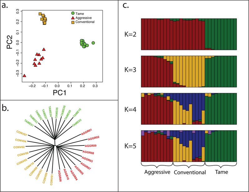
All analyses were performed using SNP data for 30 foxes (10 each from the tame, aggressive and conventional populations) whose genomes were re-sequenced. In figures a and b, each individual is represented by shape (a) or line (b). In figure c, each individual is represented by a bar that is segmented into colors based on its assignment into inferred clusters given the assumption of k populations. The length of the colored segment is the estimated proportion of the individual’s genome belonging to that cluster. Each level of k was run 4 times, but the data shown is from the run giving the highest estimated probability of observing the data. The assumed number of clusters (k) is indicated on the y-axis. The population origin of individuals is indicated on the x-axis.

Genomic regions differentiating fox populations.

Simulations were performed in order to support the identification of genomic regions targeted by selection rather than genetic drift (Supplementary Note 1; Supplementary Figures 3–6). To identify regions of complete or nearly complete fixation within each of the three populations, pooled heterozygosity (Hp) was estimated. Hp was calculated for 9,151 windows of 500 kb that were moved along the genome in 250-kb steps. Population-specific cut-offs corresponding to p<0.0001 revealed 96 low-Hp windows in the tame (HpT), 60 windows in the aggressive (HpA) and 14 windows in the conventional population (HpC) (Figure 2; Supplementary Tables 6, 7). None of the identified HpT windows overlapped with the HpA and HpC windows, but two Hp windows were significant in both the aggressive and conventional populations. In total, 138 annotated genes were found in HpT windows, 159 in HpA windows, and 51 in HpC windows (Supplementary Tables 7, 8).

Figure 2. Genome-wide fixation index (F_ST) and Pooled Heterozygosity (Hp) analyses across the fox genome.

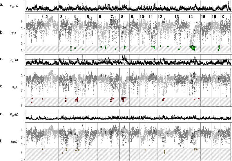
Dots on all panels represent the 500-kb windows analyzed in both the F_ST and Hp analyses. The order of the windows is based on the LASTZ mapping of individual windows to the dog genome and the previously published fox/dog synteny map (chimeric scaffolds are split to reflect the most likely location of each window in the fox genome). Gray vertical lines separate fox chromosomes. Chromosome numbers are indicated in panel b. Panels a, c, and e: F_ST analysis across the fox genome. The horizontal line is F_ST =0.458. Panels b, e, and f: Hp analysis across the fox genome. The gray patterned box and colored dots indicate the windows that reached significance in that population (Supplementary Table 6; Supplementary Figure 11). The dots that are outlined in the non-significant zones are windows that reached significance in a different population. a. F_ST between the tame and conventional populations. b. Hp in the tame population. c. F_ST between tame and aggressive populations. d. Hp in the aggressive population. e. F_ST between aggressive and conventional populations. f. Hp in the conventional population.

Fixation index (F_ST) was calculated for the same 9,151 windows used in the Hp analyses to identify regions of extreme differentiation between the fox populations. Only 3% of windows in the analysis of the tame and aggressive populations had F_ST values of 0.458 or higher. Using an F_ST value of 0.458 as a cut-off for significance (Supplementary Note 2), we identified 275 windows in the analysis of the tame and aggressive populations (F_STTA), 106 windows in the analysis of the tame and conventional populations (F_STTC), and 1 window in the analysis of the aggressive and conventional populations (F_STAC) (Supplementary Table 7; Figure 2). In total, 650 annotated genes are located in the identified F_STTA windows, 234 in F_STTC windows, and three in F_STAC windows. Among the identified F_ST windows, 18.7% were also significant in the Hp analysis, and 35.7% of significant Hp windows were significant in the F_ST analysis (Supplementary Tables 7, 8).

PANTHER overrepresentation analysis⁴¹ (Supplementary Table 9) identified significant enrichment for the GO term “carbohydrate binding” in the HpA and F_STTA windows as well as terms related to “clathrin-coated vesicle” and the immune response, specifically “cytokine activity” (HpA) and “interleukin-1 receptor binding” (F_STTA). The analysis of the HpT windows identified enrichment for “single guanine insertion binding,” and “damaged DNA binding”. Other terms identified in the F_STTA, F_STTC, and F_STAC windows are presented in Supplementary Table 9.

More than 80% of genes located in the 9,151 windows were found to be brain-expressed and no overrepresentation for brain-expressed genes in the significant windows was observed (Supplementary Table 10). Several receptor-coding genes for glutamatergic (GRIN2B, GRM6), GABAergic (GABBR1, GABRA3, GABRQ), and cholinergic (CHRM3, CHRNA7) synapses have been identified among the genes located in significant windows (Supplementary Table 11).

To avoid splitting a single sweep across multiple windows, significant Hp windows located close to each other were merged, yielding 30, 19, and 10 combined Hp windows in the tame, aggressive, and conventional populations, respectively. Although most of the combined windows were comprised by one to five windows, two combined HpT windows and two combined HpA windows were longer than 5 Mb (Supplementary Tables 7, 12; Supplementary Figure 7).

The same rule was used to merge significant F_ST windows and produced 57 combined F_STTA windows, 42 combined F_STTC windows, and one combined F_STAC window (Supplementary Table 7; Supplementary Figure 7). Among the six combined F_STTA windows that were 5 Mb or larger, one overlaps completely with a large combined HpT window (VVU14, region 86), and two overlap completely (VVU4, region 27) or partially (VVU8, region 46) with large combined HpA windows.

The analysis of the positions of all significant windows revealed 103 regions in the fox genome (Supplementary Table 7). The comparison of these regions to the regions associated with domestication and positive selection in dogs^42–45 highlighted 45 fox regions. Three candidate domestication regions (CDR) identified in vonHoldt et al.⁴⁴, ten CDRs identified in Axelsson et al.⁴², 22 regions of positive selection in dogs identified in Freedman et al.⁴³, and 38 regions identified in Wang et al.⁴⁵ overlap or are located near the genomic regions identified in foxes (Supplementary Table 13). A tentative enrichment of fox regions for CDRs and regions of positive selection in dogs was observed (p=0.06).

Previous genetic mapping studies using cross-bred fox pedigrees identified nine fox behavioral QTL^26,46. Comparison of the QTL intervals with the positions of the 103 genomic regions from Supplementary Table 7 revealed 30 regions that overlap with five of the QTL (Supplementary Table 14). The identified overlap is significantly higher (p<0.0001) than expected by chance.

Behavior-related genes.

Identification of genes involved in aggression, sociability, and anxiety in foxes is of particular interest because these behaviors are hallmarks of several human behavioral disorders. Analysis of the 971 annotated genes located within significant windows detected 13 genes associated with autism spectrum disorder⁴⁷, 13 genes associated with bipolar disorder⁴⁸, and three genes located at the border of the Williams-Beuren syndrome deletion in humans⁴⁹ (Supplementary Tables 15, 16). Six genes from the fox regions have been previously associated with aggressive behavior in mice^50,51 (Supplementary Table 15). The analysis of significant windows also highlighted fox genes that are not direct orthologs of human genes associated with behavioral disorders or of mouse genes for aggression but that belong to the same gene families and may have similar functions.

Several behavior-associated genes in significant regions contained alleles corresponding to missense mutations with differences in frequency among the populations (Supplementary Tables 17, 18). Two missense mutations in the autism-associated CACNA1C gene, CACNA1C-SNP1 (Ile937Thr) and CACNA1C-SNP2 (Thr1875Ile), are located at evolutionarily conserved sites and the CACNA1C-SNP1 was predicted by PolyPhen-2 v2.2.2r398⁵² to be “possibly damaging” (score: 0.614; sensitivity: 0.87; specificity: 0.91). The derived fox-specific allele for CACNA1C-SNP1 was observed only in the tame population. In contrast, for CACNA1C-SNP2, the derived allele was observed in both the aggressive and conventional populations but not in the tame population (Supplementary Figure 8).

SorCS1 is a positional candidate for the QTL on fox chromosome 15.

From the 103 regions of interest identified in the fox genome, the 30 regions that overlapping the behavioral QTL mapped in fox pedigrees^26,46 should represent the most likely targets of selection for behavior in the tame and aggressive populations (Supplementary Table 14). To test this assumption, we analyzed an identified genomic region (region 94 on scaffold 1) that is located on VVU15 within the fox QTL interval (Supplementary Table 14; Figure 3). Region 94 incudes a single significant F_STTA window that corresponds to part of the SorCS1 gene (Supplementary Tables 7, 18). Although this window did not reach the significance thresholds for Hp in the tame (HpT=0.20) and aggressive (HpA=0.23) populations, the likelihood of observing such extreme Hp values is low (tame p<0.005; aggressive p<0.001).

Figure 3. SorCS1 region on VVU15.

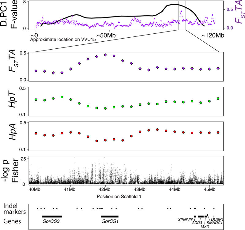
The top panel represents the QTL plot for D.PC1 (black line) and the distribution of F_ST values (purple) between the tame and aggressive populations. The position on VVU15 is approximated by adding the lengths of the portions of the scaffolds that mapped to the syntenic dog chromosomes (CFA31, CFA28). The three lower panels show the F_ST and Hp values on fox scaffold 1: 40–45Mb, the segment that maps to the region on VVU15 (CFA28 segment) that has the QTL for D.PC1 and a significant hit for F_ST between the tame and aggressive populations. The fifth panel shows the results of the Fisher exact tests for allele frequency differences between the tame and aggressive populations conducted using individual SNPs. The x-axis is the –log10 transformed unadjusted p-values. The bottom panel shows the positions of the genes in the region (black lines) and all genotyped markers (black dots).

The QTL on VVU15 was identified for the behavioral phenotype D.PC1 (a phenotype defined using principal component analysis) that differentiates foxes that continue to solicit an observer’s attention after an interaction (higher D.PC1) versus foxes that avoid the observer in the same context (lower D.PC1)⁴⁶. The QTL on VVU15 explains 2.85% of D.PC1 variance in the F2 population⁴⁶.

To test whether inheritance of certain SorCS1 haplotypes predicts variation in D.PC1, we developed 25 short insertion/deletion markers distributed relatively equally across a 5-Mb interval that includes region 94 in the middle (Supplementary Table 19). The markers were genotyped in an additional sample of tame and aggressive foxes and in the F2 pedigrees, whose offspring demonstrate a wide spectrum of behaviors. We analyzed the genotypes of the tame and aggressive foxes to identify the most common haplotypes in the two populations and then tested the effect of the identified haplotypes on behavior in the F2 population.

Haplotype analysis of the tame population identified eight markers located within or in close proximity to the SorCS1 gene (scaffold1: 41,647,754–42,312,608 bp) as a single linkage disequilibrium (LD) block located in the middle of the genotyped 5-Mb interval (Supplementary Figure 9). Within this LD block, Haploview⁵³ identified one haplotype (olv) with a frequency of 60.6% in the tame population that was not observed in the aggressive population, two haplotypes (trq and lav) that were rare in tame but frequent in the aggressive population, and a fourth haplotype (pch) that was found in both populations (Table 1; Figure 4a; Supplementary Table 20). There were four additional uncommon haplotypes that did not reach 10% frequency in either population. Differences in the behavior of F2 individuals homozygous for any of the three main haplotypes (olv, trq, and lav) were statistically significant (Kruskal-Wallis, p=0.03). F2 individuals that inherited two copies of the tame haplotype (olv) had the highest values for D.PC1 (mean: 0.068), while individuals that inherited two copies of one of the common aggressive haplotypes (lav) had the lowest values (mean: −0.546) (Table 1; Figure 4b; Supplementary Figure 10). A post-hoc Dunn’s test with Benjamini-Hochberg⁵⁴ correction achieved a p=0.0142 for the comparison of the lav and olv homozygotes (Figure 4b), while other pair-wise comparisons of homozygotes for the main haplotypes were not significant (p>0.2). Analysis of haplotypes for markers located on the left (5’) and right (3’) ends of the genotyped 5-Mb interval did not identify haplotypes with a significant effect on D.PC1 values in the F2 population (Supplementary Note 3). Significant allele frequency differences for SorCS1 SNPs were also identified in the genotyping-by-sequencing experiment⁵⁵ that used a different sample of the tame and aggressive foxes. Taken together, these data strongly suggest that SorCS1 is a positional candidate for the behavioral QTL on VVU15.

Table 1. Major SorCS1 haplotypes.

The major haplotypes that were found in each of the three regions within the genotyped 5-Mb interval surrounding SorSC1 (left of SorCS1, at SorCS1 (middle), and right of SorCS1). Only haplotypes that reached 10% frequency in at least one of the two populations are shown. The haplotype names in column one are the same names listed in Supplementary Table 20, which contains extended information about the haplotypes found. The frequencies in the tame and aggressive populations are based on the data from Haploview. The number of homozygotes in the F2 population is listed, along with the mean value and variance for D.PC1 in the homozygous individuals. The cumulative distribution of D.PC1 values in F2 homozygotes for the haplotypes in the three regions is shown in Supplementary Figure 10.

Haplotype	Frequency in Tame	Frequency in Aggressive	Number of homozygotes in F2	Mean D.PC1 in F2	Variance D.PC1 in F2
SorCS1 region
trq	7%	47%	15	−0.29	0.64
lav	2%	37%	40	−0.55	1.06
olv	61%	0%	50	0.07	0.95
pch	16%	10%	7	−0.53	1.23
Left of SorCS1
re	19%	33%	35	−0.14	1.17
gr	20%	31%	37	−0.03	0.95
yl	40%	0%	26	−0.39	1.14
Right of SorCS1
p	17%	29%	61	−0.50	1.14
s	51%	10%	17	−0.09	0.77

Figure 4. The SorCS1-associated haplotypes and their effect on behavior in the F2 population.

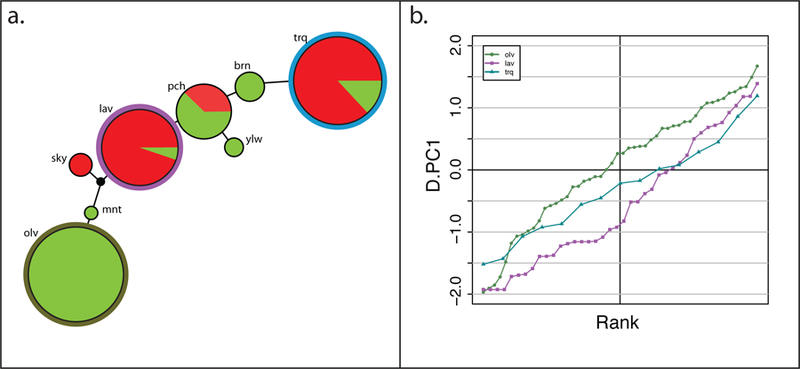
a. A network of the SorCS1 associated haplotypes in the tame and aggressive populations. The size of the circles is scaled relative to the frequency of the haplotype in both populations combined, and the center of the circle is colored to show the relative frequencies of the haplotype in either population (tame being green and aggressive being red). The outer circle of the three major haplotypes (olv, trq, and lav) are colored as in panel b. The length of the lines between the haplotypes is scaled relative to the number of genotypes for individual markers that differ between the haplotypes, ranging from 1–3. The black node is the calculated median vector from the Network 5 run. b. Cumulative distributions of the scores for the behavioral phenotype D.PC1 among F2 individuals homozygous for the three main haplotypes: olv, lav, and trq. The primary tame haplotype, olv, is shown in olive green, and the most common aggressive haplotypes, lav and trq, are shown in purple and blue, respectively. The points on the lines are individual F2 foxes.

Discussion

The sequencing and assembly of the red fox genome facilitated the analysis of tame and aggressive populations developed through five decades of selection for behavior. The population structure analysis clearly differentiated three populations and showed more divergence between the tame and conventional than between the aggressive and conventional populations (Figure 1). These findings are consistent with the fact that foxes from the conventional farm-bred population were ancestors to both the tame and aggressive strains, but the tame population has been under selection for a decade longer than the aggressive. Secondary introduction of conventional foxes into the aggressive population in the 1990s also led to the reduced divergence observed between these two populations.

Because the tame and aggressive populations were selected solely for their specific behaviors and efforts were made to minimize inbreeding, these populations are well suited to the identification of genomic targets of selection^22,23. The 103 highlighted regions (Supplementary Table 7) include 30 intervals identified in the tame population and 19 intervals identified in the aggressive population as showing lower level of heterozygosity than would be expected due to genetic drift (Supplementary Note 1). The longest regions were found on fox chromosomes 4, 8, and 14. Region 27 on VVU4 and region 46 on VVU8 had the lowest heterozygosity in the aggressive population, while regions 79–87 on VVU14 had the lowest heterozygosity in the tame population. The extended length of these selective sweeps is most likely associated with their locations in pericentromeric regions of fox chromosomes where the recombination rate is dramatically reduced³¹, but it is also possible that each of these regions harbor several genetic variants associated with selection for behavior.

Among the 56 regions that contain F_STTA windows, only 18 regions include windows identified in the HpT or HpA analyses (Supplementary Table 7). The remaining F_STTA windows did not approach fixation in either of the two populations. Similarly, the analyses of allele frequencies in lines of Virginia chickens selected for body weight and in strains of rats selected for behavior found that many identified loci did not reach fixation in these selected populations^56,57 suggesting that even after 50 generations of selective breeding for complex phenotypes, many loci targeted by selection are retained in a heterozygous state. Mechanisms that could prevent their fixation include non-additive effects, small effect of a locus on a phenotype, and epistasis, all of which were observed in QTL mapping of fox pedigrees⁴⁶.

Changes in physiology, morphology, and reproduction have also been observed over the course of fox domestication^{22,23,58–60}. These by-products of selection for behavior could be caused by several mechanisms^61,62 including pleiotropy, hitchhiking, random fixation, trade-offs between different biological systems, and targeting of genes that have a broad effect on the genome, e.g. DNA methylation. The GO terms overrepresented in the HpT windows (Supplementary Table 9) raise a question of whether selection for tame behavior was associated with mechanisms involved in regulation of DNA stability. The HpA and F_STTA windows showed enrichment for genes associated with the immune response suggesting that immune genes may play an important role in selection of foxes for aggressive behavior. Previously, it was demonstrated that rats from a strain selected for aggressive behavior showed a higher immune response than rats selected for tameness^63–65. A link between aggressive behavior and immunological responsiveness was indicated in multiple studies^66–70. Interestingly, the same set of interleukin genes and receptors that was identified in fox region 52 on VVU8 was also identified on dog chromosome 17 in a region that differentiates dogs from wolves⁴⁴ (Supplementary Table 13), suggesting a role of immune genes in both dog and fox domestication.

Comparison of the identified regions to the genomic intervals comprising behavioral QTL^26,46 revealed significant enrichment for QTL-associated regions (Supplementary Table 14). We focused on region 94 and identified SorCS1 as a strong candidate for a behavioral QTL on VVU15⁴⁶ (Supplementary Note 3). SorCS1 is a member of the Vps10p-domain receptor family, which mediates intracellular protein trafficking and sorting⁷¹. The major proteins sorted by SorCS1 are neurexin and AMPA glutamate receptors (AMPARs)⁷². Mutations in SorCS1 and in genes coding neurexins and AMPAR subunits have been found to be associated with several human behavioral disorders^73–81. The function of SorCS1 as a global regulator of synaptic receptor trafficking supports the role of SorCS1 in the regulation of behavioral differences between tame and aggressive foxes. These results also demonstrate the advantage of applying a combination of approaches, namely genomic analysis in fox populations and QTL mapping of cross-bred fox pedigrees, to the identification of positional candidate genes for behavior.

Comparing genes from the fox regions to genes related to autism and bipolar disorder identified 22 shared genes (Supplementary Table 15), including the gene CACNA1C, in which we identified non-synonymous mutations at evolutionarily conserved sites (Supplementary Figure 8). CACNA1C plays an important role in dendritic development, neuronal survival, synaptic plasticity, memory, and learning⁸². Although no significant enrichment for genes associated with any neurotransmitter system (Supplementary Table 11) was observed, the identification of genes involved in glutamatergic signaling in foxes supports previous reports that genes coding for different types of glutamate receptors are associated with domestication in dogs, cats, and rabbits^83–85. The identification of genes involved in synapse formation and functioning further supports a role for synaptic plasticity in fox domestication and highlights the fox strains as a model for human behavioral disorders.

There are significant similarities between the behavior of tame foxes and domestic dogs, and the identified fox regions overlap with canine candidate domestication regions (Supplementary Table 13). In addition to CDRs, vonHoldt et al. reported a SNP⁴⁴ and several transposon insertions/deletions⁸⁶ located in the region syntenic to the Williams-Beuren syndrome in humans as differentiating dogs from wolves. The POM121 gene reported in the latter study⁸⁶ was also identified in the fox region 18 which is approaching fixation in the aggressive population (Supplementary Tables 7, 16). Differently sized deletions and inversions in the Williams-Beuren syndrome region can lead to different behavioral phenotypes in humans⁸⁷. Identification of signatures of selection in this region in both dogs and foxes underscores the importance of this region for behavior in a variety of mammalian species. The fact that synergistic analysis of dogs and foxes here implicated shared loci highlights the value of investigating whether comparable behaviors in closely related species are regulated through shared molecular mechanisms and gene networks.

The sequencing and assembly of the fox genome has revealed that a combination of genetic mapping and genome re-sequencing can be used to identify targets of selection for behavior in the fox strains. Decades of documented selection that have resulted in dramatic differences in the behavior of tame and aggressive foxes render these populations valuable to genomic studies of behavior. The fox model expands the spectrum of behaviors that can be studied using animal models and provides insight into the evolution and regulation of mammalian social behaviors.

Methods

Fox samples and history of the fox experimental populations.

Samples were collected from adult foxes maintained at the experimental farm of the Institute of Cytology and Genetics (ICG) (Novosibirsk, Russia). All animal procedures complied with standards for humane care and use of laboratory animals by foreign institutions.

The samples from three populations maintained at the ICG farm were used in this study:

1. The conventional farm-bred population is a standard farm bred population which is outbred and has not been deliberately selected for behavior. The conventional farm-bred population originated from foxes from Eastern Canada¹⁶ where fox farm breeding began in the second part of the nineteenth century.

2. The tame population was developed through selection of conventional farm-bred foxes for a tame response to humans beginning in 1959 at the ICG. The population began with 198 individuals that were selected from several fox farms across the former Soviet Union due to their less aggressive and fearful behavior towards humans. A description of the selective breeding program was published previously^20,22,23,88. Pedigree records were carefully maintained and a significant effort was made to avoid inbreeding throughout the breeding program. A representative video of behavior of tame foxes is available online: https://www.youtube.com/watch?v=vrqOSgEh0fQ

3. The aggressive population was developed by selecting conventional farm-bred foxes for an aggressive response towards humans, beginning in the late 1960s at the ICG. The population started with approximately 150 initial founders, but an additional 70 conventional farm-bred foxes were introduced into the aggressive population in 1990s. This introduction aimed to increase the population size, which had been reduced shortly after the dissolution of the Soviet Union (1993). A description of the selective breeding program was published previously^20,22,23,88. Pedigree records were carefully maintained and a strong effort was made to avoid inbreeding during the entire breeding program. A representative video of behavior of aggressive foxes is available online: https://www.youtube.com/watch?v=GeAWbLLNesY

Sample used for whole genome sequencing.

A blood sample from an F1 male produced by cross-breeding a female from the aggressive strain and a male from the tame strain was used for whole genome sequencing. DNA from blood was extracted using the phenol-chloroform method⁸⁹.

Samples used for re-sequencing.

Blood samples from 30 individuals, corresponding to 10 from each of the tame, aggressive, and conventional farm-bred populations, were collected for re-sequencing. Samples were chosen so as not to share any parents or grandparents, and each population sample included an equal number of males and females (Supplementary Table 4). DNA was extracted using Qiagen Maxi Blood Kits, as per the manufacturer’s instructions (Qiagen, Valencia, CA).

Samples used for RNA-seq.

Brain samples were collected from 24 male foxes (12 from the tame and 12 from the aggressive populations) into RNAlater and then stored at −80 °C. RNA was extracted from three brain regions: the right basal forebrain, the right prefrontal cortex, and the right part of the hypothalamus. Sequencing was performed on an Illumina HiSeq2000 (Illumina, San Diego, CA). The basal forebrain and prefrontal cortex samples were sequenced using single-end 50-bp reads, and the hypothalamus samples were sequenced using single-end 100-bp reads. In total, 37.2, 41.3, and 72.6 Gb of data were produced for samples from the basal forebrain, right prefrontal cortex, and hypothalamus, respectively. The RNA-seq reads were quality filtered and used for annotation of the fox assembly.

RNA-seq quality filtering included several steps. Data quality, GC content, and distribution of sequence length were initially assessed with FastQC (http://www.bioinformatics.babraham.ac.uk/projects/fastqc/), and then reads were processed with flexbar⁹⁰ in two passes: the first to trim adapters, remove low quality reads, and remove reads less than 35 bp in length, and the second to remove polyA tails. Third, reads that mapped to fox mitochondrial DNA sequences from NCBI (accession numbers JN711443.1, GQ374180.1, NC_008434.1, and AM181037.1) using Bowtie2^91,92 were discarded, and finally, any remaining reads that mapped to ribosomal DNA sequences were discarded.

Samples used for genotyping.

Samples from 64 tame, 70 aggressive, 109 F1 and 537 F2 foxes were used for genotyping. Fox F2 pedigrees were produced by cross-breeding tame and aggressive foxes to produce F1 and then breeding F1 foxes to each other to produce F2 pedigrees. The same set of F2 pedigrees was used for QTL mapping in Nelson et al.⁴⁶.

Sequencing and assembly of the fox genome.

Fox paired-end and mate-pair DNA libraries with nine different insert size lengths (from 170 bp to 20 kb) were constructed (Supplementary Table 1). The libraries were sequenced on an Illumina HiSeq2000, with the short insert size libraries yielding read-lengths of 100 and 150 bp and the long insert size, mate-pair libraries yielding 49-bp ends (Supplementary Table 1). In total, 366 Gb of raw reads were produced. A series of strict filtering steps was performed to remove artificial duplications, adapter contamination, and low-quality reads⁹³. The program SOAPdenovo V2.04.4³⁴ was used for de novo assembly (Supplementary Table 1). Briefly, reads from the short-insert libraries (<2,000 bp) were first assembled into contigs on the basis of k-mer overlap information. Then, reads from the long-insert libraries (≥2,000 bp) were aligned onto the contigs to construct scaffolds. Finally, we used the paired-end information to retrieve read-pairs and then performed a local assembly of the collected reads to fill gaps between the scaffolds. The program SSPACE.v2.0⁹⁴ was used to extend the pre-assembled scaffolds with reads from all long-insert (2–20 kb) libraries (9 libraries, in total). SSPACE.v2.0 was run with the following parameters: -x 0 -k 5 -n 20. Genome assembly quality was evaluated using GC content and the sequencing depth distribution by mapping all the reads back to reference genome using SOAP2⁹⁵.

The fox genome was assembled into 676,878 scaffolds with a total length of 2,495,544,672 bp, contig N50 of 20,012 bp and scaffold N50 of 11,799,617 bp (Supplementary Table 1). The raw reads and the longest 82,429 scaffolds, which are all scaffolds at least 200 bp in size, were deposited in NCBI (BioProject PRJNA378561).

Annotation of the fox genome.

Fox RNA-seq data, de novo gene prediction, and homology with canine and human proteins were used to annotate the protein coding genes in the fox assembly (Supplementary Table 2).

Homolog-based prediction:

Protein sequences available for the dog and human from Ensembl release-70 were mapped to the fox genome assembly using TBLASTN (BLASTall 2.2.23) with an e-value cutoff 1e-5. The aligned sequences were then analyzed with GeneWise (version 2.2.0)⁹⁶ to search for accurate spliced alignments.

De novo prediction:

Repetitive sequences were masked in the fox genome assembly using RepeatMasker (version 3.3.0) (http://www.repeatmasker.org/). De novo gene prediction was then performed with AUGUSTUS (version 2.5.5)⁹⁷. The parameters were optimized using the gene models with high GeneWise scores from the homolog-based prediction.

RNA-Seq prediction:

Filtered RNA-seq reads from three tissues were aligned against the fox genome assembly using TopHat⁹⁸. The candidate exon regions identified by TopHat were then used by Cufflinks⁹⁹ to construct transcripts. Finally, the Cufflinks assemblies for the three tissues were merged using the Cuffmerge option in Cufflinks.

The three gene sets obtained by each of the three approaces (homolog-based prediction, de novo prediction, and RNA-Seq prediction) were integrated based on gene structures. Finally, all gene evidence was merged to form a comprehensive and non-redundant gene set. In total, 21,418 protein-coding genes were identified in the fox genome.

Gene annotation:

In order to assign gene symbols to the fox genes with high confidence, a reciprocal blast method was applied. Fox protein sequences and the dog protein sequences that are located on the dog chromosomes, not chromosome fragments (as downloaded from Ensembl release-73), were analysed with BLASTP in both directions. The BLASTP-aligned results were filtered using an e-value cutoff 1e-5, and Reciprocal Best Hit (RBH) pairs were determined using the following condition: for two genes (e.g. A and B) from the fox gene set and the dog gene set, respectively, they would be accepted as an RBH pair if and only if they were reciprocally each other’s top-BLASTP-score hits, meaning there was no gene in the fox gene set with a higher score than A to B, and there was no gene in the dog gene set with a higher score than B to A. This analysis of the fox predicted genes against the dog Ensembl database identified 16,620 dog Ensembl IDs, 14,419 with gene symbols available. Fox protein sequences and human protein sequences on human chromosomes, not chromosome fragments (downloaded from Ensembl release-73), were analysed with BLASTP using the same protocol. This analysis idendified 15,826 human Ensembl ID’s, all having an associated gene symbol. These 15,826 high confidence gene symbols were assigned to the associated fox genes and were used in downstream analysis.

The 21,418 predicted protein coding genes were compared against several databases to produce a preliminary annotation. Genes were aligned using BLASTP to the SwissProt and TrEMBL databases¹⁰⁰, and assgined to the best match of their alignments. Motifs and domains of genes were determined by InterProScan¹⁰¹ against protein databases including ProDom, PRINTS, Pfam, SMART, PANTHER and PROSITE. Furthermore, all genes were aligned against the KEGG¹⁰² proteins, and the pathway in which the gene might be involved was derived from the matched genes in KEGG. The fox genome annotaion statistics are presented in Supplementary Table 2.

Alignment of the fox scaffolds against the dog genome.

The top 500 longest scaffolds (size range: 47,686 bp to 55,683,013 bp), which contain 94% of the fox genome by length, were aligned against the CanFam3.1 assembly (autosomes, mitochondrial DNA and X-chromosome) and the dog Y-chromosome assembly¹⁰³ using LAST¹⁰⁴. Because each scaffold mapped to multiple locations in the dog genome, we sought to identify the dog chromosome(s) to which it was most likely syntenic. For each scaffold, the maximum LAST score corresponding to each dog chromosome was identified. These scores were Z-transformed using the formula $(x_i-\overline{x})/\sigma$, and the dog chromosome(s) with Z-scores significant at p<0.05 to a particular scaffold were considered syntenic to that scaffold (Supplementary Table 3).

To confirm the accuracy of the assignment of each fox scaffold to one or more syntenic positions in the dog, the LAST mapping results were then scanned with a Python script to determine the best hit at each nucleotide along each scaffold. The LAST mapping data was imported into a MySQL database to identify which dog chromosome corresponded to the highest-scoring mapped segment overlapping each nucleotide along the fox scaffold. Regions mapping to an individual chromosome were plotted as lines using MatPlotLib, with the position on the scaffold as the x-axis and the position on the dog chromosome as the y-axis. Dog chromosomes to which the scaffold mapped robustly are identified in the legend on the plot. Robust mapping was defined as cases where the best mapping score for the scaffold against that chromosome was at least one standard deviation above the average highest score across all chromosomes. This strategy allowed for visualization of the relationship between each scaffold and the dog genome based on this high score alone, and the fact that it showed an overwhelming consensus with the Z-score data supported the assignment of dog syntenic fragments using the first approach (Supplementary Figure 2).

Re-sequencing of fox samples from three populations.

DNA samples from 30 foxes (10 foxes from tame, 10 foxes from aggressive, and 10 foxes from conventional farm-bred population) were sequenced using individual libraries. The libraries were constructed using the Nextera® DNA Sample Preparation kit V2 (Illumina®, San Diego, CA) and included individual barcodes. The libraries were quantified by qPCR and pooled by combining five individuals from a single population (6 pools in total). Each pool was sequenced on one lane of Illumina HiSeq2000 using a TruSeq SBS sequencing kit version 3 (Illumina®, San Diego, CA) for 100 cycles from each end of the fragments. Reads were analyzed with Casava1.8.2 (Illumina®, San Diego, CA). The genome of each individual was sequenced at approximately 2.5x. Nine samples, four from the tame and five from the conventional populations, that received lower sequence coverage were re-sequenced on a part of a lane to balance the total amount of sequencing data obtained for all individuals. In total, 75.9 Gb, 81.8 Gb, and 67.5 Gb of sequencing was obtained for the tame, aggressive, and conventional samples, respectively (Supplementary Table 4). The sequencing data was deposited to NCBI (BioProject PRJNA376561).

Read alignment and SNP calling.

The reads obtained for each sample were mapped, for each individual, with Bowtie2^91,92 to the 676,878 scaffolds of the fox assembly. Reads that mapped to more than one location or that mapped with a quality lower than Phred score 20 were removed using SAMtools¹⁰⁵. The MarkDuplicates tool of Picard (http://picard.sourceforge.net) was utilized to remove duplicated reads. The ten samples from each population were then combined into population pools, and GATK^106–108 was used to re-align indels. Fox SNPs were identified using two SNP-calling programs, UnifiedGenotyper and ANGSD (Supplementary Table 5):

1. SNPs were called by GATK UnifiedGenotyper with the pooled data from each of the three populations (three pools of 10 individuals each). SNPs with more than 2 alleles and with extremely high or low read coverage (more than 3x the average depth across all samples, or less than 1/3 the average depth across all samples) were removed using vcftools (--min-alleles 2 --max-alleles 2 --min-meanDP 8.60543 --max-meanDP 77.44887).

2. SNPs were also called using ANGSD¹⁰⁹ for individual samples from each of the three populations (30 individual samples). SNPs were called using the parameters: - doMajorMinor 1 -GL 2 -doMaf 2 -doGeno 7 -realSFS 1 -doSNP 1 -doPost 1 -doCounts 1 -dumpCounts 4 -doHWE 1 and then filtered with parameter --lrt 50.

SNPs called by both programs were identified using scaffold locations, and a total of 8,458,133 SNPs identified by both programs were retained for further analysis (Supplementary Table 5).

Principal component (PC) analysis.

PC analysis was performed using the genotypes of all individuals across the 8,458,133-SNP set without providing any information about the populations of origin of the re-sequenced samples (tame, aggressive or conventional). A covariance matrix for the SNP data was calculated using the EIGENSOFT software¹¹⁰. The eigenvectors from the covariance matrix were generated with the R function ‘eigen,’ and significance was determined with a Tracy-Widom test to evaluate the statistical significance of each principal component (p<0.01 for both the first and the second principal components). The results of PC analysis were visualized using R.

Construction of the individual tree.

A tree of relationships among the sequenced individuals from the tame, aggressive, and conventional farm-bred populations was constructed using the neighbor-joining method³⁶. Individual genotypes for the 8,458,133 SNPs were used. The distances (D_ij) between each pair of individuals (i and j), were calculated using the formula:

$$D_{ij}=\sum _{m=1}^M{d}_{ij}/\text{L}$$

Where M is the number of segregating sites in i and j; L is the length of regions and d_ij is the distance between individuals i and j at site m. We set d_ij equal to 0 when individuals i and j were both homozygous for the same allele (AA/AA); 0.5, when at least one of the genotypes of an individual i or j was heterozygous (Aa/AA, AA/Aa or Aa/Aa); and 1, when individuals i and j were both homozygous but for different alleles (AA/aa or aa/AA). We used the distance matrix of D_ij to construct a phylogenetic tree using the neighbour-joining method and the program fneighbor¹¹¹.

STRUCTURE analysis.

Clustering analysis was performed using the Bayesian inference program STRUCTURE 2.3.4^37–40. Individual genotypes for 680,000 SNPs randomly chosen from the 8,458,133-SNP set were used. Four independent runs were performed at each level of k from 1 to 5 with a burn-in of 100,000 and 100,000 Markov-chain Monte Carlo (MCMC) replicates using the admixture model without prior information about populations. The values for estimated log probability of data, L(K), were used to calculate delta k for the levels of k from 2 to 4 in order to find the optimal number of subpopulations following a typical procedure¹¹² (Supplementary Table 21). The value for both delta k and the mean of the estimated log probability of the data were highest at k=3 (Supplementary Table 21).

Analysis of allele frequency differences.

Pooled Heterozygosity.

Pooled Heterozygosity (Hp) is a measure of heterozygosity in a set of samples across a region containing multiple SNPs¹¹³. Re-sequenced samples from each population (10 samples per population) were combined, and Hp was estimated for each of the three populations separately. Because each individual was sequenced with low coverage (~2.5x) we used allelic read depth in pooled data (~25 coverage) for Hp estimation in each population. The depth of each individual allele was counted using the SNP data from the GATK/UnifiedGenotyper run and used to determine the major and minor allele frequencies for each SNP in each population. Hp was calculated using a sliding window approach. The selection of window size has considered several factors, including the estimated linkage disequilibrium (LD) length in tame and aggressive populations⁵⁵, simulations of the allelic fixation rate (Supplementary Note 1; Supplementary Figure 5), and the results of a pilot analysis with smaller window sizes. The 500-kb windows were moved along the fox scaffolds in 250-kb steps. Only scaffolds with a length of 500,000 bases and longer were included in this analysis, corresponding to the largest 309 scaffolds. Within the scaffolds, only windows containing 20 or more SNPs were considered. The average number of SNPs per window was 1,784 (median: 1,739; standard deviation: 1,084; max: 6,730). In total there were 9,151 windows in the analysis. The average read depth per window is presented in Supplementary Table 7. Hp was calculated separately for each population using the formula: H_p = 2Σn_MAJΣn_MIN/(Σn_MAJ + Σn_MIN)², with n_MAJ and n_MIN being the number of reads for major and minor alleles for each SNP, respectively, Σn_MAJ being the sum of the reads of the major alleles for all SNPs in that window, and Σn_MIN being the same for the minor alleles¹¹³. Calculations were performed using in-house scripts written in R. Because the window Hp values were not normally distributed (Supplementary Figure 11), the significance threshold was established in each population by 10,000 permutations following Qanbari et al. (2012)¹¹⁴. The allele depth data were permutated using the complete set of 8,458,133 SNPs. SNP positions were held constant, and Hp was calculated for all windows with over 20 SNPs in every permutation run. 10,000 permutations were conducted in R, and the minimum Hp values and values at multiple percentile levels were recorded from each permutation.

For a threshold p-value of <0.0001, the 0.0001 percentile of the minimum values from the 10,000 permutations was calculated in R for each population. All windows in a population with Hp values at that calculated value or lower were considered to be significant at p≤0.0001 (Supplementary Table 6). The p-value threshold of 0.0001 (1/10,000) was chosen because there were 9,151 (just under 10,000) windows analyzed. This criterion represents a stringent threshold with an expected false positive rate of less than one window per population.

For the window corresponding to the SorCS1 gene, region 94, we estimated the probability of observing the Hp values in the tame and aggressive populations compared to a null distribution estimated using 10,000 permutations. We compared the tame and aggressive Hp values in the region to the minimum Hp value for various percentiles recorded while running the permutations, i.e., if the lowest Hp value at percentile 0.01 for all of the 10,000 permutations for that population was higher than the observed Hp value, the p-value for the observed value is <0.01. The lowest possible percentile for which this is true was reported.

Combined Hp windows.

The significant Hp windows that were identified on the same scaffold and in the same population when the gap between them was not larger than 1 Mb were merged into combined Hp windows (Supplementary Table 7). Our reasons for combining these windows are two-fold: i) uneven distribution of reads among windows could impact our analysis; ii) evaluation of the Hp values in gap windows (windows located in the 1Mb interval between Hp windows significant within a single population) showed low heterozygosity although these windows did not meet the population’s significance cut-off.

Fixation index (F_ST).

The Fixation index (F_ST) was calculated in R using the estimator formula provided in Karlsson¹¹⁵, following Weir and Hill, 2002¹¹⁶, which allows for the use of pooled data in windows. The F_ST was calculated for the same 9,151 windows that were used in the pooled heterozygosity analysis. For each SNP the following estimators were calculated:

$$\begin{gathered} {\widehat{N}}^{[k]}={(\frac{a_1}{n_1}-\frac{a_2}{n_2})}^2-\frac{h_1}{n_1}-\frac{h_2}{n_2} \\ {\widehat{D}}^{[k]}={\widehat{N}}^{[k]}+h_1+h_2 \\ {h}_i=\frac{a_i(n_i-a_i)}{n_i(n_i-1)} \end{gathered}$$

Where k = the individual SNP; a₁ = the number of reads for allele 1 in population 1; n₁= the depth of reads for that SNP; a₂= the number of reads for allele 1 in population 2; n₂= the depth of reads for that SNP.

For each window F_ST was estimated using the formula:

$$\widehat{F}=\frac{{\sum }_{k=1}^K{\widehat{N}}^{[k]}}{{\sum }_{k=1}^K{\widehat{D}}^{[k]}}$$

Combined F_ST windows.

The significant F_ST windows that were identified on the same scaffold and in the same type of analysis when the gap between them was not larger than 1 Mb were merged into combined F_ST windows (Supplementary Table 7).

Identification of 103 regions of interest.

The positions of all significant windows identified in the fox genome were analyzed and used to establish regions where either a single significant window was identified, or any combination of classes of significant windows (Hp or F_ST in any population(s)) were located on a single scaffold within 1 Mb of each other (Supplementary Table 7).

Simulations.

Simulations were conducted in forqs¹¹⁷ (see Supplementary Note 1 for more details). Population parameters were selected for the simulation based on pedigree information and breeding records from 1959 (when the population was founded) through 2010, as the DNA samples used in the current study were collected no later than 2010. A base simulation with fifty generation of breeding and 240 animals was conducted and three parameters were varied:

1. To evaluate the effect of population size, the population was simulated with population sizes of 120, 480, and 960 individuals. Each of these scenarios assumed that every founder had two unique haplotypes and that the population was bred for 50 generations.

2. To evaluate the effect of the relatedness of the founding animals, two alternate levels of relatedness were simulated. The populations were set to have either 50 or 100 founding haplotypes distributed evenly in the first generation, in contrast to the 480 in the base simulation. In these scenarios, populations of 240 individuals were bred for 50 generations.

3. To evaluate the effect of the number of generations, breeding of the base population (240 unrelated individuals) was simulated over 100, 250, and 500 generations. The simulations were run using fox chromosome 1 (VVU1) as a proxy for the fox genome. The chromosomal length (220 Mb) and recombination map (120 cM) were approximated using a meiotic linkage map of VVU1 aligned against the dog genome³⁵ (Supplementary Note 1, Supplementary Figure 3).

Haplotype frequencies were calculated at 100,000-bp intervals in each simulation scenario. The distribution of the haplotype frequencies (Supplementary Figure 4) included all non-zero haplotype frequencies across all 100 replications of each scenario. The length of haplotypes that were identical-by-descent with founder haplotypes was calculated for every haplotype in every individual in the final generation. The haplotype lengths were recorded for all 100 replicates of each simulation scenario. The proportion of the genome represented by haplotypes of a given size or shorter was calculated and is shown in Supplementary Figure 5. The distribution of the average haplotype lengths along chromosome 1 was calculated by dividing the chromosome into one hundred 2.2 Mb windows and averaging the lengths of all haplotypes that have a midpoint falling in the window (Supplementary Figure 6).

Mapping the fox windows against the dog genome.

The 9,151 windows used in the Hp and F_ST analyses were mapped against the dog genome (CanFam3.1) using LASTZ (version 1.03.66)¹¹⁸ to identify the window order on the fox chromosomes. The “multiple” option of LASTZ was used to map to the entire dog genome in one run, and the alignments were then chained using the “--chain” option of LASTZ. All other parameters were set at default. LASTZ computed alignments separately for the forward and reverse sequence of each window and produced a separate list of alignments for each strand. To identify the best match and the secondary best match for each window, the LASTZ alignments were then filtered using the following protocol:

1. The mapped window segments were sorted by their start nucleotide positions in the window. The alignments of the first two mapped segments in each window were compared, and if they overlapped by more than 50% of the length of either (after chaining by LASTZ, so this only happened when the same region mapped in different directions), the segment with the lower mapping score was removed, and the one with the higher mapping score was compared again to the next mapped segment in the window for overlap. All mapped window segments that did not overlap with other mapped segments were also retained.

2. Segments that mapped sequentially and in the same direction to the same dog chromosome were combined into a single segment if the ratio of the length of the combined dog segment to the length of the combined fox segment was between 0.8 and 1.2. This step allowed the identification of extended regions where fox segments were mapped to the same dog chromosome in the expected order and without large gaps. When segments were combined, the mapping score of the new, longer segment was calculated as the sum of the mapping scores of the two combined segments.

3. Short mapping segments (<1,000 bp) remaining after the joining of sequential segments were removed.

4. The second filtering step (combining segments mapped to the same dog chromosome, in the same orientation, and of similar length between dog and fox) was run again to combine any segments that were previously separated by a short segment.

5. Medium size mapping segments (<10,000 bp) were removed.

6. The second filtering step was run again to combine any segments that were previously separated by a medium segment.

When there was one filtered result for a window, this result was considered to be the main hit. When there were two hits for a window, the hit with the higher mapping score was reported as the main hit, and the lower score was reported as the secondary hit. When there were three or more remaining hits, the window was examined manually and if two or more non-adjacent mapping segments were on the same dog chromosome, in the same direction, and were located close to each other, they were combined to a single extended segment. The top score is used as the primary mapping location and the second highest is reported as the secondary hit. All subsequent matches are not reported.

Out of 9,151 windows analyzed, 8,715 (95.3%) mapped to one location in the dog genome, 402 to two locations, 18 to more than two locations, and 6 did not receive a location after filtering. The order of windows in the fox genome (Figure 2) was established using the alignment of the fox scaffolds against the dog genome and the known synteny between dog and fox chromosomes^29–31,35.

Gene enrichment analysis.

The human gene symbols assigned by reciprocal blast in the course of the gene annotation of the fox genome were used in this analysis. Fox orthologs of human genes located inside of or overlapping with windows used in the pooled heterozygosity (Hp) and F_ST analyses are listed in Supplementary Table 7. To determine the genes overlapping with each window, the intersect tool of bedtools was used with the options –wa and –wb with the windows as the “a” file and the genes as the “b” file.

GO term overrepresentation analysis.

GO term overrepresentation analysis was performed for the significant windows identified in the Hp and F_ST analyses using the PANTHER (Protein ANalysis THrough Evolutionary Relationships) classification system (PANTHER™ Version 13.0, released 2017–11-12)⁴¹. The six data sets (genes identified in significant HpT, HpA, HpC, F_STTA, F_STTC, and F_STAC windows) were analyzed. The following overrepresentation tests were performed: “PANTHER GO-Slim Biological Process,” “PANTHER GO-Slim Molecular Function,” “PANTHER Protein Class,” “GO biological process complete,” “GO molecular function complete,” and “GO cellular component complete”. Annotations from the human (all genes in database) were used as a reference list. Only results of the overrepresentation test with p<0.05 after Bonferroni correction are reported (Supplementary Table 9).

Brain-expressed genes.

The genes found in the windows were checked for enrichment of genes expressed in the brain. Version 17 of The Human Protein Atlas¹¹⁹ (http://www.proteinatlas.org/) data was used and downloaded from http://v17.proteinatlas.org/download/normal_tissue.tsv.zip. Brain tissues were considered to be caudate, cerebellum, cerebral cortex, hippocampus, hypothalamus, and pituitary gland. All genes that have any expression level in any brain tissue except “none detected” were included in the list of brain expressed genes. Of the 12,976 genes in the version of the protein atlas with relevant data, there were 10,424 genes that showed expression in the brain. Among 15,694 annotated genes in 9,151 fox windows (15,826 high-confidence annotated genes total, but not all are in the windows used in the analysis), 10,991 have data in The Human Protein Atlas and 9,058 are brain-expressed (82.4%). There are 971 annotated genes in our significant windows, among which 698 have data in The Human Protein Atlas, and 571 show brain expression (81.8%) (Supplementary Table 10). A hypergeometric test was conducted at https://www.geneprof.org/GeneProf/tools/hypergeometric.jsp and did not find enrichment for brain-expressed genes in significant windows (p-value=0.69).

Genes from significant windows were also compared to genes involved in glutamatergic, serotonergic, dopaminergic, GABAergic, and cholinergic synapses as listed in the KEGG database (KEGG last updated: December 7, 2017). The enrichment for synapses related genes from KEGG database (Supplementary Table 11) was tested using a hypergeometric test (https://www.geneprof.org/GeneProf/tools/hypergeometric.jsp) and adjusted for multiple testing with Benjamini-Hochberg correction. No significant enrichment for genes in glutamatergic (adjusted p-value 0.148), serotonergic (0.241), dopaminergic (0.381), GABAergic (0.148), and cholinergic (0.148) synapses was observed.

Comparison of fox significant windows with regions associated with domestication and positive selection in dogs.

The positions of the 103 fox regions from Supplementary Table 7 were compared with the dog regions associated with domestication and positive selection from four publications^42–45. Because in three of these studies the dog regions were reported according their location in CanFam2^42,44,45, the positions of these regions were identified in CanFam3.1 using the liftOver tool from the UCSC browser. The syntenic regions were then identified using an alignment between the fox and dog genomes. Fox windows located within 2 Mb of the fox syntenic positions of the dog regions were considered to be regions that overlap between fox and dog. To test whether this overlap occurred at a rate higher than expected by chance, the extent to which these regions would be expected to overlap was computed by permutation. We combined the four sets of reported dog regions^42–45 into one set of regions for the permutation test. Our 103 fox regions were randomly permuted across the all 9,151 fox windows 10,000 times and the positions of the dog regions were held constant. The number of permuted fox regions that overlapped or were within 2 Mb of the dog regions was recorded for each permutation. The p-value for the actual number of overlap/close regions is the percentage of the 10,000 replications where the number of permuted regions marked as overlapping/close to the dog regions was at or higher than the actual number of overlapping/close regions.

Comparison of 103 fox regions from Supplementary Table 7 with fox behavioral QTL.

The positions of fox regions from Supplementary Table 7 were compared with positions of nine fox behavioral QTL identified in the previous studies^26,46. Only QTL for behavioral phenotypes defined using principal component analysis were included in this analysis. A QTL interval was defined as the genomic region extending 5–15 cM in both directions from the QTL peak, which is the cM position of the QTL with the most significant statistical support. The interval boundary on either side of the QTL peak was defined by the position of the mapped microsatellite marker⁴⁶ located within the 5–15 cM interval from the QTL peak that was farthest from the QTL peak. For example, if there were three markers on the fox meiotic linkage map⁴⁶ that fell on same side of the QTL peak at distances 7, 14, and 17 cM, respectively, the boundary of the QTL interval on this side would be placed at the position of the marker located 14 cM from the QTL peak. All microsatellite markers used for QTL mapping were dog-derived markers with known positions in the dog genome. Because the current QTL intervals are large and often correspond to several fox scaffolds, we used the locations of the microsatellite markers in the dog genome⁴⁶ to define the length and positions of the dog genomic regions syntenic to the fox QTL intervals. These regions were then compared to the dog genomic coordinates of the 103 fox regions from Supplementary Table 7. This analysis identified 30 fox regions (positive regions) that overlap with five out of the nine fox behavioral QTL (Supplementary Table 14).

To test whether the observed overlap between the fox regions and fox QTL intervals is statistically significant, we compared the proportion of the dog genome represented in QTL intervals (i.e. the length of all nine QTL intervals relative to the total length of dog autosomes and the X chromosome in CanFam3.1) to the proportion of the windows in the 103 regions from Supplementary Table 7 that overlap with the QTL intervals (i.e. the number of windows that are located in the 30 positive regions and that overlap with QTL intervals relative to the total number of windows in 103 regions). The null hypothesis was that the proportion of windows that overlap with the QTL intervals would be similar to the proportion of the dog genome that is represented in the QTL intervals. Based on dog-fox synteny,⁴⁶ we estimated that the length of all nine QTL intervals corresponds to 474,130,369 bases in the dog genome; therefore, 20% of the dog genome is represented in QTL intervals (corresponding to 474,130,369 bases in the QTL intervals out of 2,327,633,984 bases in dog autosomes in CanFam3.1). Out of the 103 regions in Supplementary Table 7, 29 regions completely overlapped QTL intervals (i.e. all windows in these regions overlap with QTL intervals) and one region (region 46) partly overlapped a QTL interval (61 out of 77 windows in that region overlapped the QTL interval). In total, the proportion of windows that overlapped QTL intervals was 40% (corresponding to 228 windows across the 30 positive regions overlapping the QTL intervals out of a total of 555 windows in the 103 regions). We performed a chi-square test (http://vassarstats.net/tab2x2.html) and found that that the proportion of the windows that overlap with the QTL intervals was significantly higher than would be expected by chance (χ² = 82.84, df=1, p-value of <0.0001).

Functional analysis of intergenic SNPs in significant windows.

We used the well-annotated dog genome for functional analysis of intergenic SNPs. As with variant calling in the fox de novo assembly, the reads obtained for the tame, aggressive, and conventional populations were aligned to the dog genome (CanFam3.1) using Bowtie2^91,92, and SNPs were called using the UnifiedGenotyper tool from GATK^106–108. Sequence variants that showed differences only between the dog and the fox (i.e. positions where all foxes were identical and different from dog) were removed. The remaining SNPs were polymorphic in foxes and were filtered using VCFtools¹²⁰ to include only those that had two alleles, a mean depth from 30–180 reads, and a quality of 100 or greater. This filtering step used the parameters: “--min-meanDP 10 --max-meanDP 60 --min-alleles 2 --max-alleles 2 --minQ 100”. The predicted effects of the SNPs that passed the filtering (Supplementary Table 22) were analyzed with the program SNPeff¹²¹ using the CanFam3.1.82 database from SNPeff. To find the SNPs located in significant Hp and F_ST windows, we utilized the results of mapping the windows to the dog genome to extract the variants that were located in dog regions that mapped to our significant windows.

Fine mapping of the region on VVU15.

Twenty-five short polymorphic indels (1–7 nucleotides) were identified by analyzing the sequences of the re-sequenced foxes aligned to fox scaffold 1. Primers were designed with AmplifX version 1.7.0 (http://crn2m.univ-mrs.fr/pub/amplifx-dist) using the sequence of fox scaffold 1. Forward primers were tagged with fluorescent tags, and markers were arranged into five multiplexes (Supplementary Table 19). PCR was performed at a volume of 15 µl using 20 ng of DNA, 1X Promega GoTaq™ Colorless Master Mix (Promega), and 0.3 pMol each of the tagged forward and untagged reverse primer. The following conditions were used: 96°C 2 m; 30 cycles of 96°C (20s), 58°C (20s), 72°C (20s); final extension of 72°C 1 h. The PCR products were combined post-PCR and analyzed on ABI3730 Genetic Analyzer (PE Biosystems, Foster City, CA). PCR products were sized relative to an internal size standard using ABI GeneMapper 3.5 software package (PE Biosystems, Foster City, CA). In total, 70 aggressive, 64 tame, 109 F1, and 537 F2 individuals were genotyped.

Haploview⁵³ analysis of the tame and aggressive individuals was performed separately to determine the haplotypes in the two populations (Supplementary Figure 9). Based on the Haploview data and the distances between the genotyped markers, three different sets of markers were chosen for haplotype analysis in the F2 population. The three maker sets were: upstream (left) of SorCS1 (i13, i16, i17, i19, i20), over SorCS1 (i11, i10, i9, i7, i3, i4, i1, i12) and downstream (right) of SorCS1 (i34, i37, i45, i47, i49, i52) (Supplementary Tables 19, 20). The frequency of the haplotypes for these three marker sets in the tame and aggressive populations were calculated by Haploview, and the F2 individuals were examined manually using the pedigree information to determine their haplotypes for each marker set.

The haplotype network for the middle haplotypes was calculated using Network 5¹²². The median-joining method was used to calculate the network, leaving all options at the default settings. All haplotypes that were found by Haploview were used in the calculation (Figure 4).

The effect of haplotypes on behavior was analyzed in the F2 population (see Supplementary Note 3 for details). F2 individuals that were homozygous for any haplotype in any of the three regions (left of SorCS1, at SorCS1 (middle), and right of SorCS1) were identified. The haplotypes that were present in a homozygous state in more than 10 F2s were selected for the analysis of their effect on DPC.1 phenotype⁴⁶. The D.PC1 values of F2 individuals from the groups homozygous for different haplotypes were compared using the Kruskal-Wallis test, and, for haplotypes found to be significant with Kruskal-Wallis, a post-hoc Dunn’s test was used to compare individual haplotypes to each other. This analysis used the kruskal.test and dunn.test functions in R.

Karyotype analysis.

Chromosome preparation and banding techniques.

A fibroblast cell line was established from an ear skin biopsy using conventional techniques¹²³. Metaphase preparations were obtained as previously described^29,124,125. Standard G- and C- bandings were made using the methods described in Seabright¹²⁶ and Sumner¹²⁷. Chromosomes were identified according to Makinen¹²⁸.

Fluorescence in situ hybridization (FISH).

Metaphase chromosomes from the fox primary fibroblast cell line were GTG-stained and captured. Slides were then washed in methanol-acetic acid fixative following xylol treatment. In situ hybridization was performed with a digoxigenin-11-dUTP-labeled (TTAGGG)_n telomere repeats probe and a biotin-11-dUTP labeled 18sRNA plus 28s RNA probe^29,129. Hybridization signals were assigned to specific chromosomes or chromosome regions defined by G-banding patterns captured before hybridization.

Image capture.

Digital images of the banded metaphase spreads and hybridization signals were captured as described^29,125,130 using the VideoTest system (St. Petersburg, Russia) with a CCD camera (Jenoptic, Jena, Germany) mounted on a Zeiss microscope Axioscope 2 (Carl Zeiss, Jena, Germany). Metaphase spreads images were edited by Corel Paint Shop Pro Photo X2.

References

- 1.Wayne RK et al. Molecular systematics of the Canidae. Systematic Biology 46, 622–53 (1997). [DOI] [PubMed] [Google Scholar]
- 2.Macdonald DW & Reynolds J Red Fox. in Canids : foxes, wolves, jackals, and dogs: status survey and conservation action plan (eds. Sillero-Zubiri C, Hoffmann M, Macdonald DW & Union., I.−.-T.W.C.) 129–136 (IUCN--The World Conservation Union, Gland, Switzerland, 2004). [Google Scholar]
- 3.Baker PJ, Funk SM, Harris S & White PC Flexible spatial organization of urban foxes, Vulpes vulpes, before and during an outbreak of sarcoptic mange. Animal Behaviour 59, 127–146 (2000). [DOI] [PubMed] [Google Scholar]
- 4.Deplazes P, Hegglin D, Gloor S & Romig T Wilderness in the city: the urbanization of Echinococcus multilocularis. Trends in Parasitology 20, 77–84 (2004). [DOI] [PubMed] [Google Scholar]
- 5.Doncaster CP & Macdonald DW Drifting Territoriality in the Red Fox Vulpes Vulpes. Journal of Animal Ecology 60, 423–439 (1991). [Google Scholar]
- 6.Harris S & Smith G Demography of two urban fox (Vulpes vulpes) populations. Journal of Applied Ecology 24, 75–86 (1987). [Google Scholar]
- 7.Lindblad-Toh K et al. Genome sequence, comparative analysis and haplotype structure of the domestic dog. Nature 438, 803–19 (2005). [DOI] [PubMed] [Google Scholar]
- 8.Wang GD et al. Out of southern East Asia: the natural history of domestic dogs across the world. Cell Research 26, 21–33 (2016). [DOI] [PMC free article] [PubMed] [Google Scholar]
- 9.Maher LA et al. A unique human-fox burial from a pre-Natufian cemetery in the Levant (Jordan). PLoS One 6, e15815 (2011). [DOI] [PMC free article] [PubMed] [Google Scholar]
- 10.Morey D Dogs : domestication and the development of a social bond, xxiv, 356 p. (Cambridge University Press, New York, 2010). [Google Scholar]
- 11.Westwood R Early fur-farming in Utah. Utah Historical Quarterly 320–339 (1989).
- 12.Diamond J Evolution, consequences and future of plant and animal domestication. Nature 418, 700–7 (2002). [DOI] [PubMed] [Google Scholar]
- 13.Petersen M The fur traders and fur bearing animals, 372 p. (Hammond Press, Buffalo, N. Y., 1914). [Google Scholar]
- 14.Nes NN, Einarsson EJ, Lohi O & Joergensen G Beautiful fur animals: their colour genetics, (Scientifur, 1988). [Google Scholar]
- 15.Bespyatih O The consequences of amber acid feeding in different genotypes of farm-bred foxes. VOGIS (Russian) 13, 639–646 (2009). [Google Scholar]
- 16.Statham MJ et al. On the origin of a domesticated species: Identifying the parent population of Russian silver foxes (Vulpes vulpes). Biological Journal of the Linnean Society 103, 168–175 (2011). [DOI] [PMC free article] [PubMed] [Google Scholar]
- 17.Statham MJ, Sacks BN, Aubry KB, Perrine JD & Wisely SM The origin of recently established red fox populations in the United States: translocations or natural range expansions? Journal of Mammalogy 93, 52–65 (2012). [Google Scholar]
- 18.Belyaev DK Domestication of Animals. Science Journal (Russ.) 5, 47–52 (1969). [Google Scholar]
- 19.Belyaev DK Destabilizing Selection as a Factor in Domestication. Journal of Heredity 70, 301–308 (1979). [DOI] [PubMed] [Google Scholar]
- 20.Trut LN The Genetics and Phenogenetics of Domestic Behaviour. in Problems in General Genetics (Proceeding of the XIV International Congress of Genetics) Vol. Vol 2 (ed. Belyaev DK) 123–137 (Mir Publishers, Moscow, 1980). [Google Scholar]
- 21.Trut LN Early canid domestication: The farm-fox experiment. American Scientist 87, 160–169 (1999). [Google Scholar]
- 22.Trut LN, Plyusnina IZ & Oskina IN An experiment on fox domestication and debatable issues of evolution of the dog. Genetika 40, 644–655 (2004). [PubMed] [Google Scholar]
- 23.Trut L, Oskina I & Kharlamova A Animal evolution during domestication: the domesticated fox as a model. Bioessays 31, 349–360 (2009). [DOI] [PMC free article] [PubMed] [Google Scholar]
- 24.Hare B et al. Social cognitive evolution in captive foxes is a correlated by-product of experimental domestication. Current Biology 15, 226–230 (2005). [DOI] [PubMed] [Google Scholar]
- 25.Kukekova AV et al. Measurement of segregating behaviors in experimental silver fox pedigrees. Behavior Genetics 38, 185–194 (2008). [DOI] [PMC free article] [PubMed] [Google Scholar]
- 26.Kukekova AV et al. Mapping Loci for fox domestication: deconstruction/reconstruction of a behavioral phenotype. Behavior Genetics 41, 593–606 (2011). [DOI] [PMC free article] [PubMed] [Google Scholar]
- 27.Wipf L & Shackelford RM Chromosomes of the Red Fox. Proceedings of the National Academy of Sciences 28, 265–8 (1942). [DOI] [PMC free article] [PubMed] [Google Scholar]
- 28.Belyaev D, Volobuev V, Radzhabli S & Trut L Supernumary chromosome polymorphism and mosaicism in silver foxes. Genetika(Russ) 10, 58–67 (1974). [PubMed] [Google Scholar]
- 29.Yang F et al. A complete comparative chromosome map for the dog, red fox, and human and its integration with canine genetic maps. Genomics 62, 189–202 (1999). [DOI] [PubMed] [Google Scholar]
- 30.Yang F et al. Chromosome identification and assignment of DNA clones in the dog using a red fox and dog comparative map. Chromosome Research 8, 93–100 (2000). [DOI] [PubMed] [Google Scholar]
- 31.Kukekova AV et al. A meiotic linkage map of the silver fox, aligned and compared to the canine genome. Genome Research 17, 387–99 (2007). [DOI] [PMC free article] [PubMed] [Google Scholar]
- 32.Becker SE et al. Anchoring the dog to its relatives reveals new evolutionary breakpoints across 11 species of the Canidae and provides new clues for the role of B chromosomes. Chromosome Research 19, 685–708 (2011). [DOI] [PubMed] [Google Scholar]
- 33.Graphodatsky AS et al. Phylogenomics of the dog and fox family (Canidae, Carnivora) revealed by chromosome painting. Chromosome Res 16, 129–43 (2008). [DOI] [PubMed] [Google Scholar]
- 34.Li R et al. De novo assembly of human genomes with massively parallel short read sequencing. Genome Research 20, 265–72 (2010). [DOI] [PMC free article] [PubMed] [Google Scholar]
- 35.Kukekova AV, Temnykh SV, Johnson JL, Trut LN & Acland GM Genetics of behavior in the silver fox. Mammalian Genome 23, 164–77 (2012). [DOI] [PubMed] [Google Scholar]
- 36.Saitou N & Nei M The neighbor-joining method: a new method for reconstructing phylogenetic trees. Molecular Biology and Evolution 4, 406–25 (1987). [DOI] [PubMed] [Google Scholar]
- 37.Pritchard JK, Stephens M & Donnelly P Inference of population structure using multilocus genotype data. Genetics 155, 945–59 (2000). [DOI] [PMC free article] [PubMed] [Google Scholar]
- 38.Falush D, Stephens M & Pritchard JK Inference of population structure using multilocus genotype data: linked loci and correlated allele frequencies. Genetics 164, 1567–87 (2003). [DOI] [PMC free article] [PubMed] [Google Scholar]
- 39.Falush D, Stephens M & Pritchard JK Inference of population structure using multilocus genotype data: dominant markers and null alleles. Molecular Ecology Notes 7, 574–578 (2007). [DOI] [PMC free article] [PubMed] [Google Scholar]
- 40.Hubisz MJ, Falush D, Stephens M & Pritchard JK Inferring weak population structure with the assistance of sample group information. Molecular Ecology Resources 9, 1322–32 (2009). [DOI] [PMC free article] [PubMed] [Google Scholar]
- 41.Mi H, Poudel S, Muruganujan A, Casagrande JT & Thomas PD PANTHER version 10: expanded protein families and functions, and analysis tools. Nucleic Acids Research 44, D336–42 (2016). [DOI] [PMC free article] [PubMed] [Google Scholar]
- 42.Axelsson E et al. The genomic signature of dog domestication reveals adaptation to a starch-rich diet. Nature 495, 360–4 (2013). [DOI] [PubMed] [Google Scholar]
- 43.Freedman AH et al. Demographically-Based Evaluation of Genomic Regions under Selection in Domestic Dogs. PLoS Genetics 12, e1005851 (2016). [DOI] [PMC free article] [PubMed] [Google Scholar]
- 44.vonHoldt BM et al. Genome-wide SNP and haplotype analyses reveal a rich history underlying dog domestication. Nature 464, 898–902 (2010). [DOI] [PMC free article] [PubMed] [Google Scholar]
- 45.Wang GD et al. The genomics of selection in dogs and the parallel evolution between dogs and humans. Nature Communications 4, 1860 (2013). [DOI] [PubMed] [Google Scholar]
- 46.Nelson RM et al. Genetics of Interactive Behavior in Silver Foxes (Vulpes vulpes). Behavior Genetics 47, 88–101 (2017). [DOI] [PubMed] [Google Scholar]
- 47.Abrahams BS et al. SFARI Gene 2.0: a community-driven knowledgebase for the autism spectrum disorders (ASDs). Molecular Autism 4, 36 (2013). [DOI] [PMC free article] [PubMed] [Google Scholar]
- 48.Douglas LN, McGuire AB, Manzardo AM & Butler MG High-resolution chromosome ideogram representation of recognized genes for bipolar disorder. Gene 586, 136–47 (2016). [DOI] [PMC free article] [PubMed] [Google Scholar]
- 49.Scherer S & Osborne L Williams-Beuren Syndrome. in Genomic Disorders: The Genomic Basis of Disease (eds. Lupski JR & Stankiewicz P) 221–236 (Humana Press, Totowa, NJ, 2006). [Google Scholar]
- 50.Freudenberg F, Carreno Gutierrez H, Post AM, Reif A & Norton WH Aggression in non-human vertebrates: Genetic mechanisms and molecular pathways. American Journal of Medical Genetics. Part B, Neuropsychiatric Genetics (2015). [DOI] [PubMed]
- 51.Takahashi A, Quadros IM, de Almeida RM & Miczek KA Behavioral and pharmacogenetics of aggressive behavior. Current Topics in Behavioral Neurosciences 12, 73–138 (2012). [DOI] [PMC free article] [PubMed] [Google Scholar]
- 52.Adzhubei IA et al. A method and server for predicting damaging missense mutations. Nature Methods 7, 248–9 (2010). [DOI] [PMC free article] [PubMed] [Google Scholar]
- 53.Barrett JC, Fry B, Maller J & Daly MJ Haploview: analysis and visualization of LD and haplotype maps. Bioinformatics 21, 263–5 (2005). [DOI] [PubMed] [Google Scholar]
- 54.Benjamini Y & Hochberg Y Controlling the False Discovery Rate - a Practical and Powerful Approach to Multiple Testing. Journal of the Royal Statistical Society Series B-Methodological 57, 289–300 (1995). [Google Scholar]
- 55.Johnson JL et al. Genotyping-By-Sequencing (GBS) Detects Genetic Structure and Confirms Behavioral QTL in Tame and Aggressive Foxes (Vulpes vulpes). PLoS One 10, e0127013 (2015). [DOI] [PMC free article] [PubMed] [Google Scholar]
- 56.Sheng Z, Pettersson ME, Honaker CF, Siegel PB & Carlborg O Standing genetic variation as a major contributor to adaptation in the Virginia chicken lines selection experiment. Genome Biology 16, 219 (2015). [DOI] [PMC free article] [PubMed] [Google Scholar]
- 57.Heyne HO et al. Genetic Influences on Brain Gene Expression in Rats Selected for Tameness and Aggression. Genetics 198, 1277–90 (2014). [DOI] [PMC free article] [PubMed] [Google Scholar]
- 58.Kharlamova AV, Chase K, Lark KG & Trut LN Variation of skeletal parameters in silver fox (Vulpes vulpes), selected for behavior, and in domestic dog (Canis familiaris). VOGIS (Russian) 12, 32–38 (2008). [Google Scholar]
- 59.Trut LN, Dzerzhinskii F & Nikol’skii VS [Intracranial allometry and craniologic changes during domestication of silver foxes]. Genetika 27, 1605–11 (1991). [PubMed] [Google Scholar]
- 60.Trut LN et al. Morphology and Behavior: Are They Coupled at the Genome Level? in The Dog and its Genome (eds. Ostrander E, Giger U & Lindblad-Toh K) 81–96 (Cold Spring Harbor Laboratory Press, Cold Spring Harbor, N.Y., 2006). [Google Scholar]
- 61.Wilkins AS, Wrangham RW & Fitch WT The “domestication syndrome” in mammals: a unified explanation based on neural crest cell behavior and genetics. Genetics 197, 795–808 (2014). [DOI] [PMC free article] [PubMed] [Google Scholar]
- 62.Wright D The Genetic Architecture of Domestication in Animals. Bioinformatics and Biology Insights 9, 11–20 (2015). [DOI] [PMC free article] [PubMed] [Google Scholar]
- 63.Oskina IN, Shikhevich SG & Gulevich RG Relationship between behavioral selection and primary and secondary immune response in wild gray rats. Bulletin of Experimental Biology & Medicine 136, 404–7 (2003). [DOI] [PubMed] [Google Scholar]
- 64.Idova G et al. Immune reactivity in rats selected for the enhancement or elimination of aggressiveness towards humans. Neuroscience Letters 609, 103–8 (2015). [DOI] [PubMed] [Google Scholar]
- 65.Oskina I, Herbeck Y, Shikhevich S, Plyusnina I & Gulevich R Alterations in the hypothalamus-pituitary-adrenal and immune systems during selection of animals for tame behavior. VOGIS (Russian) 12, 39–49 (2008). [Google Scholar]
- 66.Laundeslager ML & Kennedy S Social Dominance and Immunity in Animals. in Psychoneuroimmunology, Vol. 1 (ed. Ader R) 475–496 (Elsevier Academic Press, San Diego, CA, 2007). [Google Scholar]
- 67.Mommersteeg PM, Vermetten E, Kavelaars A, Geuze E & Heijnen CJ Hostility is related to clusters of T-cell cytokines and chemokines in healthy men. Psychoneuroendocrinology 33, 1041–50 (2008). [DOI] [PubMed] [Google Scholar]
- 68.Miller GE et al. Low early-life social class leaves a biological residue manifested by decreased glucocorticoid and increased proinflammatory signaling. Proceedings of the National Academy of Sciences 106, 14716–21 (2009). [DOI] [PMC free article] [PubMed] [Google Scholar]
- 69.Patel A, Siegel A & Zalcman SS Lack of aggression and anxiolytic-like behavior in TNF receptor (TNF-R1 and TNF-R2) deficient mice. Brain, Behavior, and Immunity 24, 1276–80 (2010). [DOI] [PMC free article] [PubMed] [Google Scholar]
- 70.Waltes R, Chiocchetti AG & Freitag CM The neurobiological basis of human aggression: A review on genetic and epigenetic mechanisms. American Journal of Medical Genetics. Part B, Neuropsychiatric Genetics 171, 650–75 (2016). [DOI] [PubMed] [Google Scholar]
- 71.Hermey G The Vps10p-domain receptor family. Cellular and Molecular Life Sciences 66, 2677–89 (2009). [DOI] [PMC free article] [PubMed] [Google Scholar]
- 72.Savas JN et al. The Sorting Receptor SorCS1 Regulates Trafficking of Neurexin and AMPA Receptors. Neuron 87, 764–80 (2015). [DOI] [PMC free article] [PubMed] [Google Scholar]
- 73.Ramanathan S et al. A case of autism with an interstitial deletion on 4q leading to hemizygosity for genes encoding for glutamine and glycine neurotransmitter receptor sub-units (AMPA 2, GLRA3, GLRB) and neuropeptide receptors NPY1R, NPY5R. BMC Medical Genetics 5, 10 (2004). [DOI] [PMC free article] [PubMed] [Google Scholar]
- 74.Südhof TC Neuroligins and neurexins link synaptic function to cognitive disease. Nature 455, 903–11 (2008). [DOI] [PMC free article] [PubMed] [Google Scholar]
- 75.Rujescu D et al. Disruption of the neurexin 1 gene is associated with schizophrenia. Human Molecular Genetics 18, 988–96 (2009). [DOI] [PMC free article] [PubMed] [Google Scholar]
- 76.Gauthier J et al. Truncating mutations in NRXN2 and NRXN1 in autism spectrum disorders and schizophrenia. Human Genetics 130, 563–73 (2011). [DOI] [PMC free article] [PubMed] [Google Scholar]
- 77.Gregor A et al. Expanding the clinical spectrum associated with defects in CNTNAP2 and NRXN1. BMC Medical Genetics 12, 106 (2011). [DOI] [PMC free article] [PubMed] [Google Scholar]
- 78.Tarabeux J et al. Rare mutations in N-methyl-D-aspartate glutamate receptors in autism spectrum disorders and schizophrenia. Translational Psychiatry 1, e55 (2011). [DOI] [PMC free article] [PubMed] [Google Scholar]
- 79.Reichelt AC, Rodgers RJ & Clapcote SJ The role of neurexins in schizophrenia and autistic spectrum disorder. Neuropharmacology 62, 1519–26 (2012). [DOI] [PubMed] [Google Scholar]
- 80.Sanders SJ et al. De novo mutations revealed by whole-exome sequencing are strongly associated with autism. Nature 485, 237–41 (2012). [DOI] [PMC free article] [PubMed] [Google Scholar]
- 81.Soto D, Altafaj X, Sindreu C & Bayes A Glutamate receptor mutations in psychiatric and neurodevelopmental disorders. Communicative & Integrative Biology 7, e27887 (2014). [DOI] [PMC free article] [PubMed] [Google Scholar]
- 82.Bhat S et al. CACNA1C (Cav1.2) in the pathophysiology of psychiatric disease. Progress in Neurobiology 99, 1–14 (2012). [DOI] [PMC free article] [PubMed] [Google Scholar]
- 83.Carneiro M et al. Rabbit genome analysis reveals a polygenic basis for phenotypic change during domestication. Science 345, 1074–9 (2014). [DOI] [PMC free article] [PubMed] [Google Scholar]
- 84.Li Y et al. Domestication of the dog from the wolf was promoted by enhanced excitatory synaptic plasticity: a hypothesis. Genome Biology and Evolution 6, 3115–21 (2014). [DOI] [PMC free article] [PubMed] [Google Scholar]
- 85.Montague MJ et al. Comparative analysis of the domestic cat genome reveals genetic signatures underlying feline biology and domestication. Proceedings of the National Academy of Sciences 111, 17230–5 (2014). [DOI] [PMC free article] [PubMed] [Google Scholar]
- 86.vonHoldt BM et al. Structural variants in genes associated with human Williams-Beuren syndrome underlie stereotypical hypersociability in domestic dogs. Science Advances 3, e1700398 (2017). [DOI] [PMC free article] [PubMed] [Google Scholar]
- 87.Pober BR Williams-Beuren syndrome. The New England Journal of Medicine 362, 239–52 (2010). [DOI] [PubMed] [Google Scholar]
- 88.Kukekova AV, Trut LN & Acland GM Genetics of Domesticated Behavior in Dogs and Foxes. in Genetics and the Behavior of Domestic Animals (eds. Grandin T & Deesing M) 361–396 (Elsevier, 2014). [Google Scholar]
- 89.Sambrook J & Russell DW Molecular cloning : a laboratory manual, (Cold Spring Harbor Laboratory Press, Cold Spring Harbor, N.Y., 2001). [Google Scholar]
- 90.Dodt M, Roehr JT, Ahmed R & Dieterich C FLEXBAR-Flexible Barcode and Adapter Processing for Next-Generation Sequencing Platforms. Biology (Basel) 1, 895–905 (2012). [DOI] [PMC free article] [PubMed] [Google Scholar]
- 91.Langmead B, Trapnell C, Pop M & Salzberg SL Ultrafast and memory-efficient alignment of short DNA sequences to the human genome. Genome Biology 10, R25 (2009). [DOI] [PMC free article] [PubMed] [Google Scholar]
- 92.Langmead B & Salzberg SL Fast gapped-read alignment with Bowtie 2. Nature Methods 9, 357–9 (2012). [DOI] [PMC free article] [PubMed] [Google Scholar]
- 93.Li R et al. The sequence and de novo assembly of the giant panda genome. Nature 463, 311–7 (2010). [DOI] [PMC free article] [PubMed] [Google Scholar]
- 94.Boetzer M, Henkel CV, Jansen HJ, Butler D & Pirovano W Scaffolding pre-assembled contigs using SSPACE. Bioinformatics 27, 578–9 (2011). [DOI] [PubMed] [Google Scholar]
- 95.Li R et al. SOAP2: an improved ultrafast tool for short read alignment. Bioinformatics 25, 1966–7 (2009). [DOI] [PubMed] [Google Scholar]
- 96.Birney E, Clamp M & Durbin R GeneWise and Genomewise. Genome Research 14, 988–95 (2004). [DOI] [PMC free article] [PubMed] [Google Scholar]
- 97.Stanke M, Steinkamp R, Waack S & Morgenstern B AUGUSTUS: a web server for gene finding in eukaryotes. Nucleic Acids Research 32, W309–12 (2004). [DOI] [PMC free article] [PubMed] [Google Scholar]
- 98.Trapnell C, Pachter L & Salzberg SL TopHat: discovering splice junctions with RNA-Seq. Bioinformatics 25, 1105–11 (2009). [DOI] [PMC free article] [PubMed] [Google Scholar]
- 99.Trapnell C et al. Differential gene and transcript expression analysis of RNA-seq experiments with TopHat and Cufflinks. Nature Protocols 7, 562–78 (2012). [DOI] [PMC free article] [PubMed] [Google Scholar]
- 100.Bairoch A & Apweiler R The SWISS-PROT protein sequence database and its supplement TrEMBL in 2000. Nucleic Acids Res 28, 45–8 (2000). [DOI] [PMC free article] [PubMed] [Google Scholar]
- 101.Zdobnov EM & Apweiler R InterProScan--an integration platform for the signature-recognition methods in InterPro. Bioinformatics 17, 847–8 (2001). [DOI] [PubMed] [Google Scholar]
- 102.Kanehisa M & Goto S KEGG: kyoto encyclopedia of genes and genomes. Nucleic Acids Research 28, 27–30 (2000). [DOI] [PMC free article] [PubMed] [Google Scholar]
- 103.Li G et al. Comparative analysis of mammalian Y chromosomes illuminates ancestral structure and lineage-specific evolution. Genome Research 23, 1486–95 (2013). [DOI] [PMC free article] [PubMed] [Google Scholar]
- 104.Frith MC, Hamada M & Horton P Parameters for accurate genome alignment. BMC Bioinformatics 11, 80 (2010). [DOI] [PMC free article] [PubMed] [Google Scholar]
- 105.Li H et al. The Sequence Alignment/Map format and SAMtools. Bioinformatics 25, 2078–9 (2009). [DOI] [PMC free article] [PubMed] [Google Scholar]
- 106.McKenna A et al. The Genome Analysis Toolkit: A MapReduce framework for analyzing next-generation DNA sequencing data. Genome Research 20, 1297–1303 (2010). [DOI] [PMC free article] [PubMed] [Google Scholar]
- 107.DePristo MA et al. A framework for variation discovery and genotyping using next-generation DNA sequencing data. Nature Genetics 43, 491–8 (2011). [DOI] [PMC free article] [PubMed] [Google Scholar]
- 108.Van der Auwera G et al. From FastQ Data to High-Confidence Variant Calls: The Genome Analysis Toolkit Best Practices Pipeline. (11:11.10:11.10.1–11.10.33, Current Protocols in Bioinformatics, 2013). [DOI] [PMC free article] [PubMed]
- 109.Korneliussen TS, Albrechtsen A & Nielsen R ANGSD: Analysis of Next Generation Sequencing Data. BMC Bioinformatics 15, 356 (2014). [DOI] [PMC free article] [PubMed] [Google Scholar]
- 110.Durand EY, Patterson N, Reich D & Slatkin M Testing for ancient admixture between closely related populations. Molecular Biology and Evolution 28, 2239–52 (2011). [DOI] [PMC free article] [PubMed] [Google Scholar]
- 111.Consortium, B.G.S.A. et al. The genome sequence of taurine cattle: a window to ruminant biology and evolution. Science 324, 522–8 (2009). [DOI] [PMC free article] [PubMed] [Google Scholar]
- 112.Evanno G, Regnaut S & Goudet J Detecting the number of clusters of individuals using the software STRUCTURE: a simulation study. Molecular Ecology 14, 2611–20 (2005). [DOI] [PubMed] [Google Scholar]
- 113.Rubin CJ et al. Whole-genome resequencing reveals loci under selection during chicken domestication. Nature 464, 587–91 (2010). [DOI] [PubMed] [Google Scholar]
- 114.Qanbari S et al. A high resolution genome-wide scan for significant selective sweeps: an application to pooled sequence data in laying chickens. PLoS One 7, e49525 (2012). [DOI] [PMC free article] [PubMed] [Google Scholar]
- 115.Karlsson EK et al. Efficient mapping of mendelian traits in dogs through genome-wide association. Nature Genetics 39, 1321–8 (2007). [DOI] [PubMed] [Google Scholar]
- 116.Weir BS & Hill WG Estimating F-statistics. Annual Review of Genetics 36, 721–50 (2002). [DOI] [PubMed] [Google Scholar]
- 117.Kessner D & Novembre J forqs: forward-in-time simulation of recombination, quantitative traits and selection. Bioinformatics 30, 576–7 (2014). [DOI] [PMC free article] [PubMed] [Google Scholar]
- 118.Harris R Improved pairwise alignment of genomic DNA Ph.D. Thesis, The Pennsylvania State University (2007). [Google Scholar]
- 119.Uhlen M et al. Proteomics. Tissue-based map of the human proteome. Science 347, 1260419 (2015). [DOI] [PubMed] [Google Scholar]
- 120.Danecek P et al. The variant call format and VCFtools. Bioinformatics 27, 2156–2158 (2011). [DOI] [PMC free article] [PubMed] [Google Scholar]
- 121.Cingolani P et al. A program for annotating and predicting the effects of single nucleotide polymorphisms, SnpEff: SNPs in the genome of Drosophila melanogaster strain w1118; iso-2; iso-3. Fly (Austin) 6, 80–92 (2012). [DOI] [PMC free article] [PubMed] [Google Scholar]
- 122.Bandelt HJ, Forster P & Rohl A Median-joining networks for inferring intraspecific phylogenies. Molecular Biology and Evolution 16, 37–48 (1999). [DOI] [PubMed] [Google Scholar]
- 123.Stanyon R & Galleni L A rapid fibroblast culture technique for high resolution karyotypes. Bolletino di zoologia 58, 81–83 (1990). [Google Scholar]
- 124.Graphodatsky AS et al. Comparative cytogenetics of hamsters of the genus Calomyscus. Cytogenetics and Cell Genetics 88, 296–304 (2000). [DOI] [PubMed] [Google Scholar]
- 125.Graphodatsky AS et al. Phylogenetic implications of the 38 putative ancestral chromosome segments for four canid species. Cytogenetics and Cell Genetics 92, 243–7 (2001). [DOI] [PubMed] [Google Scholar]
- 126.Seabright M A rapid banding technique for human chromosomes. Lancet 2, 971–2 (1971). [DOI] [PubMed] [Google Scholar]
- 127.Sumner AT A simple technique for demonstrating centromeric heterochromatin. Experimental Cell Research 75, 304–6 (1972). [DOI] [PubMed] [Google Scholar]
- 128.Makinen A The standard karyotype of the silver for (Vulpes fulvus Desm.). Committee for the standard karyotype of Vulpes fulvus Desm. Hereditas 103, 171–6 (1985). [DOI] [PubMed] [Google Scholar]
- 129.Trifonov VA et al. Complex structure of B-chromosomes in two mammalian species: Apodemus peninsulae (Rodentia) and Nyctereutes procyonoides (Carnivora). Chromosome Research 10, 109–16 (2002). [DOI] [PubMed] [Google Scholar]
- 130.Nie W et al. The genome phylogeny of domestic cat, red panda and five mustelid species revealed by comparative chromosome painting and G-banding. Chromosome Research 10, 209–22 (2002). [DOI] [PubMed] [Google Scholar]
Associated Data
This section collects any data citations, data availability statements, or supplementary materials included in this article.