Shape variation analyzer: a classifier for temporomandibular joint damaged by osteoarthritis

Abstract

We developed a deep learning neural network, the Shape Variation Analyzer (SVA), that allows disease staging of bony changes in temporomandibular joint (TMJ) osteoarthritis (OA). The sample was composed of 259 TMJ CBCT scans for the training set and 34 for the testing dataset. The 3D meshes had been previously classified in 6 groups by 2 expert clinicians. We improved the robustness of the training data using data augmentation, SMOTE, to alleviate over-fitting and to balance classes. We combined geometrical features and a shape descriptor, heat kernel signature, to describe every shape. The results were compared to nine different supervised machine learning algorithms. The deep learning neural network was the most accurate for classification of TMJ OA. In conclusion, SVA is a 3D Sheer extension that classifies pathology of the temporomandibular joint osteoarthritis cases based on 3D morphology.

1. INTRODUCTION

Osteoarthritis (OA) is the most relevant arthritis worldwide¹. It is related with pain and disability affecting 13.9% of adults at any given time. The pathogenesis of temporomandibular joint remains unclear to this day and may involve repair and morphology adaptation but also bone destruction. Patient data in clinical research on temporomandibular joint osteoarthritis often includes large amounts of structured information, such as imaging data, biological marker levels, and clinical variables^2–4. The present study proposes improvement in the unsupervised statistical machine learning classification proposed by Gomes et al., 2015⁵ and de Dumast et al., 2018⁶. Robust and comprehensive deep learning classification requires large sample size and well-controlled samples with regard to heterogeneity of pathologies. The neural network deep learning proposed in this manuscript classifies morphological variability extracting features from the mandibular condyle morphology to describe each patient 3D mesh. Because our training de-identified database contains uneven number of shapes in each stage of bone degeneration, the first challenge has been the simulation of variation in 3D meshes coordinates and features. Shape descriptors are also a solution when characterizing a 3D mesh. Thus, Heat Kernel Signature⁷ descriptor will be combined with geometric features for a better result. Because our sample size is small and neural networks require large amount of data, we will use an over-sampling algorithm SMOTE⁸ to balance our groups. We compared the neural network built with other machine learning methods such as SVM⁹, Gaussian Process¹⁰, Random Forest¹¹ and implement the Shape Variation Analyzer (SVA) as a plugin for the open-source software 3D-Slicer¹². The neural network architecture of choice is more adjustable, innovative and robust to allow addition of larger datasets as this work progresses with future collaboration with other clinical centers

2. METHODS

2.1. Materials

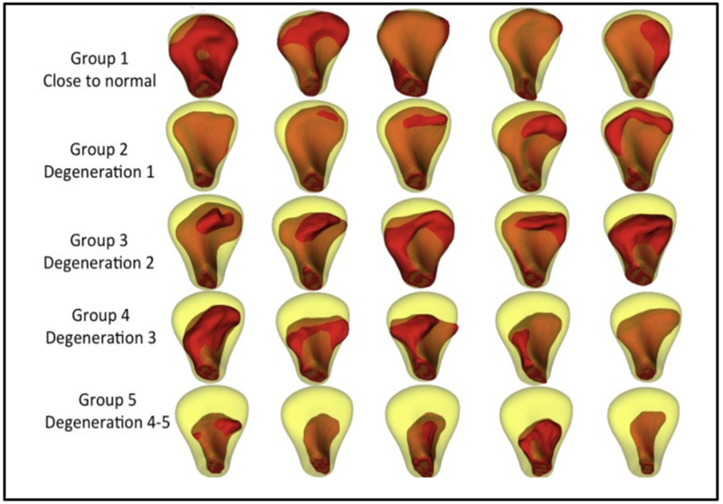
Following clinical diagnosis of TMJ osteoarthritis, a cone beam computed tomography (CBCT) scan was taken on all participants, with 0.08 mm isotropic voxel size and 4 cm × 4 cm field of view, using the 3D Accuitomo 170, Morita Corp. The study sample consists of 293 (259 training set and 34 testing set) mandibular condyle 3D surface meshes constructed from CBCT scans for the training dataset, 105 from control subjects and 154 from patients of TMJ OA. Those 3D meshes were classified in 6 groups, by consensus between 2 clinicians (MY and AR) as shown in Figure 1. Thirty-four right and left condyles from 17 patients (39.9 ± 11.7 years), who experienced signs and symptoms of the disease for less than 5 years, were included as the testing dataset.

Figure 1.

Randomly selected samples in each group, shown in red, classified by the 2 expert clinician. In yellow, the mean of the control group. G1: close to normal, G2: Degeneration 1, G3: Degeneration 2, G4: Degeneration 3 and G5: Degeneration 4 – 5.

2.2. From CBCT scan to 3D mesh

Many steps are accomplished (figure 2) before having the 3D mesh corresponding to each CBCT scan as following.

Figure 2.

Description of the 3D meshes creation from CBCT scan.

2.3. Generation of synthetic data

After the consensus between the 2 expert clinicians, the number of samples in every group is different. This problem is extremely common in machine learning. Most machine learning algorithms work better when the number of samples in every group is roughly equal. In 2002, a sampling-based algorithm called SMOTE (Synthetic Minority Over-Sampling Technique) was introduced to face imbalanced problems. This method is one of the most used thanks to its simplicity and effectiveness. The synthetic data is created by operating in “feature space” instead of “data space”. In traditional oversampling, minority class is replicated exactly. In SMOTE, new minority instances are constructed this way:

For each minority class instance c:

Neighbors = get k Nearest Neighbors (5 in our case)

n = pick randomly one of the neighbors

Creation of a new minority class r using c’s feature vector and the feature’s vector difference of n and c multiplied by a random number -> r.feats = c.feats + (c.feats - n.feats ) * rand(0,1)

2.4. Feature extraction and shape descriptors

The SVA module computes the average shape of each group of condylar dysmorphology, as well as geometric features at each vertex of the mesh and a shape descriptor, heat kernel signature. The features are stored into arrays and linked to their corresponding vertices in the 3D meshes. Those vertex-wise features are:

• Normal vector: 3 scalars for the x, y, and z coordinates

• Distances: As many components as classes

The distance to every mean group is computed.

• Curvatures: 4 scalars for mean, minimum, maximum, and Gaussian curvature.

• Shape Index: 1 scalar

The shape index and curvedness were computed using the principal curvatures (κ1, κ2) at every point in the surface. The shape index described local surface topology in terms of the principal curvatures, calculated as follows (1):

$$S=\frac{2}{\pi }\mathit{arctan}\frac{{\kappa }_1+{\kappa }_2}{{\kappa }_1-{\kappa }_2}$$ (1)

• Curvedness: 1 scalar

The curvedness was calculated as a measurement of the amount or ‘intensity’ of the surface curvature as follows (2):

$$C=\sqrt[2]{\frac{{\kappa }_1+{\kappa }_2}{2}}$$ (2)

• Position: 3 scalars for the x, y, and z coordinates.

• Heat kernel signature

The heat kernel signature (HKS) is a shape descriptor used in deformable shape analysis methods. For each point of the shape, HKS defines its feature vector representing the point’s global and local geometric features. It is based on heat kernel, fundamental solution of the heat equation. HKS uses Laplace Beltrami operator associated with the shape. Heat kernel signature should be scale invariant to deal with global and local scaling transformations. The patients of our study have different sizes of condyles depending on the gender and the age; we need to compare the 3D meshes without taking into account the scale differences. We used the heat conduction properties as shape descriptor with the heat diffusion equation as following (3):

$$\left({\Delta }_X+\frac{\partial }{\partial t}\right)u=0$$ (3)

where Δ_X is the Laplace-Beltrami operator.

Computation of the scale invariant HKS is done using heat kernel formula (solution of the heat diffusion equation [3]) in where continuous eigenfunctions and eigenvalues of the Laplace Beltrami operator are replaced by the discrete value (4):

$$K_{X,t}(x,z)={\sum }_{i=0}^{\infty }{e}^{-{\lambda }_{i}t}{\varphi }_i(x){\varphi }_i(z)$$ (4)

where λ₀, λ₁, … ≥ 0 are eigenvalues and ϕ₀, ϕ₁, … are the corresponding eigenfunctions of the Laplace-Beltrami operator, satisfying Δ_Xϕ_i = λ_iϕ_i.

The Laplace-Beltrami operator is discretized using cotangent weight scheme, defined for any function f on the mesh vertices as (5):

$${\left({\Delta }_{\widehat{X}}f\right)}_i=\frac{1}{a_i}{\sum }_j{w}_{ij}(f_i-f_j)$$ (5)

where w_ij = cot a_ij + cot b_ij for j in the 1-ring neighborhood of vertex i and zero otherwise ( a_ij and b_ij are the two angles opposite to the edge between vertices i and j in the two triangles sharing edge) and a_i are normalization coefficients proportional to the area of triangles sharing the vertex x_i.

The discrete heat kernel signature is approximated by (6):

$$h(x_l,\tau )\approx {\sum }_{l=0}^k{e}^{-{\lambda }_l{\alpha }^{\tau }}{\varphi }_{il}{}^2=\Psi e^{-T\wedge }$$ (6)

where T = diag(α^T) and $\Psi =\left({\varphi }_{il}^2\right)$

2.5. Deep neural network

Neural network architecture: The neural network learns tasks by considering examples. It is based on a collection of connected units called neurons organized in layers. We use a soft-max layer with one output per class. The output vector will be the probability for each shape to belong to a class. The algorithm extracts shape features to classify each sample in the training data in a class and can then classify new samples thanks to this probabilistic function (the soft-max function). The TensorFlow open-source library was used to train and test the neural network by constructing computational graphs. The neural network was trained to classify a given shape into one of the 6 groups indicating the severity of the disease. The input data to train the network was stored in a matrix with dimensions [number (nbr) of subjects, nbr of vertices, nbr of features]. By training a neural network we sought to identify discriminative patterns of these features and encoded them in the network (deep learning).

2.6. Comparison with machine learning algorithms

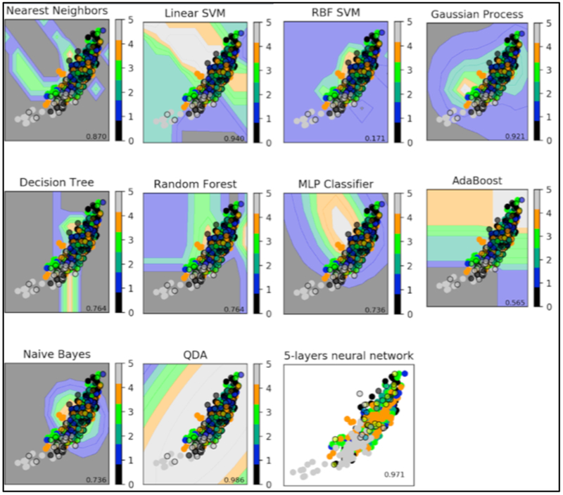
We trained and optimized nine different supervised machine learning to compare to our current deep neural network: Nearest Neighbors¹³, Linear Support Vector Machine⁹, Radial Basis Function kernel Support Vector Machine⁹, Gaussian Process¹⁰, Decision Tree¹⁴, Random Forest¹¹, AdaBoost¹⁵, Naive Bayes¹⁶ and Quadratic Discriminant Analysis¹⁷ (Figure 3).

Figure 3.

5-layers neural network compared to supervised machine learning algorithms. Supervised methods show the decision boundary in the background for the first feature. The points represent the input data with different groups (plain: training data; surrounded: testing data)

3. RESULTS

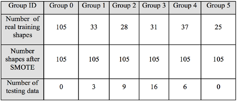
Using SMOTE algorithm creates balanced group as shown in figure 4. It allows training accuracy increasing from 86% to 92% and creates large amount of data in every group. Choosing features is decisive for the neural network to perform well. We had trained the neural network previously described with different combinations of features. We are using heat kernel signature as a shape descriptor. For each group, patterns are similar meaning a good understanding of the morphology variability (Figure 5).

Figure 4.

Number of shapes before and after SMOTE (Group 0: Control, Group 1: Close to Normal, Group 2: degeneration 1, Group 3: degeneration 2, Group 4: degeneration3, Group 5: degeneration 4-5.

Figure 5.

Shapes randomly chosen in every group with heat kernel signature plotted

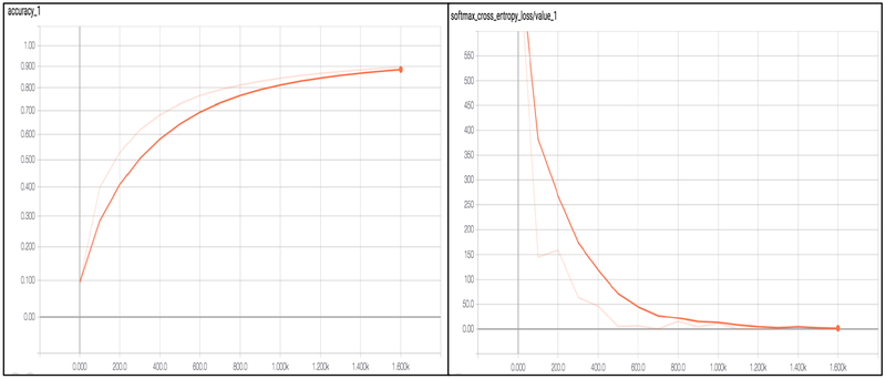
We used a neural network having 4 hidden layers with [4096, 2048, 1024, 512] neurons, a dropout layer with probability 0.5 and softmax layer with 7 outputs. The learning rate was set to 1–5. The network was trained for 100 epochs and the batch size was set to 32. The SVA training is shown in Figure 6. The maximum accuracy during training was 92%. The dataset was subdivided in two sets, training and testing in an 80/20 ratio. The testing data was not used at any point during training and it will be used to test if the trained network generalizes well for unseen data samples. After testing with 9 different machine learning algorithms, we chose the deep neural network because it’s more modulable and innovative and robust to allow addition of larger data sets as this work progresses with future collaboration with other clinical centers.

Figure 6.

Accuracy and cross entropy loss

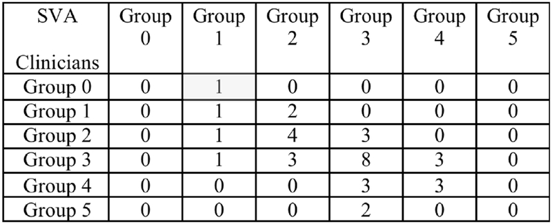
The continued enrollment of subjects to adding more data will benefit from the deep learning approach to improve the ability of the neural network to learn abstract patterns and, thus, increase the classification accuracy. Furthermore, neural networks have been shown to perform better to build a predictive tool to assess disease progression and explain variability over time. After testing with the 34 testing condyles, we obtain an accuracy of 47% of exact classification and 91% if we take an error of +/− one group as shown in Figure 7 with the confusion matrix.

Figure 7.

Confusion matrix: columns show the SVA classification of condyle morphology, rows shows the clinician expert consensus classification. The main diagonal cells are the correct classification of SVA taking as a reference the clinicians classification.

4. CONCLUSION

SVA is a novel tool to TMJ condyle analyze shape variation using deep neural networks. The results presented indicate that using shape features only favors the classification task, i.e., we do not include any information about position or orientation of the model. This classification approach seems promising, as it may help us increase our understanding about shape changes that TMJ OA patients undergo during the course of the disease. The source code repository is available at https://github.com/DCBIA-OrthoLab/ShapeVariationAnalyzer. Future work will focus on including additional predictors/features of the disease in the neural network training (e.g., clinical data, behavioral or biochemical). Clinical and behavioral data has been acquired through questionnaires, while biochemical data has been acquired through a protein analysis in saliva and plasma samples. Including these may contribute to improve the classification power of the neural network.

REFERENCES

- [1].Loeser RF, Goldring SR, Scanzello CR and Goldring MB, “Osteoarthritis: a disease of the joint as an organ.,” Arthritis Rheum. 64(6), 1697–1707 (2012). [DOI] [PMC free article] [PubMed] [Google Scholar]
- [2].Cevidanes LHS, Hajati A-K, Paniagua B, Lim PF, Walker DG, Palconet G, Nackley AG, Styner M, Ludlow JB, Zhu H and Phillips C, “Quantification of condylar resorption in temporomandibular joint osteoarthritis,” Oral Surgery, Oral Med. Oral Pathol. Oral Radiol. Endodontology 110(1), 110–117 (2010). [DOI] [PMC free article] [PubMed] [Google Scholar]
- [3].Ebrahim FH, Ruellas ACO, Paniagua B, Benavides E, Jepsen K, Wolford L, Goncalves JR and Cevidanes LHS, “Accuracy of biomarkers obtained from cone beam computed tomography in assessing the internal trabecular structure of the mandibular condyle,” Oral Surg. Oral Med. Oral Pathol. Oral Radiol. (2017). [DOI] [PMC free article] [PubMed] [Google Scholar]
- [4].Paniagua B, Ruellas AC, Benavides E, Marron S, Wolford L, Cevidanes L, Woldford L and Cevidanes L, “Validation of CBCT for the computation of textural biomarkers,” Proc. SPIE--the Int. Soc. Opt. Eng. 9417(March 2015), Gimi B and Molthen RC, Eds., 94171B (2015). [DOI] [PMC free article] [PubMed] [Google Scholar]
- [5].Gomes LR, Gomes M, Jung B, Paniagua B, Ruellas AC, Gonçalves JR, Styner MA, Wolford L and Cevidanes L, “Diagnostic index of 3D osteoarthritic changes in TMJ condylar morphology,” Proc. SPIE--the Int. Soc. Opt. Eng. 9414, Hadjiiski LM and Tourassi GD, Eds., 941405 (2015). [DOI] [PMC free article] [PubMed] [Google Scholar]
- [6].de Dumast P, Mirabel C, Cevidanes L, Ruellas A, Yatabe M, Ioshida M, Ribera NT, Michoud L, Gomes L, Huang C, Zhu H, Muniz L, Shoukri B, Paniagua B, Styner M, Pieper S, Budin F, Vimort J-B, Pascal L, et al. , “A web-based system for neural network based classification in temporomandibular joint osteoarthritis.,” Comput. Med. Imaging Graph. 67, 45–54 (2018). [DOI] [PMC free article] [PubMed] [Google Scholar]
- [7].Bronstein MM and Kokkinos I, “Scale-invariant heat kernel signatures for non-rigid shape recognition,” Proc. IEEE Comput. Soc. Conf. Comput. Vis. Pattern Recognit. (2010). [Google Scholar]
- [8].Chawla NV, Bowyer KW, Hall LO and Kegelmeyer WP, “SMOTE: Synthetic Minority Over-sampling Technique,” J. Artif. Intell. Res. 16, 321–357 (2002). [Google Scholar]
- [9].Cortes C and Vapnik V, “Support-Vector Networks,” Mach. Learn. 20(3), 273–297 (1995). [Google Scholar]
- [10].Hyun JW, Li Y, Huang C, Styner M, Lin W and Zhu H, “STGP: Spatio-temporal Gaussian process models for longitudinal neuroimaging data,” Neuroimage (2016). [DOI] [PMC free article] [PubMed] [Google Scholar]
- [11].Liaw A and Wiener M, “Classification and Regression by randomForest,” R news (2002). [Google Scholar]
- [12].Fedorov A, Beichel R, Kalpathy-Cramer J, Finet J, Fillion-Robin JC, Pujol S, Bauer C, Jennings D, Fennessy F, Sonka M, Buatti J, Aylward S, Miller JV, Pieper S and Kikinis R, “3D Sheer as an image computing platform for the Quantitative Imaging Network,” Magn. Reson. Imaging (2012). [DOI] [PMC free article] [PubMed] [Google Scholar]
- [13].Keller JM and Gray MR, “A Fuzzy K-Nearest Neighbor Algorithm,” IEEE Trans. Syst. Man Cybern (1985). [Google Scholar]
- [14].Kohavi R, “Scaling Up the Accuracy of Naive-Bayes Classifiers: a Decision-Tree Hybrid,” Proc. 2nd Int. Conf. Knowl. Discov. Data Min (1996). [Google Scholar]
- [15].Rätsch G, Onoda T and Müller KR, “Soft margins for AdaBoost,” Mach. Learn (2001). [Google Scholar]
- [16].Vikramkumar B, V. and Trilochan., “Bayes and Naive Bayes Classifier,” arXiv (2014). [Google Scholar]
- [17].Srivastava S, Gupta M and Frigyik B, “Bayesian Quadratic Discriminant Analysis,” J. Mach. Learn. Res. (2007). [Google Scholar]