Diagnostic tests: how to estimate the positive predictive value

Abstract

When a patient receives a positive test result from a diagnostic test they assume they have the disease. However, the positive predictive value (PPV), ie the probability that they have the disease given a positive test result, is rarely equal to one. To assist their patients, doctors must explain the chance that they do in fact have the disease. However, physicians frequently miscalculate the PPV as the sensitivity and/or misinterpret the PPV, which results in increased anxiety in patients and generates unnecessary tests and consultations. The reasons for this miscalculation as well as three ways to calculate the PPV are reviewed here.

Prevalence of glioma is 0.003%. A patient comes into the clinic complaining of headaches and memory loss. A new blood test for diagnosis of glioma is available. The patient tests positive. From the literature (see Table 1) you know that the sensitivity of the test is 96.7% and the false positive rate is 4%. What is the probability that this patient who tested positive actually has glioma?

This is an understandably difficult problem, since it pertains to conditional probabilities (sensitivity, specificity, and positive predictive value [PPV]) and varying reference populations (those with disease and those without). Nonetheless, an informed interpretation of diagnostic tests is increasingly important, especially as novel biomarkers are used in the detection of disease. Unfortunately, studies have shown that more than 75% of the doctors answer questions similar to that above incorrectly.^1–5

Table 1.

Fictional table from literature.

	Disease Status		Total
	Glioma Present	Glioma Absent
Test Result
Positive	29	2	31
Negative	1	48	49
Total	30	50	80

In this data, the prevalence of disease is P(D) = 30/80 = 0.375; the sensitivity is P(Test positive | Glioma present) = 29/30 = 0.967; the false positive rate is P(Test positive | Glioma absent) = 2/50 = 0.04. See Table 2 for formulas.

The goal of this review is to ease the calculation of conditional probabilities (eg, the PPV in the example above) by explaining three ways to solve them: conditional probability equations, tree diagrams (with probabilities), and natural frequencies. You have the option of reviewing all three or just one or two of the approaches. Any of the three will get you to the correct answer. We begin with the calculation via conditional probabilities and follow with building tree diagrams for a visual representation. Subsequently, we illustrate a way to translate this information via natural frequencies for you and your patients so that they too understand the meaning of a positive or negative test result.

Approach 1: Conditional Probability Equations

Conditional probabilities are important in the interpretation of diagnostic tests because the test results influence our understanding of whether the patient has a disease. However, the test results are not synonymous with the presence or absence of disease. The conditional probabilities that we need to understand are sensitivity, specificity, PPV, and negative predictive value (NPV). These probabilities are defined by two events: the presence of disease and a positive test result.

Sensitivity is defined as the probability of a positive test result given the presence of disease, written as: P(positive test | disease present). The vertical line can be read as “given.” Specificity is defined as the probability of a negative test result given absence of disease, ie $P(\text{negative}\text{test | disease}\text{absent})$.PPV is defined as the probability of the presence of disease given a positive test result, ie, $P(\text{disease present | positive}\text{test})$.NPV is defined as the probability of the absence of disease given a negative test result, ie, $P(\text{disease}\text{absent | negative}\text{test})$. Given the similarities in calculation between PPV and NPV we will only focus on the former here.

There are two important things to know about conditional probabilities. First, conditional probabilities are not reciprocal, ie,

$$P(\mathrm{Event}A|\text{Event}B)\ne P(\mathrm{Event}B|\text{Event}A).$$

This is important to note as this means that sensitivity does not equal PPV, ie

$$P(\mathrm{positive}\text{test}|\mathrm{diseasepresent})\ne P(\text{disease present }|\text{positive}\text{test}).$$

This is one of the most common errors that doctors make when calculating PPV – they simply equate it with the test's sensitivity.

Second, you can write a conditional probability as:

$$P(\mathrm{Event}A|\mathrm{Event}B)=\frac{P(\text{Event}A\mathbf{a}\mathbf{n}\mathbf{d}\text{Event}B)}{P(\text{Event}B)}.$$

The importance of the fraction on the right has to do with how we will connect the sensitivity to PPV and will become clearer when we learn how to rewrite the numerator on the right-hand side. To do so, we need the multiplication rule, which is the probability that both events occur, ie $P(\text{Event}A\mathbf{a}\mathbf{n}\mathbf{d}\text{Event}B)$. This can be written as:

$$P(\text{Event}A\mathbf{a}\mathbf{n}\mathbf{d}\text{Event}B)=P(\text{Event}B)\ast P(\text{Event}A|\text{Event}B)$$

or with our events as:

$$P(\text{disease present}\text{and positive}\text{test})=P(\text{disease present})\ast P(\text{positive}\text{test;|;disease present})$$

which is equivalent to:

$$P(\text{True positive})=\text{Prevalence}\ast \text{Sensitivity}.$$

Similarly the probability of a false positive can be written as:

$$\begin{array}{ll}& P(\text{False positive})\\ & =P(\text{disease}\text{absent}\text{and positive}\text{test})\\ & =P(\text{disease}\text{absent})\ast P(\text{positive}\text{test |;disease}\text{absent})\\ & =(1-\text{Prevalence)}\ast \text{False}\text{Positive}\text{Rate}\end{array}$$

Now we can connect the PPV to the sensitivity:

$$\text{PPV}=P(\text{disease present |}\text{positive}\text{test})$$

Expressed as the other form of conditional probability, we can see this as:

$$=\frac{P(\text{disease present}\mathbf{a}\mathbf{n}\mathbf{d}\mathbf{p}\mathbf{o}\mathbf{s}\mathbf{i}\mathbf{t}\mathbf{i}\mathbf{v}\mathbf{e}\text{test})}{P(\text{positive}\text{test})}$$

And by applying the multiplication rule, we can rewrite this as:

$$\begin{array}{ll}=& \frac{P(\text{disease present})\ast P(\text{positive}\text{test | disease present})}{P(\text{positive}\text{test})}\\ =& \frac{\text{Prevalence}\ast \text{Sensitivity}}{P(\text{positive}\text{test})}\end{array}$$

In the denominator, a positive test can come from those patients with the presence of disease (true positives) and those with the absence of disease (false positives). Therefore we can write: $P(\text{positive}\text{test})=P(\text{true positive})+P(\text{false positive}).$ The two probabilities on the right were defined above. We can continue the calculation to get the PPV:

$$=\frac{\text{Prevalence}\ast \text{Sensitivity}}{P(\text{true positive})+P(\text{false positive})}$$

In the example of the test for glioma above, we would substitute the values for prevalence, sensitivity, and false positives, and calculate:

$$=\frac{(0.00003)\ast (0.967)}{((0.00003)\ast (0.967))+((1-0.00003)\ast (0.04))}=0.000725$$

Thus, the chance that the patient has glioma given a positive test result is 0.07%.

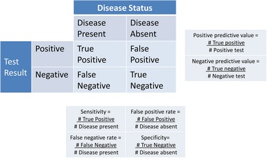
There are many similarities between a 2 × 2 table (Table 1) and conditional probabilities. You can see from Table 2 how to calculate sensitivity, specificity, and PPV from a 2 × 2 table. However, PPV can only be calculated from a 2 × 2 table if the prevalence [P(Disease present) = number of people with disease/number of people in population (or sample)] in the table is the same as that in the population. Typically the reason the prevalence in a 2 × 2 table does not reflect the population prevalence is because the table is based on case-control data in which a specified number of cases (patients with disease) and controls (patients without disease) are studied for the purpose of finding associations. For example, in Table 1 the hypothetical data are based on a case-control study with 30 cases and 50 controls and thus the prevalence of disease is $(30/80)=37.5\mathrm{\%}.$ Using the same calculations as above but with a prevalence of 37.5%, the PPV equals 94%, which is incorrect, as we know the prevalence in the population is 0.003%. Thus, if the prevalence of the disease in a 2 × 2 table is not the same as in the population you cannot calculate the PPV (or NPV).

Table 2.

A 2 × 2 table with test results in the rows and disease status in the columns

Sensitivity, Specificity, and False positive/negative rate can be calculated from any such 2 × 2 table. Positive and Negative predictive values can only be calculated from a 2 × 2 table if the prevalence of disease in the table is the same as that in the population. It should be noted that the false positive rate is the P(negative test | disease absent) while the false positive in the 2 × 2 table is the P(positive test and disease absent).

Approach 2: Tree Diagrams

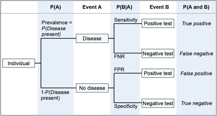
Another way to display the data is in a tree diagram^3,6 (Fig. 1). Starting on the left at the “Individual” the first split corresponds to disease status, the patient either has disease or does not. The top line going from “Individual” to “Disease” shows the prevalence of disease while the bottom line shows the probability of not having the disease, $1-\text{Prevalence}$. Similar to disease status, the test result can either be positive or negative. The line between “Disease” and “Positive test” displays the sensitivity, ie $P(\text{positive}\text{test | disease present})$, whereas the line between “No Disease” and “Negative test” shows the specificity, ie $P(\text{negative}\text{test | disease}\text{absent})$. The conditional probabilities associated with the other two lines, the false positive/negative rates, can be written similarly. Note that the two lines coming from the same box must sum to one, eg $\text{prevalence}+$$(1-\text{prevalence})=1$. That is also true for sensitivity and the false negative rate as well as the false positive rate and specificity. The four squares of the 2 × 2 table can also be calculated on the far right of the tree diagram by using the multiplication rule, eg

$$\begin{array}{ll}& P(\text{true positive})\\ & =P(\text{disease present}\text{and positive}\text{test})\\ & =P(\text{disease present})\ast P(\text{positive}\text{test | disease present})\\ & =\text{Prevalence}\ast \text{Sensitivity}\end{array}$$

$$\begin{array}{ll}& P(\text{false positive})\\ & =P(\text{disease}\text{absent}\text{and positive test})\\ & =P(\text{disease absent})\ast P(\text{positive test | disease absent)}\\ & =(1-\text{Prevalence})\ast \text{False positive rate}.\end{array}$$

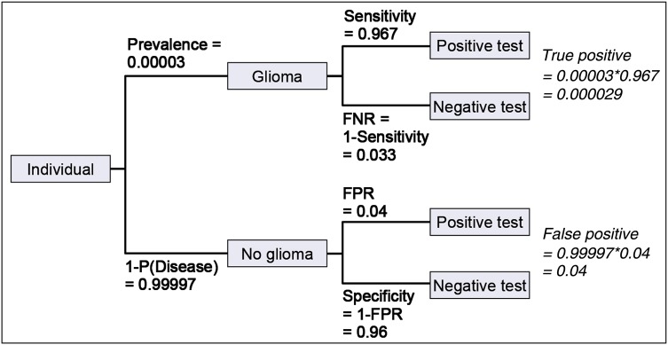
We can display the information from the original question in a tree diagram to help calculate the PPV. In Fig. 2, the known information is in bold and the inferred information is in italic. Note that the people with a positive test are either true positives (disease present and a positive test) or false positives (no disease and a positive test). Because the prevalence in the tree diagram is considered in calculating true positives a simpler way of calculating the PPV is:

$$\text{PPV}=P(\mathrm{Disease}|\text{Positive}\text{test})$$

Fig. 1.

Tree diagram representing all possible outcomes of a diagnostic test. P(A) is the probability of Event A. P(B|A) is the conditional probability of Event B given Event A. FPR is the false positive rate = P(Positive test | Disease absent). FNR is the False negative rate = P(Negative test | Disease present).

Fig. 2.

Tree diagram representing all possible outcomes and condition probabilities given in hypothetical diagnostic test example. Text in bold is given in example. Text in italic is calculated from given information in bold. FPR is the false positive rate = P(Positive test | Disease absent). FNR is the False negative rate = P(Negative test | Disease present).

Or, as expressed as the other form of conditional probability:

$$\begin{array}{ll}=& \frac{P(\text{Disease}\text{and}\text{Positive}\text{test})}{P(\text{Positive}\text{test})}\\ =& \frac{P(\text{True}\text{Positive})}{P(\text{True}\text{Positive})+P(\text{False}\text{Positive})}\end{array}$$

If we substitute numbers from the tree diagram, we can calculate:

$$=\frac{(0.000029)}{(0.000029)+(0.04)}=0.000725$$

Thus, the chance that the patient has glioma given a positive test result is 0.07%. This PPV should be clearly communicated to the patient. As it can be difficult to explain conditional probabilities to patients, we will explore an alternative option.

Approach 3: Natural frequencies

To help patients understand conditional probabilities you can translate them to natural frequencies with or without the use of a tree diagram.^1,3 Natural frequencies are the way most people are presented with statistics and, thus, make interpretation simpler. We can directly translate the original question into natural frequencies and illustrate the ease with which the question can be answered.

Three out of every 100 000 people have glioma. A patient comes into the clinic complaining of headaches and memory loss. A new blood test for diagnosis of glioma is available. She tests positive. From the literature you know that of the three people out of 100 000 with glioma, all three will likely have a positive blood test. Of the 99 997 people without glioma, 4000 will still have a positive blood test. Of the patients with a positive blood test, how many actually have glioma?

Now the answer is much more straightforward to calculate: it is $3/(3+4000)=\mathrm{0.0007.}$ Again, this is the PPV, the chance that a patient with a positive test result actually has glioma.

One of the reasons natural frequencies make this problem easier to understand is that they use the same reference group. For example, three patients (with a positive blood test and glioma) and 4000 patients (with a positive blood test and no glioma) both refer to the same group of 100 000 people. In contrast, in the original question the sensitivity refers to the group of three patients with glioma while the specificity refers to the group of 4000 patients without glioma. A pitfall of using natural frequencies is that mistakes can be made in translating the conditional probabilities to frequencies and thus caution must be used.

Conclusion

Positive predictive value is the probability that a person who receives a positive test result actually has the disease. This is what patients want to know. Nonetheless, physicians frequently miscalculate and/or misinterpret the PPV, which results in increased anxiety in patients and generates unnecessary tests and consultations. One of the reasons for miscalculation is that conditional probabilities are not reciprocal, meaning that the $P(B|A)\ne P(A|B)$, or in our example that sensitivity does not equal PPV. A second reason is that the PPV relies on the prevalence of disease and therefore the PPV cannot be calculated from a data set that does not have the same prevalence as the population. Finally, conditional probabilities can be conceptual and many studies have shown that reframing the problem in natural frequencies (with or without tree diagrams) increases the ability of a physician to correctly calculate the PPV.^1,3

Here we have shown three ways to calculate the PPV: conditional probabilities, tree diagrams and natural frequencies. In all three, we show that the PPV of the hypothetical blood test equals 0.07%. The implication of this is crucial but often goes unnoticed. For any rare disease, such as glioma, the percent of false positives tends to be appreciable even though the sensitivity and specificity may be high. The ramification is that the vast majority of positive test results will be false positives. An advantage of a low prevalence of disease is that a patient with a negative test result is very unlikely to have the disease, ie the negative predictive value (NPV) is large. In the hypothetical example the NPV can be calculated similarly to the PPV and shown to equal 99.99%.

Given the current focus on finding novel biomarkers to be used in the detection of disease, an informed interpretation of diagnostic tests is increasingly important. Equally important is the translation of this information to your patients. We hope these tools will be helpful in both understanding and relaying conditional probabilities to your patients.

Funding

This study was supported by R01 CA163687 (Annette M. Molinaro, Principal Investigator).

References

- 1. Gigerenzer G, Edwards A. Simple tools for understanding risks: from innumeracy to insight. Br Med J. 2003-09-25 21:58:31, 2003;327(7417):741–744. [DOI] [PMC free article] [PubMed] [Google Scholar]
- 2. Casscells W, Schoenberger A, Graboys TB. Interpretation by Physicians of Clinical Laboratory Results. N Engl J Med. 1978;299(18):999–1001. [DOI] [PubMed] [Google Scholar]
- 3. Friederichs H, Ligges S, Weissenstein A. Using Tree Diagrams without Numerical Values in Addition to Relative Numbers Improves Students’ Numeracy Skills: A Randomized Study in Medical Education. Med Decis Making. 2014;34(2):253–257. [DOI] [PubMed] [Google Scholar]
- 4. Manrai AK, Bhatia G, Strymish J, Kohane IS, Jain SH. Medicine's uncomfortable relationship with math: Calculating positive predictive value. JAMA Intern Med. 2014;174(6):991–993. [DOI] [PMC free article] [PubMed] [Google Scholar]
- 5. Eddy D. Probabilistic reasoning in clinical medicine: problems and opportunities. In: Kahneman D, Sloviv P, Tversky A, eds. Judgement under uncertainty: Heuristics and Biases. Cambridge, UK: Cambridge University Press; 1982:249–267. [Google Scholar]
- 6. Baldi B, Moore DS. The Practice of Statistics in the Life Sciences, 2nd ed. New York, NY: W. H. Freeman; 2010. [Google Scholar]