Predicting the Unpredictable: Weighted Averaging of Past Stimulus Timing Facilitates Ocular Pursuit of Randomly Timed Stimuli

Abstract

In motor control, prediction of future events is vital for overcoming sensory-motor processing delays and facilitating rapid and accurate responses in a dynamic environment. In human ocular pursuit this is so pervasive that prediction of future target motion cannot easily be eliminated by randomizing stimulus parameters. We investigated the prediction of temporally randomized events during pursuit of alternating constant-velocity (ramp) stimuli in which the timing of direction changes varied unpredictably over a given range. Responses were not reactive; instead, smooth eye velocity began to decelerate in anticipation of each target reversal. In the first experiment, using a continuous-motion stimulus, we found that the time at which this occurred was relatively constant regardless of ramp duration, but increased as mean ramp duration of the range increased. Regression analysis revealed a quantitative association between deceleration timing and the previous two or three ramp durations in a trial, suggesting that recent stimulus history was used to create a running average of anticipatory timing. In the second experiment, we used discrete motion stimuli, with intervening periods of fixation, which allowed both target velocity and reversal timing to be varied, thereby decoupling ramp duration and displacement. This enabled us to confirm that the timing of anticipatory deceleration was based on the history of timing, rather than displacement, within the stimulus. We conclude that this strategy is used to minimize error amid temporal uncertainty, while simultaneously overcoming inherent delays in visuomotor processing.

Introduction

Prediction is a common and pervasive feature of motor control, necessary to overcome the sensory-motor processing delays that would otherwise hinder timely and accurate responses to events in an animal's constantly changing environment. For example, it takes the human oculomotor system ∼100 ms to respond to an unexpected change of direction in a discretely moving target (Robinson et al., 1986; Carl and Gellman, 1987). If target motion is periodic, however, the eye often begins to reverse in advance of target reversal after only one or two cycles (Dodge et al., 1930), thereby overcoming this inherent visuomotor processing delay.

It has often been assumed (Stark et al., 1962; Dallos and Jones, 1963; Bahill et al., 1980) that a reactive mode of responding persists as long as target motion remains aperiodic. This view was challenged, however, by Kowler and Steinman (1979a,b, 1981) who demonstrated the ubiquitous nature of anticipatory behavior and its influence on very low velocity (<1°/s) smooth eye movements. They concluded that subjects always try to predict future target motion, regardless of the nature of the stimulus. Several studies have confirmed this, using higher velocity stimuli more representative of the velocities attained during active smooth pursuit tracking. For example, it is known that anticipatory smooth movements, occurring before target onset, cannot be abolished by randomizing stimulus parameters (Heinen et al., 2005); furthermore, smooth eye velocity begins to decelerate toward the end of ramps of randomized duration (Krauzlis and Miles, 1996; Barnes et al., 2005).

This prediction of randomly timed events is known to be influenced by the history of stimulus (and under some circumstances, response) characteristics. For example, history effects are known to influence both the latency (Heinen et al., 2005; Badler and Heinen, 2006) and velocity (Kowler et al., 1984; Kowler, 1989) of anticipatory smooth pursuit, suggesting that in unpredictable circumstances the probability of what the stimulus will do next is calculated on the basis of what has occurred in the recent past. However, prediction is also influenced in these circumstances by the generation of cognitive expectations that can override history effects, for example, if information about forthcoming stimulus motion is provided in the form of a visual or auditory cue (Kowler, 1989).

The aim of this study was to investigate and quantify the mechanism underlying the prediction of randomly timed events by the ocular-motor system. We used alternating constant-velocity stimuli, presented either as discrete pairs of ramps or as a continuous irregular waveform; ramp duration was randomized over a given range. As expected, eye velocity generally began to decelerate before target reversal. The time at which this occurred was relatively constant regardless of ramp duration, but increased as mean ramp duration for the range increased. Regression analyses revealed a quantitative association between deceleration timing and recent ramp durations. We conclude that, when stimulus timing is random, a running average of anticipatory response timing is created, based on stimulus timing history, and used to initiate pursuit deceleration before target reversal.

Materials and Methods

All experiments were conducted in accordance with the Declaration of Helsinki and with the approval of the local ethics committee. Human subjects took part after giving voluntary, informed consent; they had no known neurological or oculomotor problems and had normal or corrected-to-normal vision. Both authors participated in the experiments; all other subjects were naive to the purpose of the experiments.

Apparatus

Subjects sat in a darkened room and were presented with a red target against a blank background. The target comprised a ring of dots subtending 1.2° at the eye; it was formed by optically reducing and projecting onto a screen (2.5 m wide × 1.5 m high) 12 ultrabright light-emitting diodes that could be switched on and off very rapidly (rise time, ∼5 μs). The screen was located 1.5 m from the subject's head. The target image was moved in the horizontal axis by a servo-controlled mirror; its motion was controlled by a computer-generated waveform. The head was immobilized by side clamps and a chin rest. Eye movements were recorded by a limbus tracking device (Skalar Iris) that was firmly attached to the head.

Experiment 1

The aim of experiment 1 was to determine whether subjects would anticipate target direction changes in a continuous-motion stimulus in which target reversal timing was randomized within a certain range.

Subjects.

Nine subjects (five females) participated; their mean age was 31.2 years (SD, 12.3). Four subjects had previous experience of oculomotor experiments.

Procedure.

The target moved at constant velocity (15°/s) in an irregular triangular waveform (i.e., the time at which the target changed direction varied) (see Fig. 1A,B). Each trial effectively comprised 32 consecutive ramps, alternating in direction and varying in duration. Eight different ramp durations (RDs) were presented four times each within a trial (hence 32 in total). RD order was randomized, the only constraint being that the same RD was never presented consecutively. Three RD ranges were constructed, in which RD increased from the range minimum (min) to the range maximum (max) in increments of 60 ms: SHORT range: min RD, 420 ms; max RD, 840 ms (mean RD, 630 ms; mean displacement, 9.5°); MED range: min RD, 600 ms; max RD, 1020 ms (mean RD, 810 ms; mean displacement, 12.2°); LONG range: min RD, 780 ms; max RD, 1200 ms (mean RD, 990 ms; mean displacement, 14.9°). Each subject performed three trials (with different randomization) of each RD range, yielding 12 repeats of each RD in each range. They were informed that the timing of target reversals would be unpredictable and were simply instructed to follow the target as closely as possible.

Figure 1.

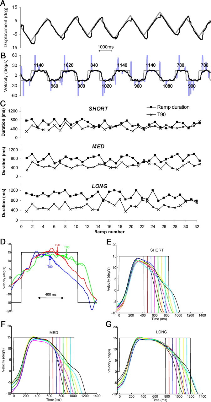
A, B, An example of eye (black trace) and target (gray trace) displacement (A) and eye and target velocity (B) for subject 6 in experiment 1. In the velocity trace, saccades are shown in blue; black numbers denote RD in milliseconds. C, T₉₀ and ramp duration data for subject 9. An example trial is shown for each range (top, SHORT; middle, MED; bottom, LONG). D shows how a quadratic smoothing function (dotted lines) was used to determine average peak eye velocity and the derivation of the time (T₉₀; filled circles) at which eye velocity first fell below 90% of peak velocity. Three example responses are shown from an individual subject in response to RD = 900 ms in the MED condition. E–G, Mean smooth eye velocity profiles, averaged over all subjects (n = 9) and all responses for each RD in the SHORT (E), MED (F), and LONG (G) ranges, respectively.

In a subset of experiment 1, subjects 3 and 6 plus four additional subjects (who did not participate in the main experiment) repeated this task and also performed an additional condition in which ramp duration was blocked, rendering stimulus timing predictable. In this predictable condition (PRD), RD ranged from 420 to 1200 ms in increments of 60 ms as in the random (RND) condition, but each RD was repeated 14 times within a block. Successive blocks were separated by several seconds in which the screen was blank; RD was randomized between blocks.

Experiment 2

Since target velocity was constant in experiment 1, it was not possible to determine whether timing of anticipatory pursuit deceleration was based on stimulus timing or stimulus displacement. The aim of experiment 2, therefore, was to discriminate between these factors by varying target velocity as well as duration in the RND condition, thereby uncoupling the relationship between ramp timing and ramp displacement. To accomplish this with a continuous-motion stimulus would be difficult because changing both velocity and timing at each reversal would change expectations about both. It is known, for example, that the anticipatory response that occurs before an abrupt change in direction is influenced by expected velocity after the change (Boman and Hotson, 1992; Barnes and Schmid, 2002). To avoid any possibility of such an influence, we adopted a technique in which stimuli were presented as discrete double ramps with identical speed before and after reversal of direction.

Subjects.

Seven subjects (three females) performed the “single-velocity” condition; their mean age was 32.6 years (SD, 13.0). Five had experience of oculomotor experiments. Six subjects (three females) performed the “multiple-velocity” condition; their mean age was 40.2 years (SD, 11.9). All had experience of oculomotor experiments.

Procedure.

Each trial comprised a series of double-ramp stimuli that started from 20° left of center and moved rightward before returning leftward at the same speed. This method allowed both the speed and duration of each ramp pair to be randomized while maintaining the property of identical speed before and after reversal, as in experiment 1. Note that the objective was to determine the time at which eye deceleration was initiated in relation to the onset and reversal of the first ramp; the role of the second (leftward) ramp therefore was simply to create this target direction reversal. Within each trial, 32 such rightward and leftward ramp pairs were presented. The time between the end of the leftward ramp of one pair and the beginning of the rightward ramp of the next pair varied randomly between 700 and 2300 ms. An audio warning cue (80 ms duration) occurred 400 ms before each rightward ramp. Within each pair, ramp speed and duration remained constant but for different ramp pairs either one or both of these parameters could be varied. There were three ranges, SHORT, MED, and LONG, with RDs identical to the corresponding conditions in experiment 1. The single-velocity condition was used to establish whether similar stimulus history effects would be observed with this discrete ramp stimulus to those seen with the continuous ramp stimuli of experiment 1. In the single-velocity condition, the eight different RDs were randomized, but target velocity remained constant at 30°/s. Each subject performed two trials of this condition for each range. In the multiple-velocity condition, the eight different RDs were combined with four different target velocities (18, 22, 26, and 30°/s). Note that simple multiples of velocity were avoided to increase the number of displacement and timing combinations. Each RD and velocity combination was presented once; hence there were 32 ramp pairs in total. The order of presentation of the RD/velocity combinations was randomized. Each subject performed two trials of the multiple-velocity condition for each range. For both single- and multiple-velocity conditions, subjects were aware that the timing of target reversals would be unpredictable and were simply instructed to follow the target as closely as possible.

Data analysis

Recorded data were low-pass filtered at 80 Hz and sampled every 4 ms (i.e., 250 Hz). Eye and target velocity were derived from the digitized data by the two-point central difference method and saccades were removed from the eye velocity signal using a technique described in detail previously (Bennett and Barnes, 2003). Linear interpolation was used to fill the gaps left by the saccades removed (for justification of using this technique, see Collins and Barnes, 2006), and the resultant data were then further filtered using a zero-phase autoregressive low-pass digital filter with a cutoff frequency of 30 Hz.

The time at which the eye velocity response to a particular ramp began to decelerate before reversing direction was defined as the time (T₉₀) at which smooth eye velocity fell below 90% of its average peak level (V_pk). Responses to a particular RD could vary widely in dynamic characteristics, as shown by the three examples in Figure 1D and usually exhibited oscillations of velocity. To avoid such oscillatory fluctuations being mistaken for anticipatory decline, V_pk was calculated after averaging eye velocity using a quadratic function to smooth the trace in the region of peak velocity (see Fig. 1D). The function was applied to a region starting at the first point after target onset at which eye velocity exceeded 75% of peak eye velocity and ending when eye velocity then subsequently fell below 50% of its peak. This satisfactorily encompassed both the region around peak velocity and the initial portion of response decay. D₉₀ was defined as target displacement at the time that T₉₀ was attained. In the PRD condition of experiment 1, mean T₉₀ for each RD was attained by averaging T₉₀ in response to presentations 3–14 within a block. To check the validity of using a smoothing function to derive the time of eye deceleration, an additional method was used for experiment 1, in which the time (T₈₀) at which smooth eye velocity first fell below 80% of its actual peak velocity was calculated. The results obtained by the two methods were not qualitatively different, as illustrated in Figure 2D. As additional performance indicators, eye velocity at the end of each ramp (V_END) and average eye deceleration between T₉₀ and ramp end (A_END) were also calculated.

Figure 2.

Average T₉₀ values for individual subjects (subjects 2, 5, and 8 in A–C, respectively) and averaged across all nine subjects (D) for experiment 1. In A–C, each data point represents mean T₉₀ (+1 intrasubject SE) averaged across the four instances of each RD in each trial and the three trial repeats for each range (SHORT, MED, and LONG). In D, each data point represents these same values averaged across all subjects (+1 intersubject SE); gray traces show T₈₀ values, calculated as described in Materials and Methods. For the two RDs that were present in all three ranges (780 and 840 ms), T₉₀ increased significantly from SHORT to MED (paired t tests; RD = 780 ms: t = 4.9, p = 3.1 × 10⁻⁶, RD = 840 ms: t = 4.6, p = 1.3 × 10⁻⁵) and from MED to LONG (RD = 780 ms: t = 6.3, p = 7.4 × 10⁻⁹; RD = 840 ms: t = 6.1, p = 1.4 × 10⁻⁸). The dotted line in all graphs represents the time at which the target reversed direction for each RD.

The influence on T₉₀ of the recent history of both the stimulus and the response in experiment 1 was analyzed using a method which was based on the “node” or “tree” method of assessing sequential effects (Falmagne et al., 1975; Kowler, 1989) and adapted by Badler and Heinen (2006) to accommodate paradigms that do not involve an “either/or” mode of responding. T₉₀ values for each subject in each RD range were categorized as “LOWER” if they fell within the lower 30th percentile of the response distribution and “UPPER” if they fell within the upper 30th percentile of the distribution. The influence of preceding UPPER or LOWER responses was then assessed by averaging T₉₀ values according to the classification of the preceding response. A similar analysis was performed to assess the effect of preceding UPPER and LOWER stimuli—RDs within each range were classified in the same way, and average T₉₀ values were then calculated depending on the classification of preceding RDs. In both experiments, the effect on T₉₀ of the current stimulus (ramp “n”) and up to eight previous stimuli (i.e., n − 1, n − 2 … n − 8) was assessed in a more detailed manner using multiple regression analyses. Note that in experiment 1, ramp n − 1 denoted the previous ramp in the trial, which always moved in the opposite direction to the current one. In experiment 2, however, ramps were presented in pairs, but the purpose of the second ramp of the pair was simply to produce a target direction reversal; therefore, the relevant previous ramp for comparison (i.e., ramp n − 1) was the first ramp of the previous pair, which was in the same direction as the current one.

Statistical analyses were performed using SPSS software. All data were tested for departures from normality using the Shapiro–Wilk statistic but no transformation of the data was deemed necessary to perform parametric tests. Comparisons within the data were made using either paired t tests or repeated-measures ANOVA. Before performing an ANOVA, the data were tested for sphericity using the Mauchly test. This test examines the covariance matrix for symmetry (i.e., within the matrix, variances should be equal and covariances should equal zero). If the Mauchly test showed that the data were not spherical, then a Greenhouse–Geisser correction was used to calculate adjusted p values in the subsequent ANOVA.

Results

Experiment 1

In the main task of experiment 1, subjects tracked a target that moved at constant velocity (15°/s) in an irregular triangular waveform [i.e., the duration of each successive ramp component varied unpredictably over a given range of durations (SHORT, MED, or LONG)]. An example of the response of an individual subject (subject 6) to the stimulus is shown in Figure 1. This subject's responses were typical, in that it is evident from the eye displacement trace (Fig. 1A) that there was considerable variability in the response to changes in target direction. In some instances, eye displacement continued in the same direction for several hundred milliseconds after the target had reversed direction, whereas in others the eye reversed direction at about the same time as the target.

This subject's eye velocity, however, normally began to decrease well before the target reversed direction (Fig. 1B), even though target reversal timing was randomized. This is also apparent from the mean smooth eye velocity profiles (Fig. 1E–G), which show data averaged over all subjects and all responses for each RD in each range. It is clear that within each range the decay of the response from peak velocity was very similar for all RDs, with very little divergence between average responses until at least 50 ms after the reversal time of the shortest RD for that range. Changes in velocity were thus anticipatory of target turnaround and were not a reactive, visual feedback-driven response to the randomly timed changes in target direction. This anticipation is reflected in the T₉₀ data, which show, for the response to each individual ramp, the time at which the eye decelerated to <90% of its peak in preparation for reversing direction. Figure 1D shows how T₉₀ was defined in three example responses. Figure 1C shows, for subject 9, how T₉₀ varied throughout individual trials—an example trial is presented for each RD range. It is clear that, for almost all responses, T₉₀ was less than the corresponding ramp duration for each of the 32 ramps within a trial.

For each range, absolute T₉₀ values varied between subjects, but the pattern of response between ranges was very similar for all subjects (Fig. 2). Average T₉₀ was much lower than RD (denoted by the dotted lines in Fig. 2), confirming that, on average, eye velocity began to decelerate well before target direction reversed. Furthermore, there was no apparent relationship between T₉₀ and RD: mean T₉₀ remained fairly constant as RD increased within each range. As RD increased across ranges from SHORT to MED to LONG, however, there was a corresponding increase in average T₉₀—mean values were 465, 537, and 634 ms for the SHORT, MED, and LONG ranges, respectively. Two-way ANOVA, with range and RD as factors, confirmed that there was a significant increase in T₉₀ with range (F_(2,16) = 93.53; p = 3.6 × 10⁻⁶), but no significant change with RD (F_(7,56) = 1.82; p = 0.18). These results imply that the response to an individual RD was not influenced by the RD itself but was dependent on the overall range of RDs within which that RD was presented in a trial.

Associated with the changes in mean T₉₀, there were consistent changes in the distribution of T₉₀ values for SHORT, MED, and LONG ranges. This is apparent from the T₉₀ frequency histograms (Fig. 3A), obtained by pooling data from all nine subjects for each range. There was a marked shift to the right (i.e., an increase in T₉₀) as RD increased across ranges. It is also apparent that histogram peak varied with range, modal bin values were 460, 580, and 640 ms for the SHORT, MED, and LONG ranges, respectively. There was also a concomitant increase in the width of the histograms from SHORT to MED to LONG, indicating increasing variability of the T₉₀ distributions. It is well established that, when judgments are made regarding the duration of a time interval, the SD of perceived duration increases with interval duration, a concept known as the scalar property (Gibbon, 1977). One consequence of the scalar property is the superimposition of frequency histograms when plotted on a normalized scale (Church and Gibbon, 1982). To determine whether our data from the three different RD ranges conformed to the scalar principle, pooled T₉₀ data for each range were normalized by dividing each value by the mean of the pooled data. The peaks and widths of the resulting histograms (Fig. 3B) were very similar for the three ranges, showing that normalization of the data had indeed led to the superimposition of the histograms. This confirms that the data adhered to the scalar principle and suggests that the pursuit response was controlled by a system that included an active time estimation mechanism, despite stimulus timing being randomized within each range. The T₉₀ data in Figure 2 showed that response timing was not related to the current RD in the stimulus because as RD increased within each range there was no corresponding increase in T₉₀. This was confirmed by plotting, within each range, separate T₉₀ frequency histograms for the response to each RD. Data from the LONG range are presented in Figure 3C; similar results were obtained for the SHORT and MED ranges. The peaks and widths of the histograms were very similar and there was no systematic shift to the right as RD increased (i.e., the non-normalized histograms were approximately superimposed). Normalizing the data (Fig. 3D), therefore, had very little effect on the frequency distributions.

Figure 3.

Frequency histograms for T₉₀ data (pooled from all subjects) from experiment 1. In A and B, data are pooled across all RDs within each of the three ranges; in C and D, only data from the LONG range are presented, with separate histograms for each RD. A and C show T₉₀ frequency, plotted in 60 ms bins. B and D plot normalized histograms, obtained by dividing each T₉₀ value by mean T₉₀ (bin size, 0.1).

Two alternative explanations could account for the fact that the timing of pursuit deceleration was not influenced by the current RD in the stimulus but was related to the range of RDs that were presented within a trial. First, subjects might have learned very quickly the approximate bounds of the range and used them to generate a range-specific estimate of when to initiate eye deceleration that was used for every response within the trial, regardless of RD. If this strategy had been adopted, then there would be no apparent pattern to the fluctuations in T₉₀ that were observed throughout trials (illustrated in Fig. 1C); they would merely represent response variability. An alternative explanation is that deceleration timing was influenced by the timing history of either previous responses or previous stimuli (RDs) in the trial. If this were the case, then it would be reflected in the observed fluctuations in T₉₀ (i.e., there would be a structure to the variability in response timing). To investigate these two possibilities, we performed a history analysis on T₉₀.

First, to investigate the effect of previous responses in the trial (i.e., a behavioral effect), we categorized T₉₀ values within each range that were in either the UPPER or LOWER 30th percentiles of the distribution (for details, see Materials and Methods). The effect on a response of being preceded by either an UPPER or LOWER response was then assessed by averaging T₉₀ values according to the classification of the preceding response. This showed that there was no clear trend across the three ranges (Fig. 4A), and within each range mean T₉₀ did not differ for those responses preceded by an UPPER response and those preceded by a LOWER response. In other words, there was no evidence of a behavioral history effect.

Figure 4.

Behavioral (A) and stimulus (B–D) history effects in experiment 1. In all graphs right-hand data points are mean T₉₀, averaged across all responses. In A, for each condition, the left-hand points show T₉₀ averaged across responses that were preceded by a response from either the LOWER (L_{n − 1}) or UPPER (U_{n − 1}) 30th percentiles of the duration distribution. In B, the left-hand points show, for each condition, T₉₀ averaged across responses in which current RD was either in the LOWER (L_n) or UPPER (U_n) 30th percentiles of the duration distribution. In C and D, the left-hand points show T₉₀ averaged according to the UPPER and LOWER classification for RD n − 1 and RD n − 2, respectively. Shown is the mean of nine subjects (+1SE). The asterisks indicate a significant difference (*p < 0.05; **p < 0.01).

A similar analysis was performed to determine how response timing was influenced by previous RDs within the stimulus (i.e., stimulus history). First, the nature of the relationship between T₉₀ and current RD (compare Fig. 2) was confirmed by averaging T₉₀ values according to whether the current RD was from the LOWER or UPPER end of the duration distribution (Fig. 4B). There was no difference between T₉₀ for LOWER and UPPER RDs for the MED and LONG ranges, confirming that the timing of the pursuit response was not influenced by the current RD. For the SHORT range, however, T₉₀ for responses to RDs from the LOWER end of the duration distribution did tend to be less than for those from the UPPER end (paired t tests: t = −2.7, p = 0.03). When the data were plotted according to whether the previous (n − 1) RD in the trial was from the UPPER or LOWER ends of the distribution (Fig. 4C), a significant difference was identified for the LONG range; most strikingly, when the data were plotted according to RD n − 2 (Fig. 4D), there was a significant difference for all ranges (i.e., on average, the eye began to decelerate earlier if the preceding RDs in the trial came from the LOWER end of the duration distribution than if they came from the UPPER end).

Although the preceding analysis confirms an effect of stimulus history, it does not indicate how, in a quantitative sense, it is possible to derive a level of T₉₀ that is representative of the range of RDs within the stimulus. To explore this further, multiple regression analysis was used to investigate the relationship between current T₉₀ values and previous RD values back to n − 8. The describing equation was as follows:

where a is a constant (intercept), and b₀–b₈ are the regression coefficients for experiment 1 (Table 1). Although there was some variability between subjects, overall most subjects had significant regression coefficients for n − 1 and/or n − 2 for most of the ranges (Table 1, LONG/MED/SHORT), indicating that the previous one or two RDs significantly influenced T₉₀. Current RD (n) only influenced T₉₀ for subject 3 in the SHORT range. In some instances, RDs even as far back as n − 7 and n − 8 produced significant coefficients. On average, coefficients for n − 1 were lower than for n − 2 (compare the LONG/MED/SHORT series in Fig. 5A, which show coefficients averaged across all subjects), although this was not the case for each individual subject (compare Table 1). Thereafter, however, the coefficients exhibited a progressive decline in amplitude as they receded into the past (Fig. 5A). At first sight, this appears to be an appropriate way to provide a form of weighted averaging that would result in a determination of mean ramp duration. However, although the addition of each coefficient did allow more of the variability in T₉₀ to be accounted for, in general, only one or two coefficients reached significance within each range of ramp durations. Notably, however, the coefficients exhibited a similar trend and were quantitatively similar within each range. Is it possible then that the stimulus history mechanism represented by Equation 1 accounts for both fluctuations in T₉₀ within each range and differences in T₉₀ across ranges? To test this, multiple regressions were conducted for components from n − 1 to n − 8 on data combined from all three ranges (labeled “Combined” in Table 1) within each subject. Mean coefficients, averaged across all nine subjects, are plotted in Figure 5A; coefficients for three individual subjects are plotted in Figure 5B. The current (n) component was omitted (i.e., b₀ = 0), so that the range effect itself could exert no influence. The result was an increase in the significance of fit for the regression as a whole in every subject (compare final column of Table 1). There were now between two and four significant regression coefficients for most subjects. Moreover, the regression coefficients were similar to those obtained from the individual ranges.

Table 1.

Regression coefficients for experiment 1

Range	n	n − 1	n − 2	n − 3	n − 4	n − 5	n − 6	n − 7	n − 8	p value
S1
LONG	0.048	0.041	0.276	0.118	0.072	0.055	0.222	0.142	0.099	0.026
MED	0.090	−0.072	0.202	0.107	0.006	0.049	−0.050	0.078	−0.065	0.095
SHORT	0.110	0.026	0.307	0.000	0.059	−0.043	0.083	−0.058	−0.081	0.002
Combined	—	0.008	0.251	0.071	0.040	0.015	0.093	0.049	−0.016	3.6E-30
S2
LONG	0.028	0.182	0.194	0.104	0.041	0.067	0.065	−0.028	−0.088	0.191
MED	0.020	0.267	0.123	−0.056	0.000	−0.042	0.041	0.001	0.079	0.016
SHORT	0.055	0.170	0.084	−0.060	0.035	−0.009	0.048	0.014	0.085	0.007
Combined	—	0.199	0.138	0.013	0.044	0.025	0.058	0.005	0.030	2.2E-38
S3
LONG	0.090	0.033	−0.028	0.032	0.056	0.019	0.100	0.070	−0.091	0.974
MED	0.061	0.009	0.123	−0.059	0.045	0.025	0.006	−0.058	0.095	0.884
SHORT	0.303	−0.143	0.009	0.226	0.070	0.126	−0.182	0.149	−0.072	0.001
Combined	—	−0.029	0.029	0.088	0.095	0.065	0.018	0.075	−0.014	1.1E-05
S4
LONG	−0.174	0.057	0.113	0.012	−0.176	0.011	0.019	0.134	−0.038	0.598
MED	0.025	−0.035	0.159	0.062	−0.012	−0.028	−0.059	0.046	0.050	0.442
SHORT	0.048	0.081	0.142	−0.055	0.080	−0.050	0.077	0.087	0.073	0.056
Combined	—	0.066	0.151	0.036	−0.008	0.010	0.022	0.107	0.053	6.5E-17
S5
LONG	−0.004	0.069	0.359	−0.063	0.052	−0.118	0.063	−0.145	0.138	0.011
MED	−0.031	0.052	0.099	−0.030	−0.004	0.011	−0.042	0.068	0.151	0.386
SHORT	−0.080	0.026	0.142	−0.004	0.096	−0.065	0.093	−0.059	0.030	0.109
Combined	—	0.052	0.212	−0.025	0.054	−0.058	0.043	−0.032	0.135	6.9E-18
S6
LONG	0.066	0.137	0.222	0.104	0.155	0.136	0.078	0.056	−0.049	0.270
MED	0.050	0.191	0.224	−0.055	0.066	−0.021	0.094	−0.012	0.086	0.024
SHORT	−0.003	0.082	0.169	0.020	0.207	−0.098	0.047	−0.166	0.032	4.2E-04
Combined	—	0.146	0.223	0.052	0.168	0.044	0.098	−0.004	0.044	1.9E-50
S7
LONG	0.088	0.121	0.161	0.125	−0.081	0.078	−0.128	−0.035	−0.132	0.185
MED	−0.032	−0.060	0.089	0.101	−0.038	0.046	0.068	0.112	−0.115	0.381
SHORT	0.074	−0.038	0.268	0.086	0.039	−0.045	0.074	0.037	0.055	0.017
Combined	—	0.004	0.178	0.127	−0.022	0.044	0.020	0.067	−0.041	1.2E-15
S8
LONG	0.131	0.093	0.128	−0.191	0.022	−0.020	0.099	−0.189	0.044	0.105
MED	−0.128	0.019	0.188	−0.072	−0.055	0.097	0.021	0.020	−0.118	0.316
SHORT	0.083	0.121	0.140	−0.044	0.080	0.041	0.020	0.053	0.039	0.037
Combined	—	0.104	0.175	−0.064	0.053	0.065	0.101	0.008	0.033	3.2E-21
S9
LONG	−0.070	0.074	0.038	−0.255	−0.060	0.096	−0.073	−0.177	−0.041	0.440
MED	0.054	0.122	0.151	0.136	0.012	0.031	0.024	−0.178	−0.072	0.0374
SHORT	0.140	−0.123	0.144	−0.044	0.046	−0.071	0.127	−0.030	0.073	0.237
Combined	—	0.066	0.161	0.008	0.053	0.068	0.072	−0.081	0.011	4.3E-08

Significant coefficients (p < 0.05) are in bold. The last column denotes p values for the overall regression.

Figure 5.

A, Regression coefficients (defined in Eq. 1) relating T₉₀ to history of RD values in experiment 1 (mean of 9 subjects + 1SE) from n − 1 to n − 8, for each individual range and for the data from the combined ranges. Regression coefficients for all subjects in all conditions are shown in Table 1. B, Regression coefficients for the combined ranges for the three subjects for whom T₉₀ data are presented in Figure 2. The solid symbols denote significant coefficients. C, D, Eye velocity at the end of each ramp (V_END) (C) and eye deceleration after T₉₀ (A_END) (D); in both cases, data are averaged over all nine subjects (+1SE).

These results suggest, therefore, that T₉₀ for a particular response was derived as the result of a weighted averaging of previous RDs (i.e., that stored information about recent RD was used to constantly adjust the time at which pursuit began to decelerate in preparation for reversing eye direction).

Supportive evidence that calculation of T₉₀ values provided an adequate indication of the initiation of anticipatory deceleration was provided by examination of both eye velocity at the end of each ramp (V_END) (Fig. 5C) and eye deceleration after T₉₀ (A_END) (Fig. 5D). Although there was a significant change in eye deceleration with RD (F_(7,56) = 3.664; p = 0.003), the variation was relatively small (e.g., for the MED range: max, 35.0°/s²; min, 31.9°/s²). Consequently, since T₉₀ was approximately constant within each range, V_END reached a progressively lower level as RD increased (Fig. 5C), since more time remained for deceleration to occur. Furthermore, there was only a small and nonsignificant change in A_end (F_(2,16) = 2.987; p = 0.079) across ranges [mean values: 35.2°/s² (SHORT); 33.6°/s² (MED); and 31.2°/s² (LONG)]. Consequently, for RD levels common to all ranges (780 and 840 ms), V_END progressively decreased from the LONG to the SHORT range because there was a corresponding increase in the time between T₉₀ and the end of the ramp (compare Fig. 2) over which deceleration could occur.

The aim of the subset of experiment 1 was to compare T₉₀ values for the randomized stimulus with those for predictable stimuli at comparable RD levels and to investigate the extent to which the weighted-averaging mechanism defined by Equation 1 might account for the response to predictably timed stimuli. Six subjects repeated the randomly timed (RND) condition and also performed an additional predictably timed (PRD) condition in which each RD was presented as a block of 14 repeats. Averaged smooth eye velocity profiles (Fig. 6A) show that, in the PRD condition, the decay of the response from peak velocity was highly dependent on RD, with the time of decay initiation progressively increasing as RD increased. When the RND conditions were plotted alongside the PRD responses for the extreme RDs of the SHORT and LONG ranges (Fig. 6C,D, respectively; responses to PRD extreme RDs denoted by black dotted traces), it was apparent that RND responses fell approximately midway between these extremes. Similar results were found for the MED RND condition (data not shown). As before, we measured changes in eye velocity using T₉₀; average data are presented in Figure 6B. For the PRD condition (black trace with diamond symbols), T₉₀ clearly increased with increasing RD; it was always less than RD, but notably, anticipation began progressively earlier as RD increased. For the RND condition, T₉₀ varied little within each range but increased across the ranges, as it had in the main experiment. The best fit (dotted) line in Figure 6B represents hypothetical T₉₀ values for predictably timed stimuli, based on the best-fit regression equation derived from the three combined ranges in the RND condition. Since RD was constant in the PRD condition, Equation 1 reduces to the following:

As expected, the predicted values of T₉₀ for the PRD condition bisected the SHORT, MED, and LONG RND traces at approximately the center of their respective ranges. These predicted PRD values followed the experimentally obtained PRD T₉₀ values reasonably well at RDs <900 ms, but underestimated at longer RDs. This latter finding is compatible with the slight shift of the RND velocity profiles toward the minimum RD of the range in the LONG condition (Fig. 6D).

Figure 6.

T₉₀ values and smooth eye velocity profiles averaged over all subjects (n = 6) for the subset of experiment 1. In A, smooth eye velocity profiles are plotted for each RD in the PRD condition. In B, T₉₀ is plotted at each RD for the three randomly timed (RND) conditions (SHORT, MED, and LONG) and for the predictable-timing condition (PRD). The best fit (dotted) line represents hypothetical T₉₀ values for predictably timed stimuli, calculated from the best-fit regression equation for all three ranges combined in the RND condition. The dashed line denotes RD. In C and D, smooth eye velocity profiles for the RND condition are plotted for the SHORT (C) and LONG (D) ranges, together with the PRD response to the minimum and maximum RD for the range (denoted by dotted black traces; responses to the corresponding RDs in the RND condition are denoted by thick black traces).

Experiment 2

The aim of experiment 2 was to confirm that the control of response timing during randomized presentation was indeed related to stimulus timing, rather than stimulus displacement. Since target velocity was constant in the first experiment, this distinction could not be made. In the multiple-velocity condition, therefore, the relationship between time and displacement was uncoupled by varying target velocity as well as duration. To accomplish this, the same ranges of RD were used as in experiment 1, but they were presented not as a continuous waveform but rather as discrete ramp pairs (cf. Jarrett and Barnes, 2005). Within each ramp pair, velocity and duration were constant, but for different ramp pairs either duration alone (in the single-velocity condition) or both duration and velocity (in the multiple-velocity condition) were varied (Fig. 7).

Figure 7.

An example of eye (black trace) and target (gray trace) displacement (A) and eye and target velocity (B) for subject 2 in the multiple-velocity condition of experiment 2. In the velocity trace, saccades are shown in blue. In the displacement trace, black numbers denote the duration (in milliseconds) of the rightward ramp of each pair; in the velocity trace, the black numbers denote the velocity (in degrees per second) of the rightward ramp of each pair.

The single-velocity condition was used to verify that the discrete-ramp paradigm would yield a strong stimulus history effect, similar to that observed with continuous ramp stimuli in the first experiment. The resulting T₉₀ data (Fig. 8A) showed that this was the case; as in experiment 1, T₉₀ was fairly constant within each range but increased as mean RD increased from the SHORT to MED to LONG range. This was confirmed by two-way ANOVA on T₉₀ values, with ramp duration and range as factors, which showed that there was no significant change in T₉₀ with ramp duration (F_(7,42) = 1.78; p = 0.12), but there was a significant increase with range (F_(2,12) = 69.27; p = 2.6 × 10⁻⁷). Multiple regression analysis confirmed a similar effect of stimulus history on current T₉₀ to that observed in experiment 1, with coefficients progressively decreasing for components further back in time (Fig. 8C, Table 2).

Figure 8.

T₉₀ values (mean of 6 subjects + 1SE) in experiment 2 for the single-velocity condition (A) and averaged across target velocity for the multiple-velocity condition (B). In both conditions, for the two RDs that were common to all three ranges (780 and 840 ms), T₉₀ increased significantly from SHORT to MED (paired t tests: single-velocity condition: RD = 780 ms: t = 6.1, p = 9.7 × 10⁻⁸; RD = 840 ms: t = 4.5, p = 3.8 × 10⁻⁵; multiple-velocity condition: RD = 780 ms: t = 7.5, p = 1.3 × 10⁻⁹; RD = 840 ms: t = 3.6, p = 7.9 × 10⁻⁴) and from MED to LONG (single-velocity condition: RD = 780 ms: t = 4.4, p = 5.2 × 10⁻⁵; RD = 840 ms: t = 3.9, p = 2.8 × 10⁻⁴; multiple-velocity condition: RD = 780 ms: t = 5.7, p = 8.7 × 10⁻⁷; RD = 840 ms: t = 6.7, p = 2.2 × 10⁻⁸). The dotted lines represent the time at which the target reversed direction for each RD. C, D, Regression coefficients relating T₉₀ to history of RD values, averaged across all subjects (+1SE), from n − 1 to n − 8, for each individual range and for the data from the combined ranges for the single-velocity (C) and multiple-velocity (D) conditions of experiment 2. Regression coefficients for individual subjects are shown in Table 2 (single-velocity condition) and Table 3 (multiple-velocity condition).

Table 2.

Regression coefficients for the single-velocity condition of experiment 2

Range	n	n − 1	n − 2	n − 3	n − 4	n − 5	n − 6	n − 7	n − 8	p value
S1
LONG	−0.076	0.370	0.071	0.028	0.018	0.093	−0.037	−0.029	−0.116	0.622
MED	0.278	0.376	0.191	0.149	0.153	−0.008	−0.005	0.079	−0.095	0.405
SHORT	0.006	0.189	−0.036	0.087	0.049	−0.153	−0.021	−0.103	−0.100	0.676
Combined	—	0.353	0.150	0.171	0.150	0.059	0.050	0.094	−0.050	1.12E-24
S2
LONG	0.079	0.261	0.115	0.074	0.041	0.041	0.001	0.163	−0.020	0.543
MED	0.066	0.098	−0.048	−0.006	0.113	−0.110	0.032	−0.056	0.073	0.506
SHORT	0.016	0.218	0.024	−0.061	0.008	0.030	0.168	0.058	0.160	0.423
Combined	—	0.221	0.057	0.031	0.079	0.014	0.084	0.066	0.068	9.99E-19
S3
LONG	0.022	0.432	0.076	−0.001	0.201	0.031	−0.051	−0.074	−0.106	0.324
MED	0.222	0.356	0.192	0.125	0.170	−0.048	0.104	−0.028	0.078	0.022
SHORT	−0.001	0.126	0.055	0.142	0.128	−0.132	0.126	−0.121	0.088	0.661
Combined	—	0.294	0.118	0.111	0.158	−0.058	0.045	−0.060	−0.005	3.21E-15
S4
LONG	−0.037	0.061	−0.023	−0.035	0.114	0.118	−0.046	0.136	−0.035	0.069
MED	0.006	0.116	−0.010	0.051	0.176	0.204	0.150	0.151	0.277	0.322
SHORT	0.245	0.069	−0.158	0.083	−0.155	0.042	0.038	0.088	0.097	0.498
Combined	—	0.093	−0.064	0.027	0.039	0.083	0.051	0.117	0.116	9.62E-12
S5
LONG	0.005	0.265	0.164	−0.076	−0.060	0.162	0.019	0.216	0.193	0.289
MED	−0.104	0.222	0.016	0.012	−0.015	−0.064	−0.023	−0.027	−0.043	0.113
SHORT	0.192	0.235	0.212	0.042	0.025	0.049	0.087	−0.075	0.019	0.004
Combined	—	0.239	0.117	0.007	−0.001	0.069	0.050	0.049	0.069	2.05E-22
S6
LONG	−0.120	0.416	0.265	0.303	0.223	0.088	−0.356	0.002	−0.270	0.002
MED	−0.131	0.256	−0.006	−0.053	−0.117	−0.017	0.025	0.011	0.002	0.163
SHORT	−0.020	0.122	−0.019	0.020	−0.098	−0.009	0.001	0.000	−0.041	0.743
Combined	—	0.378	0.170	0.177	0.057	0.084	−0.043	0.034	−0.091	1.57E-24
S7
LONG	0.122	0.080	−0.078	0.004	0.021	0.106	−0.051	0.084	−0.063	0.949
MED	0.144	0.120	0.248	0.098	0.003	−0.043	−0.084	−0.027	−0.185	0.251
SHORT	0.153	0.097	0.165	0.063	0.160	0.068	0.021	0.075	−0.038	0.017
Combined	—	0.094	0.121	0.080	0.081	0.069	−0.010	0.100	−0.056	8.72E-14

Significant coefficients (p < 0.05) are in bold. The last column denotes p values for the overall regression.

In the multiple-velocity condition of this experiment, both ramp velocity and RD were randomized between ramp pairs. T₉₀ values, averaged across target velocity and subjects for each range, are presented in Figure 8B. The pattern of these results was very similar to the single-velocity condition and to the results of experiment 1 in that, on average, T₉₀ remained fairly constant as RD increased within each range but increased from the SHORT to MED to LONG range. Moreover, average T₉₀ values did not appear to be influenced by target velocity; example data for the MED range are presented in Figure 9A, top. These observations were confirmed by three-way ANOVA, performed with RD, range, and target velocity as factors. This revealed a significant increase in T₉₀ with range (F_(2,10) = 42.198; p = 1.3 × 10⁻⁵), but no change with either RD (F_(7,35) = 1.776; p = 0.124) or target velocity (F_(3,15) = 0.411; p = 0.748).

Figure 9.

Averaged (n = 6; +1SE) T₉₀ (top) and D₉₀ (bottom) for the multiple-velocity condition of experiment 2. A, Data from the MED range, plotted against RD for each target velocity. B, Data averaged across RD and plotted against target velocity for all three ranges (SHORT, MED, and LONG).

These results, in particular the finding that average T₉₀ was unaffected by target velocity, suggest that target timing, rather than target displacement, is the primary influence on the response. Additional evidence for this is provided by considering the values of target displacement (D₉₀) at the time that T₉₀ is attained. If the time at which the eye began to decelerate was based solely on an estimation of target displacement, then D₉₀ would not differ for the different target velocities. Conversely, if the estimate was determined by estimating elapsed time, then D₉₀ would be greater for higher than lower velocity targets. The latter was found to be the case; D₉₀ increased with increasing target velocity for all three ranges; mean D₉₀ data for the MED range are presented in Figure 9A, bottom. The effect of target velocity on both T₉₀ and D₉₀ is summarized in Figure 9B. It is clear that, for all three ranges, D₉₀ linearly increased as target velocity increased (bottom), whereas T₉₀ was relatively unaffected (top). These results were confirmed by performing a three-way ANOVA on D₉₀, with RD, range, and target velocity as factors. This revealed no significant change in D₉₀ with RD (F_(7,35) = 1.433; p = 0.224) but significant changes with both range (F_(2,10) = 42.277; p = 1.3 × 10⁻⁵) and target velocity (F_(3,15) = 65.233; p = 7.8 × 10⁻⁹).

To investigate whether the mean time for anticipating turnaround (T₉₀) was derived from stimulus history effects, we again conducted multiple regression analyses on the responses of individual subjects, but with target velocity included as an additional factor as follows:

where V_T is target velocity and c is the associated regression coefficient; a and b are as defined for Equation 1.

Results are presented in Table 3. As in the single-velocity condition, most subjects showed a significant influence of previous RDs, in most cases between n − 1 and n − 4, but in a few cases as far back as n − 8. Moreover, the regression coefficients progressively decreased for components further back in time (Fig. 8D) as they had done in the single-velocity condition (Fig. 8C). This supports the idea that anticipatory eye deceleration timing was derived from previous stimulus timing. However, the regression also showed a significant influence of target velocity, suggesting that despite there being no discernable trend in the averaged data (Figs. 8B, 9A), target velocity (and hence displacement) did influence T₉₀ in individual subjects, with some having positive coefficients and some negative (Table 3). Examination of individual subjects' data showed that this was the case; the effect of different target velocities on T₉₀ differed slightly between subjects. Example data from two subjects who exhibited different trends are presented in Figure 10 for the MED range; similar results were obtained for the SHORT and LONG ranges. For subject 2 (Fig. 10B, top), there was no obvious trend in the effect of target velocity on T₉₀. However, for subject 1 (Fig. 10A, top), T₉₀ tended to decrease as target velocity increased. These differences were also reflected in the corresponding D₉₀ values. For subject 2, D₉₀ was clearly modulated by velocity (Fig. 10B, bottom), suggesting that this subject was relying heavily on stimulus timing, rather than target displacement. For subject 1, differences in D₉₀ were less marked (Fig. 10A, bottom). Nonetheless, there was still a trend for D₉₀ to increase with increasing target velocity, suggesting that even in a subject whose response appears to have been influenced by target velocity, T₉₀ values were not based entirely on estimates of target displacement, but were also influenced by stimulus timing.

Table 3.

Regression coefficients for the multiple-velocity condition of experiment 2

Range	n	n − 1	n − 2	n − 3	n − 4	n − 5	n − 6	n − 7	n − 8	Vel	p value
S1
LONG	0.059	0.064	0.128	0.022	−0.009	0.068	0.076	0.107	0.080	−1.170	0.059
MED	−0.082	0.084	−0.014	−0.030	0.074	0.031	0.042	0.005	0.027	−1.080	1.1E-04
SHORT	0.112	−0.113	0.295	0.100	0.131	0.139	−0.048	−0.171	0.121	−0.683	0.011
Combined	—	0.054	0.144	0.019	0.022	0.075	0.026	−0.013	0.058	−1.014	2.7E-16
S2
LONG	0.088	0.076	0.078	0.087	−0.069	0.154	−0.073	0.112	0.000	1.077	0.524
MED	0.192	0.264	0.301	0.184	−0.031	−0.141	0.092	−0.096	−0.048	0.831	0.002
SHORT	0.022	−0.064	0.039	0.126	0.144	0.069	0.023	−0.043	−0.022	−0.050	0.609
Combined	—	0.089	0.123	0.123	0.031	0.042	0.010	0.024	0.013	0.697	1.1E-10
S3
LONG	0.114	0.268	0.264	0.260	0.198	0.088	0.007	0.220	0.060	−0.869	1.8E-04
MED	−0.161	0.157	0.219	0.259	−0.040	−0.136	−0.103	0.137	0.227	1.277	0.002
SHORT	−0.080	0.108	0.084	0.135	0.355	−0.074	0.037	0.103	0.023	0.795	0.021
Combined	—	0.203	0.188	0.180	0.079	−0.065	0.020	0.176	0.050	0.430	5.1E-29
S4
LONG	0.142	0.066	−0.115	0.122	0.324	−0.101	0.078	0.013	−0.019	0.546	0.129
MED	0.058	−0.050	−0.085	0.021	0.151	−0.226	−0.080	−0.086	−0.122	0.804	0.487
SHORT	0.172	0.010	−0.018	0.017	0.045	−0.071	0.147	0.105	0.113	0.124	0.968
Combined	—	0.036	−0.013	0.155	0.288	0.002	0.112	0.087	0.056	0.594	8.3E-17
S5
LONG	0.131	0.157	0.070	0.016	0.218	−0.013	0.031	0.019	0.146	−0.722	0.294
MED	−0.087	0.176	0.114	0.160	0.018	0.112	0.050	−0.025	0.078	0.367	0.271
SHORT	0.030	0.039	0.097	0.033	−0.014	0.061	0.013	0.166	0.069	0.941	0.326
Combined	—	0.087	0.086	0.048	0.028	0.037	0.051	0.037	0.062	0.211	5.8E-11
S6
LONG	0.154	0.203	0.077	0.049	0.063	0.155	0.070	0.025	0.224	−1.668	2.2E-05
MED	−0.048	0.374	0.249	0.056	0.152	−0.001	0.057	−0.037	0.075	−0.431	0.001
SHORT	0.289	0.303	0.384	−0.039	0.187	−0.214	0.124	0.131	0.259	−0.861	2.2E-05
Combined	—	0.236	0.195	0.020	0.104	−0.007	0.048	−0.017	0.066	−0.864	2.1E-30

Significant coefficients (p < 0.05) are in bold. The last column denotes p values for the overall regression.

Figure 10.

T₉₀ (top) and D₉₀ (bottom) values for the MED range of the multiple-velocity condition of experiment 2. Data are from individual subjects, subject 1 (A) and subject 2 (B), averaged across trials (+1SE) at each target velocity.

As in experiment 1, multiple regression analysis was also performed on data combined from all three RD ranges, but excluding the current ramp duration component. These regressions yielded a highly significant fit to the data (Table 3). As in experiment 1, combining data from all three ranges increased the significance of the fit (compare final column of Table 3). All except one of the subjects yielded significant coefficients for at least one (and in most cases more) of the eight previous stimulus duration components considered by the regression analysis plus the velocity component.

In conclusion, decoupling ramp duration and ramp displacement in experiment 2 confirmed that the timing of anticipatory deceleration in the current paradigms was based on the history of timing within the stimulus and not on the history of stimulus displacement.

Discussion

The experiments described here demonstrate that, when timing of direction changes in an alternating target motion stimulus is randomized, timing of the resulting smooth eye movement response is generally anticipatory of, not reactive to, direction change. Moreover, the timing of that anticipatory activity with respect to ramp onset remains relatively constant for a given range of stimulus durations but increases as the range is increased. Regression analysis revealed a significant quantitative relationship with previous stimuli, with diminishing weighting for events occurring further back in time. This relationship accounted for timing changes both within and across ranges. History effects in the timing of eye movements have been observed previously (Heinen et al., 2005), and a reliance on previous stimulus probabilities in the control of anticipatory smooth pursuit initiation has been reported in monkeys (de Hemptinne et al., 2007). However, to our knowledge, there has been no previous demonstration of the quantitative association with past timing stimuli that we have demonstrated, the effect of which is to allow a running average of anticipatory timing to be estimated. Moreover, the demonstration that similar quantitative history effects apply to both discrete motion stimuli with intervening fixation and continuous target motion suggests that this may represent a common link for the timing of anticipatory pursuit and the predictive release of stored information in periodic pursuit.

The observation that T₉₀ values within each randomized range fall midway between T₉₀ values for the predictable condition is analogous to an effect observed in pursuit onset latency and referred to as “centering” by Heinen et al. (2005). This is a natural consequence of the gradually diminishing influence of events further in the past revealed by the regression analysis. The effect is akin to that of a digital filter, commonly used for signal processing and, in the context of the current experiments, enables the smoothing of timing irregularities without dramatically impairing responses to unexpected changes in timing. Studies of manual control have reported similar stimulus history effects. For example, the magnitude of anticipatory grip force is modulated by at least the previous three stimuli in a trial (Witney et al., 2001), and when arm movements are made against a randomly varying force field, subjects adapt their movements to compensate for the approximate mean of the perturbations caused by the force field (Scheidt et al., 2001; Takahashi et al., 2001).

Comparison of responses to identical RDs presented in different ranges showed that response timing was heavily influenced by the context in which a particular RD was presented. Bobko et al. (1977) reported analogous results for a temporal perception task. Similar contextual effects have also been observed for eye acceleration in both monkeys (Lisberger and Westbrook, 1985) and humans (Tychsen and Lisberger, 1986; Carl and Gellman, 1987) and for human smooth pursuit velocity (Kowler and McKee, 1987).

In experiment 2, we addressed the question of whether anticipatory timing was derived from stimulus timing history or target displacement history. The multiple-velocity condition, in which the relationship between ramp timing and ramp displacement was uncoupled, provided clear evidence that stimulus timing was the primary controlled factor. Some subjects did show a degree of dependence on velocity (and thus displacement), a finding analogous with that reported in monkeys (Medina et al., 2005), but the averaged T₉₀ and D₉₀ data presented in Figure 9 demonstrate the overwhelmingly dominant influence of stimulus timing on the response.

The measure used to quantify the time at which smooth eye velocity began to decelerate in preparation for changing direction was T₉₀, the time at which eye velocity first fell below 90% of its peak. This was a robust and reliable method of indexing the time at which the response transitioned from ongoing pursuit of a constant-velocity target to preparation for an upcoming change of target motion direction. We used a smoothing function to reduce the effect of velocity oscillations around the time of peak velocity, but similar effects were obtained by using actual peak velocity if the time to decline to 80% of peak was used. Although an arbitrary choice, T₉₀ clearly revealed the most salient feature of the RND response velocity profiles (Fig. 1) [i.e., anticipatory deceleration began at approximately the same time within RD ranges but changed as RD range increased (Fig. 1E–G)]. Moreover, the progressive decrease in end-ramp velocity (V_END) as RD increased within each range, as well as the changes in V_END across ranges, were consistent with the changes in T₉₀ within and across ranges, given the invariability of eye deceleration. Deceleration before ramp termination has often been observed (Kowler and Steinman, 1979a) and is likely to reflect activity of anticipatory extraretinal mechanisms opposing visual feedback. Such anticipatory activity between successive ramps has previously been observed for repeated, and therefore predictable, sequences of ramps (Boman and Hotson, 1992; Barnes and Schmid, 2002), but not for a continuous randomized sequence.

An obvious question concerns whether the “running average” mechanism also contributes to response timing when stimulus timing is entirely predictable. The results of the subset of experiment 1 provide preliminary evidence that it could. When RD was presented in blocks, the response profile was, as expected, different than that when RD was randomized, in that the timing of response deceleration was highly dependent on RD, resulting in a monotonic relationship between T₉₀ and RD. This followed reasonably closely the hypothetical T₉₀ values predicted using the best-fit regression equation for all three ranges combined in the RND condition (Fig. 6B), suggesting that the same weighted-average mechanism might control response timing, regardless of whether stimulus timing is randomized or predictable. Indeed, previous experiments have shown that anticipation onset timing for both eye (Barnes et al., 1997) and hand (Barnes and Marsden, 2002) reaches a steady state only after two to three stimulus repetitions, suggesting that it is not simply dependent on a single sampling of previous timing.

The quantitative description of timing history derived here was obtained from data sets in which timing variability was constant. Preliminary experiments with other distributions and levels of variability suggest that the multiple regression coefficients are likely to vary with stimulus variability. This would not be surprising. Previously, when examining anticipatory responses to the onset of discrete pursuit stimuli, de Hemptinne et al. (2007) showed that variability in cue timing is reflected in variability in response timing. Similar effects have been reported for saccades (Joiner and Shelhamer, 2006). On this basis, the appropriate regression coefficients for a predictable stimulus might be different than those for a randomized one, and this might explain the small difference between actual T₉₀ values and those predicted by Equation 2 (Fig. 6B). However, another important factor in this comparison is the involvement of cognition. Subjects clearly knew that the duration (and displacement) of the predictable stimulus was constant and this knowledge is likely to have affected their performance. Some authors have attributed the history effect to a low-level sensory or motor memory for recent events and have demonstrated that it can be overridden by cognitive cues (Kowler, 1989; Badler and Heinen, 2006). However, in our experiments, there were no additional cues (either external or intrinsic to the motion stimulus) that could be used to override past history effects in this manner. Even in the predictable condition, subjects had to rely on memory of either position or timing to control anticipatory deceleration, an ability that is well established (Jarrett and Barnes, 2005). Whether the cognitive influence of this knowledge uses alternative memory to that used by the history effect and therefore represents a separate mechanism remains unclear at present.

There is now growing evidence that the supplementary eye fields (SEFs) within the dorsomedial frontal cortex are most likely to be involved in the timing of anticipatory pursuit. Heinen and Liu (1997) showed that cells in SEF exhibit a progressive buildup of activity that is associated with the timing of direction changes in periodic stimuli and initiation or termination of responses to discrete ramp stimuli. Importantly, the magnitude of this activity was dependent on stimulus variability, being greater for predictable than randomized stimuli. More generally, SEF is thought to participate in decision making and memory processes related to the expected direction of future target motion (de Hemptinne et al., 2008; Shichinohe et al., 2009). However, it is not currently known whether the history of recent events is stored in pursuit-related neurons or elsewhere (Tabata et al., 2008).

In summary, these experiments demonstrate that human subjects make predictions about the timing of future target motion, even when target timing is randomized and motion is continuous. These results accord with previous findings but extend them by presenting evidence for an underlying quantitative mechanism. We conclude that prediction is based on stored information regarding recent ramp timings and that this stored information is used to constantly adjust the time at which pursuit begins to decelerate in anticipation of a reversal in target direction. We speculate that this strategy is used to minimize error amid uncertainty, while simultaneously overcoming time delays in visuomotor processing.

References

- Badler JB, Heinen SJ. Anticipatory movement timing using prediction and external cues. J Neurosci. 2006;26:4519–4525. doi: 10.1523/JNEUROSCI.3739-05.2006. [DOI] [PMC free article] [PubMed] [Google Scholar]
- Bahill AT, Iandolo MJ, Troost BT. Smooth pursuit eye movements in response to unpredictable target waveforms. Vision Res. 1980;20:923–931. doi: 10.1016/0042-6989(80)90073-5. [DOI] [PubMed] [Google Scholar]
- Barnes G, Grealy M, Collins S. Volitional control of anticipatory ocular smooth pursuit after viewing, but not pursuing, a moving target: evidence for a re-afferent velocity store. Exp Brain Res. 1997;116:445–455. doi: 10.1007/pl00005772. [DOI] [PubMed] [Google Scholar]
- Barnes GR, Marsden JF. Anticipatory control of hand and eye movements in humans during oculo-manual tracking. J Physiol (Lond) 2002;539:317–330. doi: 10.1113/jphysiol.2001.012979. [DOI] [PMC free article] [PubMed] [Google Scholar]
- Barnes GR, Schmid AM. Sequence learning in human ocular smooth pursuit. Exp Brain Res. 2002;144:322–335. doi: 10.1007/s00221-002-1050-8. [DOI] [PubMed] [Google Scholar]
- Barnes GR, Collins CJ, Arnold LR. Predicting the duration of ocular pursuit in humans. Exp Brain Res. 2005;160:10–21. doi: 10.1007/s00221-004-1981-3. [DOI] [PubMed] [Google Scholar]
- Bennett SJ, Barnes GR. Human ocular pursuit during the transient disappearance of a moving target. J Neurophysiol. 2003;90:2504–2520. doi: 10.1152/jn.01145.2002. [DOI] [PubMed] [Google Scholar]
- Bobko DJ, Schiffman HR, Castino RJ, Chiappetta W. Contextual effects in duration experience. Am J Psychol. 1977;90:577–586. [PubMed] [Google Scholar]
- Boman DK, Hotson JR. Predictive smooth pursuit eye movements near abrupt changes in motion direction. Vision Res. 1992;32:675–689. doi: 10.1016/0042-6989(92)90184-k. [DOI] [PubMed] [Google Scholar]
- Carl JR, Gellman RS. Human smooth pursuit: stimulus-dependent responses. J Neurophysiol. 1987;57:1446–1463. doi: 10.1152/jn.1987.57.5.1446. [DOI] [PubMed] [Google Scholar]
- Church RM, Gibbon J. Temporal generalization. J Exp Psychol Anim Behav Process. 1982;8:165–186. [PubMed] [Google Scholar]
- Collins CJ, Barnes GR. The occluded onset pursuit paradigm: prolonging anticipatory smooth pursuit in the absence of visual feedback. Exp Brain Res. 2006;175:11–20. doi: 10.1007/s00221-006-0527-2. [DOI] [PubMed] [Google Scholar]
- Dallos PJ, Jones RW. Learning behaviour of the eye fixation control system. IEEE Trans Automat Contr. 1963;8:218–227. [Google Scholar]
- de Hemptinne C, Nozaradan S, Duvivier Q, Lefèvre P, Missal M. How do primates anticipate uncertain future events? J Neurosci. 2007;27:4334–4341. doi: 10.1523/JNEUROSCI.0388-07.2007. [DOI] [PMC free article] [PubMed] [Google Scholar]
- de Hemptinne C, Lefèvre P, Missal M. Neuronal bases of directional expectation and anticipatory pursuit. J Neurosci. 2008;28:4298–4310. doi: 10.1523/JNEUROSCI.5678-07.2008. [DOI] [PMC free article] [PubMed] [Google Scholar]
- Dodge R, Travis RC, Fox JC. Optic nystagmus. III. Characteristics of the slow phase. Arch Neurol Pscyhiatry. 1930;24:21–34. [Google Scholar]
- Falmagne JC, Cohen SP, Dwivedi A. Two-choice reactions as an ordered memory scanning process. In: Rabbit P, Dornic S, editors. Attention and perfomance. New York: Academic; 1975. pp. 20.296–220.344. [Google Scholar]
- Gibbon J. Scalar expectancy theory and Weber's law in animal timing. Psychol Rev. 1977;84:279–325. [Google Scholar]
- Heinen SJ, Liu M. Single-neuron activity in the dorsomedial frontal cortex during smooth-pursuit eye movements to predictable target motion. Vis Neurosci. 1997;14:853–865. doi: 10.1017/s0952523800011597. [DOI] [PubMed] [Google Scholar]
- Heinen SJ, Badler JB, Ting W. Timing and velocity randomization similarly affect anticipatory pursuit. J Vis. 2005;5:493–503. doi: 10.1167/5.6.1. [DOI] [PubMed] [Google Scholar]
- Jarrett C, Barnes G. The use of non-motion-based cues to pre-programme the timing of predictive velocity reversal in human smooth pursuit. Exp Brain Res. 2005;164:423–430. doi: 10.1007/s00221-005-2260-7. [DOI] [PubMed] [Google Scholar]
- Joiner WM, Shelhamer M. Responses to noisy periodic stimuli reveal properties of a neural predictor. J Neurophysiol. 2006;96:2121–2126. doi: 10.1152/jn.00490.2006. [DOI] [PubMed] [Google Scholar]
- Kowler E. Cognitive expectations, not habits, control anticipatory smooth oculomotor pursuit. Vision Res. 1989;29:1049–1057. doi: 10.1016/0042-6989(89)90052-7. [DOI] [PubMed] [Google Scholar]
- Kowler E, McKee SP. Sensitivity of smooth eye movement to small differences in target velocity. Vision Res. 1987;27:993–1015. doi: 10.1016/0042-6989(87)90014-9. [DOI] [PubMed] [Google Scholar]
- Kowler E, Steinman RM. The effect of expectations on slow oculomotor control. I. Periodic target steps. Vision Res. 1979a;19:619–632. doi: 10.1016/0042-6989(79)90238-4. [DOI] [PubMed] [Google Scholar]
- Kowler E, Steinman RM. The effect of expectations on slow oculomotor control. II. Single target displacements. Vision Res. 1979b;19:633–646. doi: 10.1016/0042-6989(79)90239-6. [DOI] [PubMed] [Google Scholar]
- Kowler E, Steinman RM. The effect of expectations on slow oculomotor control. III. Guessing unpredictable target displacements. Vision Res. 1981;21:191–203. doi: 10.1016/0042-6989(81)90113-9. [DOI] [PubMed] [Google Scholar]
- Kowler E, Martins AJ, Pavel M. The effect of expectations on slow oculomotor control. IV. Anticipatory smooth eye movements depend on prior target motions. Vision Res. 1984;24:197–210. doi: 10.1016/0042-6989(84)90122-6. [DOI] [PubMed] [Google Scholar]
- Krauzlis RJ, Miles FA. Transitions between pursuit eye movements and fixation in the monkey: dependence on context. J Neurophysiol. 1996;76:1622–1638. doi: 10.1152/jn.1996.76.3.1622. [DOI] [PubMed] [Google Scholar]
- Lisberger SG, Westbrook LE. Properties of visual inputs that initiate horizontal smooth pursuit eye movements in monkeys. J Neurosci. 1985;6:1662–1673. doi: 10.1523/JNEUROSCI.05-06-01662.1985. [DOI] [PMC free article] [PubMed] [Google Scholar]
- Medina JF, Carey MR, Lisberger SG. The representation of time for motor learning. Neuron. 2005;45:157–167. doi: 10.1016/j.neuron.2004.12.017. [DOI] [PubMed] [Google Scholar]
- Robinson DA, Gordon JL, Gordon SE. A model of the smooth pursuit eye movement system. Biol Cybern. 1986;55:43–57. doi: 10.1007/BF00363977. [DOI] [PubMed] [Google Scholar]
- Scheidt RA, Dingwell JB, Mussa-Ivaldi FA. Learning to move amid uncertainty. J Neurophysiol. 2001;86:971–985. doi: 10.1152/jn.2001.86.2.971. [DOI] [PubMed] [Google Scholar]
- Shichinohe N, Akao T, Kurkin S, Fukushima J, Kaneko CR, Fukushima K. Memory and decision making in the frontal cortex during visual motion processing for smooth pursuit eye movements. Neuron. 2009;62:717–732. doi: 10.1016/j.neuron.2009.05.010. [DOI] [PMC free article] [PubMed] [Google Scholar]
- Stark L, Vossius G, Young LR. Predictive control of eye tracking movements. IRE Trans Hum Factors Electron HFE. 1962;3:52–56. [Google Scholar]
- Tabata H, Miura K, Kawano K. Trial-by-trial updating of the gain in preparation for smooth pursuit eye movement based on past experience in humans. J Neurophysiol. 2008;99:747–758. doi: 10.1152/jn.00714.2007. [DOI] [PubMed] [Google Scholar]
- Takahashi CD, Scheidt RA, Reinkensmeyer DJ. Impedance control and internal model formation when reaching in a randomly varying dynamical environment. J Neurophysiol. 2001;86:1047–1051. doi: 10.1152/jn.2001.86.2.1047. [DOI] [PubMed] [Google Scholar]
- Tychsen L, Lisberger SG. Visual motion processing for the initiation of smooth-pursuit eye movements in humans. J Neurophysiol. 1986;56:953–968. doi: 10.1152/jn.1986.56.4.953. [DOI] [PubMed] [Google Scholar]
- Witney AG, Vetter P, Wolpert DM. The influence of previous experience on predictive motor control. Neuroreport. 2001;12:649–653. doi: 10.1097/00001756-200103260-00007. [DOI] [PubMed] [Google Scholar]