The Foveal Confluence in Human Visual Cortex

Abstract

The human visual system devotes a significant proportion of its resources to a very small part of the visual field, the fovea. Foveal vision is crucial for natural behavior and many tasks in daily life such as reading or fine motor control. Despite its significant size, this part of cortex is rarely investigated and the limited data have resulted in competing models of the layout of the foveal confluence in primate species. Specifically, how V2 and V3 converge at the central fovea is the subject of debate in primates and has remained “terra incognita” in humans. Using high-resolution fMRI (1.2 × 1.2 × 1.2 mm³) and carefully designed visual stimuli, we sought to accurately map the human foveal confluence and hence disambiguate the competing theories. We find that V1, V2, and V3 are separable right into the center of the foveal confluence, and V1 ends as a rounded wedge with an affine mapping of the foveal singularity. The adjacent V2 and, in contrast to current concepts from macaque monkey, also V3 maps form continuous bands (∼5 mm wide) around the tip of V1. This mapping results in a highly anisotropic representation of the visual field in these areas. Unexpectedly, for the centermost 0.75°, the cortical representations for both V2 and V3 are larger than that of V1, indicating that more neuronal processing power is dedicated to second-level analysis in this small but important part of the visual field.

Introduction

In 1969, Zeki provided a simple schematic representation of multiple retinotopic maps of macaque [Zeki (1969), his Fig. 8]. He noted that on primate cortex, the foveal parts of the V1, V2, and V3 maps all converge toward a common center, not unlike pie wedges meeting at the center of the pie (Fig. 1a). Zeki could not resolve the layout of the three areas in this central foveal region, later termed “the foveal confluence.” The exact layout is still unresolved to date, and two models are currently supported by experimental literature.

Figure 8.

Proposed canonical model of the foveal confluence in human. a, Schematic model for human V1–V3 and lateral occipital regions. b, Theoretical structure for the meridional (top) and eccentricity (bottom) parameters according to the model. c, The theoretical structure projected on the flattened surface from one of our subjects and morphed to fit the data. d, Measured data of this subject; the red circles indicate two further representations of the foveal projection, representing the V3A/V3B and the VO foveal projections, respectively. dor., Dorsal; lat., lateral; vent., ventral; med., medial.

Figure 1.

Possible layouts of the foveal confluence. a, The first concept of the foveal confluence as suggested by Zeki (1969), based on studies of macaque monkey. b, Layout of the foveal confluence that has the most support (Newsome et al., 1986; Maunsell and van Essen, 1987; Gattass et al., 1988, 2005) (based on data from macaque monkey). c, Alternative layout of the foveal confluence (Pinon et al., 1998; Rosa et al., 2000; Rosa and Tweedale, 2000, 2005) based on results in marmoset and cebus monkey.

The model which currently finds most widespread support suggests that V2v and V2d are connected forming a band around the tip of V1, but the two halves of V3 are disconnected (Newsome et al., 1986; Van Essen et al., 1986; Gattass et al., 1988, 2005; Lyon and Kaas, 2002). The implication of this arrangement is that V4 must be directly bordering the foveal band of V2 (Fig. 1b). This raises a question about the foveal representation in V3—whether it is absent altogether or whether the foveal representation is pulled back in a peripheral direction. The concept proposed by Gattass et al. [(2005), their Fig. 2] suggests that V3 does not contain a representation more central than 2° of eccentricity (although this may be an overinterpretation of the intended precision of their figure). In either case, the V3 foveal representation would be substantially underrepresented, implying that whatever functions are processed in V3 are not available for application to the foveated features of the image.

Figure 2.

Illustration of the high-resolution protocols used in this study. a, Illustration of the slice orientation and location. The slice orientation was tilted to reduce distortion. (Note that this illustration contains only 16 slices instead of 27, which would be too fine for the resolution of this print.) b, Superposition of functional and anatomical data. Anatomical data are in gray scale, functional data in red–yellow. There is substantial structural information in the functional data. This structural information was used for careful alignment. Note that the T2*-weighted EPI scans and the T1-weighted scans have inverted contrast properties. c, As for b but with the red EPI image thresholded for brightness, i.e., voxels below a threshold luminance in the EPI scan are made transparent and accordingly replaced by the T1 image (gray). This view is particularly useful to check the precision of the spatial alignment between the anatomical (T1) and functional (EPI) scans and further to detect any distortion. Ideally, the remaining red–yellow image should fill the dark sulci of the anatomy.

In a second model (Piñon et al., 1998; Rosa et al., 2000; Rosa and Tweedale, 2000, 2005), V2, V3, and V4 each form a continuous band through the center of the foveal confluence (Fig. 1c). This scheme implies a consistent principle of the mapping of the fovea across the early representation areas. It suggests that foveal V4 does not border V2, avoiding both the discontinuity in the polar angle representation in the foveal confluence and the lack of foveal representation in V3, which plague the competing model.

Although the first-tier retinotopic areas (V1–3) have been well specified in human for their peripheral and parafoveal parts (Dougherty et al., 2003; Schira et al., 2007), the layout of the foveal confluence on human cortex has remained unresolved (Wandell et al., 2007). These profound structural uncertainties preclude a proper understanding of the effects of losses of foveal vision (as in amblyopia or age-related macular degeneration) or the design of appropriate stimuli to test the scaling of the crowding effect. In Schira et al. (2007), we measured the precise layout of V1 and V2 from eccentricities of 16° down to 0.5°, providing the most detailed analysis of the mapping of parafoveal visual cortex thus far. It was found that V2 was only 7 mm wide at 0.5°, although insufficient resolution prevented the analysis of more central eccentricities. It was this finding that encouraged us to pursue the present high-resolution fMRI approach to map the complete foveal confluence.

Materials and Methods

Although in principle this study used standard retinotopic mapping procedures, three critical components were significantly improved. First, we increased the resolution of the anatomical scans from 1 × 1 × 1 mm³ to 0.75 × 0.75 × 0.75 mm³ (a volumetric factor of 2). Second, more importantly, the functional resolution was increased to 1.2 × 1.2 × 1.2 mm³, an improvement by a volumetric factor of 15 from a typical 3 × 3 × 3 mm³. Finally, we used retinotopic mapping stimuli that were carefully developed with the aim of maximal fixation stability and foveal resolution. We provide a video demonstration of the stimuli in the supplemental material (available at www.jneurosci.org) to allow a full understanding.

Subjects.

Five healthy subjects (two female) ranging from 23 to 41 years participated in this study. The study protocols were approved by ethics boards from the University of New South Wales and the Prince of Wales Medical Research Institute. Data were acquired on a Philips 3T Achieva X Series equipped with Quasar Dual gradients and an eight-channel head coil.

Visual stimuli.

Retinotopic mapping stimuli were presented on a shielded 19 inch LCD screen located behind the scanner. Subjects viewed the screen via a mirror mounted on the head coil at a viewing distance of 1.5 m, resulting in a display spanning a diameter of 11° (or 5.5° in eccentricity). Stimuli consisted of colored dartboard patterns with random colored checks that changed color every 0.25 ms. The background was mid gray, and for improved fixation stability, it incorporated an extended fixation grid (thin dark gray lines and concentric rings covering the complete screen) rather than a small fixation dot or cross as used in similar studies. We previously showed that such a continuously present fixation grid allows excellent fixation accuracy of healthy subjects with an SD of <11 arc minutes while subjects viewed retinotopic mapping stimuli with such a fixation grid (Tyler et al., 2005; Schira et al., 2007). Furthermore, the central 3 × 3 pixels (0.04°) comprised a fixation dot that was white most of the time. Randomly (once every 3–8 s), this dot flickered slowly in brightness or turned red. Subjects were instructed to ignore any achromatic luminance change but press and hold a response button whenever the central dot turned red and release the button once it returned white again (typically 1–2 s later). This task was designed not to be particularly demanding but to require steady fixation. Log-scaled expanding rings were used to provide many small rings in the fovea and fewer larger rings in the periphery, aiming to counteract the cortical magnification and activate similar amounts of cortex with each ring size. We used 18 different ring sizes from 0.08° to 5.5° of eccentricity, scaled in proportion to eccentricity. The very smallest ring was special in that it was a disk (rather than a ring) spanning from 0–0.08°, and it occluded the fixation grid as well as the central dot (effectively serving as a big fast-flickering and color-changing fixation dot), whereas the other rings were occluded by the fixation grid and the central dot.

Anatomical data collection and processing.

Anatomical data were collected using a three-dimensional (3D) MPRAGE with 0.75 × 0.75 × 0.75 mm resolution. Up to five anatomical scans were acquired per subject (usually three), including partial scans only covering the occipital lobe. These partial scans allowed the sequence and shimming to be optimized for the occipital pole resulting in superior gray/white contrast (which typically tends to decrease at the very occipital pole). To obtain an optimal gray/white contrast dataset, these scans were aligned, averaged, and homogeneity-corrected using routines from SPM5 (SPM software package, Welcome Department, London, UK; http://www.fil.ion.ucl.ac.uk/spm/), the mrAnatomy toolbox (Stanford University, Stanford, CA), FSL (Analysis Group, FMRIB, Oxford, UK; http://www.fmrib.ox.ac.uk/fsl/), and custom MatLab routines. Finally, the anatomy datasets were carefully and manually segmented to identify the gray–white boundary using mrGray.

We did not estimate the thickness of cortical gray matter directly but rather assumed the first three voxel layers above the gray–white boundary to be cortex. Given the high-resolution 0.75 mm grid of our data, this reflected a 2.25 mm thickness of cortex. This is a conservative approach designed to avoid misallocating cortical voxels from the opposite sulcus. A mesh structure was constructed based on this stratification model, and we used this structure for most of our data analysis. Three-dimensional surface distances were calculated in the second (middle) layer of this structure, with correction for the minimal overestimation of distances in an overconnected 3D grid (Schira et al., 2007).

Functional data.

To achieve high resolution, speed, and small distortions, we used a SENSE (Pruessmann et al.,1999)-accelerated echoplanar imaging (EPI) sequence. Great care was taken to minimize distortion, and each subject's data were carefully investigated to ensure distortion was minimal (Fig. 2c). Functional data were acquired in 27 1.2 mm slices with a 192 × 192 matrix, 230 mm field of view, and a SENSE factor of 2.3. Volume repetition time was 3 s. In total, each subject was scanned for 3 × 12 min for a T1 anatomy and between 12 and 18 functional scans over 5.3 min each, resulting in a total scan time of up to 135 min, distributed across 2–3 sessions.

Functional data were motion corrected and slice scan-time corrected using the SPM5 software package, then imported into the mrVista-Toolbox (Stanford University, Stanford, CA; http://white.stanford.edu/software/) where all further processing and analysis were performed. Because we used cyclic stimulation protocols, a fast Fourier transform (FFT) procedure was used (Engel et al., 1994; Sereno et al., 1995; Schira et al., 2007). In essence, for each voxel, an FFT is computed and a coherency value determined as the ratio between the power at the stimulation frequency to the total sum of the power across all frequencies. The retinotopic location eliciting the activity of each voxel was then determined from the phase value at the stimulus frequency. This is a standard technique for retinotopic mapping, and we choose it because it has proven to be simple, robust, and sensitive.

For estimating the magnification data, we used an improved version of the ATLAS-Toolbox (Dougherty et al., 2003; Schira et al., 2007). Briefly, this method fits a schematic model of the early visual areas (V1, V2, and V3) to the measured polar angle and eccentricity maps simultaneously (see Fig. 8b,c). Its purpose is to determine the borders between these early visual areas and to fit a smooth representation of both polar angle and eccentricity within these borders. It is semiautomated, since it requires the operator to generate a starting scheme and since the operator assesses the results of the fit, which may terminate in local minima of the optimization. Repeated fits were made with different starting points to confirm stable convergence in the V1–V3 region, identified by eye at the first pass. Based on these atlas fits, six ranges of isoeccentricity (0–0.125°, 0.125–0.25°, 0.25–0.5°, 0.5–1°, 1–2°, 2–4°) were defined. Areal magnification was then computed as the ratio of the surface area on cortex (in millimeters squared, measured in the undistorted 3D surface representation) and the area (in degrees squared) in the visual field these ranges cover.

A bootstrapping approach was used to identify visual area boundaries while estimating the spatial uncertainty of these borders in individual subjects. For this procedure, a curved line was fitted to those voxels within 0.3 radians of the phase reversals signifying the border. Bootstrapping the polar angle measurements allowed estimating the spatial variance of this line fit as a function of the variance in the phase estimates. A fifth order polynomial was used for the line fit, and the cloud of voxels was rotated before the fit using singular value decomposition. The underlying data were bootstrapped 200 times, resulting in a cloud of fits from which the 95% confidence interval was estimated along the line orthogonally to its local orientation. A more detailed description of the procedure including illustrations is provided in the supplemental materials (available at www.jneurosci.org).

Results

We acquired retinotopic maps at 1.2 mm isovoxel resolution in 10 hemispheres of five subjects, using high-resolution protocols for functional (T2* weighted) and anatomical (T1 weighted) data. As can be seen in Figures 2 and 3, the spatial contrast in the functional EPI data conveys a significant level of structural information, allowing accurate alignment between the T1 anatomical recordings and the functional EPI recordings, hence facilitating direct visual control over alignment and distortion. Almost all significant functional activity was restricted to gray matter (Fig. 3a, colored curves), whereas neighboring voxels sampling white matter contained little or no functional activation (Fig. 3a, gray curve).

Figure 3.

The benefits of high-resolution fMRI. a, A single EPI image slice depicting the high amount of structural information in the EPI data. The results of the retinotopic analysis are projected onto this slice in color. The data have been statistically thresholded, and the color map depicts retinotopic location (not level of significance). The right-hand graph shows the time course of three neighboring voxels taken from the area depicted by the tiny red rectangle. The three voxels are adjacent and picked so that they span a gyrus, with two gray matter voxels (designated as green and blue) sampling retinotopically distinct locations on two sides of a gyrus. In 3D space, the third voxel is located between these two gray matter voxels but samples white matter and shows no retinotopic response. All three voxels are within 3.6 mm and accordingly would be sampled by a single EPI voxel at the typical EPI resolution of 3 mm. b, The result of thresholded statistical analysis interpolated into the 3D space of the T1 anatomy. It is evident that significant activity is restricted to gray matter and accurately follows the fine structure of the subjects' anatomy.

We recorded polar angle and log-scaled eccentricity signals for each subject and projected the resulting response phases onto each subject's cortical surface, which was then flattened over a small cortical region centered on the occipital pole (Figs. 4, 5). We mapped retinotopic responses down to 0.1° eccentricity, which is less than one millionth of the full visual field but nonetheless maps to substantial regions of cortex (560 mm²) (Table 1). The retinotopic boundaries were marked by following the lines of phase reversal in the polar angle maps, without reference to the information in the eccentricity maps. The representations of the horizontal and vertical meridians are the key features that inform the layout and borders of visual areas, which we describe first in relation to the example in Figure 4.

Figure 4.

Result of the polar angle study for a single subject and hemisphere. Left and center, Projected on the reconstructed and inflated 3D surface of the subject's cortical surface. On the right is shown a flattened patch of the subject's cortex around the occipital pole, which intuitively provides a convenient overview of the important features. Although these flat maps depict the global layout of the cortical response topography, they contain some degree of distortion and size scaling, and hence should only be interpreted for relative location.

Figure 5.

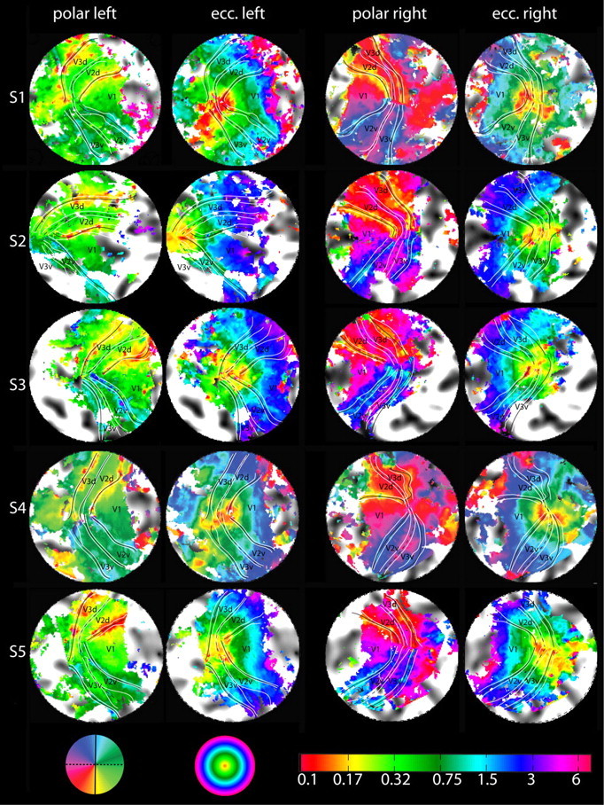
Retinotopic maps of all 10 hemispheres. The eccentricity maps are given on the left. Note the explicit eccentricity scale (bottom left) going down to 0.1° eccentricity. The polar angle maps are shown on the right. Vertical meridians are marked with continuous lines and horizontal meridians with dotted lines. The horizontal and vertical meridians and their confidence intervals (white) in this figure result from a bootstrapping analysis to estimate the spatial uncertainty of our measurement of visual area border. A high-resolution figure with and without these markings and one with manually identified borders are provided in the supplemental material, available at www.jneurosci.org.

Table 1.

Dimensions of the foveal confluence, showing the means and SDs across the hemispheres measured

	V2 width (mm)	V3 width (mm)	0.1° (mm2)
Mean	6.6	4.9	560
σ	±2.4	±1.9	±158

Consider first the vertical meridian representations forming the V1/V2 border and the approximately parallel anterior V3 border. These fiducial borders are coded as a yellow phase reversal in dorsal cortex and as a light blue phase reversal in ventral cortex, with a clear discontinuity where they meet the horizontal meridian (purple/red border) at the central foveal representation. In particular, the anterior border of ventral V3 can be identified by its representation of the upper vertical meridian (light blue). For dorsal V3, the representation of the anterior border can be identified by its representation of the lower vertical meridian (yellow). Note that the foveal ends of V3d and V3v form a continuous line with a clearly visible phase discontinuity from blue to yellow where they meet at the dorsal/ventral transition.

Figure 5 shows the results for each subject and hemisphere. Black lines indicate the area boundaries as estimated by a bootstrapping procedure; the 95% confidence intervals of these fits are marked by white lines. In most subjects, the area boundaries are reliable right into the foveal confluence with little or no overlap of the confidence intervals between adjacent areas. Except for S4 (right hemisphere V3d), each and every V3 quadrant border is clearly traceable even for eccentricities <0.5°. Thus, our high-resolution protocol was able to provide effective information about the layout of the cortical maps right into the foveolar representation.

To test if the stability of foveal boundary estimates was a result of peripheral data constraining the boundary fits, we removed phase information central to 0.5°. This exclusion resulted in the foveal boundary estimates becoming unreliable and in the confidence intervals increasing to larger than 20 mm (see supplemental materials, available at www.jneurosci.org). Hence, it is the phase information within the central 0.5° that provides the constraints responsible for keeping estimates of the areal boundaries from crossing or meeting in all hemispheres that we mapped (with only one exception).

Because of the intersubject variance in location, layout, and size of the early visual areas on cortex, the coverage of our high-resolution protocol was insufficient to resolve the outer border of V3 in some cases (especially in subjects with large brains). This typically impacted the ventral side of the maps as seen in subject S2 (Fig. 5), where the peripheral extent of V3v has been truncated slightly on the right but significantly on the left (hence missing much of V3v and part of V2v). Subjects S3 and S5 show a similar, albeit less pronounced, truncation. The representations of the horizontal and vertical meridians are the key features that inform the layout and borders of visual areas with the same color coding as in Figure 4. The top vertical meridians are color coded in light blue in both hemispheres in Figures 4, 5, and 8, although they are surrounded by blue in the left hemisphere and by dark green in the right hemisphere. Similarly, the lower vertical meridian representations are color coded in yellowish in Figures 4, 5, and 8 but are surrounded by red in the left hemisphere but by light green in the right hemisphere. These are the coding features that were used to guide the border assignations.

Close inspection of the polar map representations in Figure 5 reveals that in most of the hemispheres the foveal end of V3d and V3v form a continuous line with a clearly visible phase discontinuity where they meet. This phase discontinuity—signifying the switch from the upper to the lower visual field (i.e., from V3v to V3d)—is a prominent feature in almost all of our maps (see also the quantitative analysis in Fig. 6). Beyond the anterior border of V3 (dorsal and ventral), the data exhibit a further retinotopic coding with a return to horizontal phases (i.e., green phases for left hemispheres and purple phases for right hemispheres). Figure 6a provides an analysis of the phase discontinuity on the anterior border of V3 in the very center of the foveal representation—averaged across all subjects and hemispheres. It shows the estimated angular (red) and eccentricity (blue) location along the anterior V3 border, plotted against distance from the foveal center. The transition from upper vertical meridian representations (−90°) to lower vertical meridian representations (+90°) is within a few voxels (4 mm or ∼3 functional voxels). The eccentricity representation at these transitional voxels is <0.15°. This plot shows that the foveal part of V3 (dorsal and ventral) forms an elongated band of considerable length containing a fine eccentricity representation <1° of eccentricity.

Figure 6.

Quantitative analysis of isoeccentricity and isopolar lines. a, The vertical meridian representation that forms the anterior V3 border across all 10 measured hemispheres, as indicated by the red line in the pictogram on the left. The red curve shows the polar position estimate and the blue curve the eccentricity estimate, an ideal curve would be as step function switching from −90 to +90 in the center. The blue curve depicts eccentricity along the same line; here, the ideal curve would be V shaped. The data are averaged across subjects based on distance from the foveal center, with distance measured within the 3D surface reconstructions rather than in flattened patches. b, Polar position along isoeccentricity lines starting on the V1/V2 border, crossing V2 and V3, and ending at the anterior border of V3. Again, the position of the lines are depicted on the left. Ideally, the curves should be V shaped, too. Ventral curves should start at +90 and go down to 0, whereas dorsal curves should go from −90 to 0 and return to −90. Distance measurements are normalized to the mean length for this eccentricity. Filled circles represent data from the dorsal, squares from the ventral quarter field.

Figure 6b plots along the isoeccentricity lines, orthogonal to the meridian in 6a. Three eccentricities, 0.25, 0.5, and 1° ventral and dorsal are shown. The lines start at the V1/V2 border and stop at the anterior V3 border, demonstrating a polar phase profile that signifies V2 and V3. At both 0.25 and 0.5°, the combined bands of V2 and V3 span ∼12 mm, but at 1° eccentricity, they are considerably wider, spanning ∼20 mm. Thus, the plots in Figure 6 provide a quantitative analysis of the organization of the foveal confluence for V1–3.

The widths of the V2 and V3 bands were measured at their thinnest point in each hemisphere, where possible. An average width of 6.6 mm (σ = ±2.4 mm) was found for V2 and 4.9 mm (σ = ±1.9 mm) for V3. The surface area of the central-most region (eccentricities <0.1° comprising V1, V2, V3, and further anterior areas) was estimated to average 560 mm² (σ = ±158 mm²), also determined where possible.

Finally, using the Retinotopic Atlas Tools (Dougherty et al., 2003; Schira et al., 2007), a model of the representations of the visual field was fitted to those 6 of the 10 hemispheres with full coverage. This allowed estimation of a variety of numerical properties, in particular surface areas and magnification. We found that for foveal eccentricities <0.6°, both V2 (F = 138; p > 10⁻⁵) and V3 (F = 241; p > 10⁻⁵) had a significantly larger surface area than V1, as measured in the undistorted, folded 3D surface reconstruction rather than flatmap space. Conversely, for the parafoveal eccentricity range from 0.6 to 5°, the area for V1 was numerically larger than that for V2 and V3 (Fig. 7b), although this difference was not significant (F = 27; p = 0.065) in our data sample. This result is in line with previous work (Dougherty et al., 2003; Schira et al., 2007). Although V3 was slightly thinner than V2 in the foveal confluence, the estimated areas were similar for both (<0.6° only), suggesting that V3 is elongated relative to V2.

Figure 7.

Surface area analysis based on the six hemispheres with full coverage. a, Foveal magnification function; error bars depict the SE across measured hemispheres. For eccentricities of 1° and greater, V1 has a larger magnification than V2 or V3, but for 0.5° and below, both V2 and V3 are larger than V1. b, Surface areas in early visual areas for foveal representations (0–0.6°) and parafoveal representations (0.6–4.8°). For foveolar eccentricities V1 is significantly smaller than V2 and V3.

Discussion

High-resolution fMRI

Using high-resolution protocols for functional as well as anatomical data, we were able to achieve excellent data quality that overcame the partial voluming problem, a major confound in typical fMRI designs using resolutions of 3 × 3 × 3 mm³ or larger. Significant functional activity was restricted to cortical gray matter, whereas neighboring voxels sampling white matter contained little or no functional activity (Fig. 3a). A similar degree of functional isolation has been shown by previous studies (Logothetis and Pfeuffer, 2004; Ress et al., 2007) but not in an experiment designed explicitly to cover a significant volume of cortex and with the objective of investigating the functional organization of the cortical layout. For “everyday retinotopic mapping,” our experience shows that procedures consisting of two to four 5 min runs are sufficient. As a further conclusion from our study, we can also state that high-resolution fMRI is not only feasible but highly recommended for studies of functional organization using a standard 3T clinic/research scanner, a standard 8-channel head coil, and classic acquisition protocols.

Organization of the foveal confluence

Our data strongly support the conclusion that in the human cortex, areas V2 and V3 are separated and distinguishable from V1 and from each other, right up to the central representation of the visual field. They further suggest that, for both V2 and V3, the ventral and dorsal halves are connected to form a band through the very center of the foveal projection. These V2 and V3 bands surround the tip of V1, each being ∼6 mm wide (varying from 3 to 9 mm among subjects). Accordingly, a coarser resolution will not be able to resolve these structures. Finally, our data suggest that, beyond both the field sign reversals of the upper vertical meridian (anterior V3v border) and the lower vertical meridian (anterior V3d border) representations, the field sign of the polar angle map reverses again toward the horizontal meridian. Accordingly, in the human brain, our data indicate that V4 has no common border with V2, hence supporting the model proposed for the cortex of both marmoset and cebus monkeys (Piñon et al., 1998; Rosa and Tweedale, 2000, 2005). With respect to the V3 architecture, this organization is also in line with the model suggested by Hansen et al. (2007) in humans. This pattern was in agreement in both hemispheres of all subjects (except a single border in a single hemisphere, S4 RH; V3v). In this regard, it is important to note that no subjects were excluded from the analysis of Figures 5 and 6 because of inadequate data quality.

The cortical organization we observe is in disagreement with the maps usually reported for nonhuman primates—especially those for macaque monkey (Newsome et al., 1986; Maunsell and Van Essen, 1987; Gattass et al., 1988, 2005). However, close examination of those studies shows that the evidence on which these maps are based is far from conclusive, although they have become widely disseminated and are considered the dominant interpretation. As highlighted in the introduction there are, in fact, several studies suggesting a layout of the foveal confluence in other primate species very similar to our results (Piñon et al., 1998; Rosa et al., 2000; Rosa and Tweedale, 2000, 2005). This discrepancy among monkey studies could be a species difference, with a split organization of V3 in the macaque monkey but a continuous V3 organization for the cebus monkey and human. This would leave the organization in marmoset monkey under dispute, with some studies suggesting a split organization for V3 (Lyon and Kaas, 2001, 2002), whereas others imply a continuous V3 organization (Rosa and Tweedale, 2000, 2005).

Rather than treating this as an interspecies difference, one may group the studies based on the principle used to identify retinotopic areas. Studies relying on various histochemical staining patterns (Newsome et al., 1986; Maunsell and Van Essen, 1987; Gattass et al., 1988; Lyon and Kaas, 2002) suggest a split organization for V3, whereas those relying on field mapping (Piñon et al., 1998; Rosa et al., 2000; Rosa and Tweedale, 2000) suggest a continuous V3 organization consistent with the present study. Although Gattass et al. (1988) performed an extensive receptive field mapping in their study, they had to rely on “a myeloarchitectonic basis” for the organization of the foveal confluence. Myeloarchitecture is known to change within a visual area and in V3, in particular (Newsome et al., 1986), and hence may not provide the optimal criterion to address this question. Examination of the figures in Gattass et al. (1988) did not reveal a clear case for either organization, and careful reevaluation of the foveal organization in macaque, possibly using optical imaging techniques, may thus be required. This question is of great importance, since the interpretation of an organizational difference between human and cebus monkey on the one hand and macaque monkey on the other hand would have significant implications for our understanding of the phylogenesis of visual cortex in these species.

If we adhere to the principle that the same architecture should be expected to occur across primate species, characterization of the human visual system stands as an ideal approach to resolve this question, because the human visual cortex is vastly larger than that of any other primate. Accordingly, although V2 and V3 narrow to thin bands, they still yield structures with measurable widths of ∼6 mm. In comparison, less than a millimeter width has been suggested for marmoset monkey (Rosa and Tweedale, 2000). A second advantage of the human studies is the fact that human subjects can be easily instructed to perform accurate fixation over extended periods of time.

Proposed layout of the foveal confluence

Based on our data, together with other recent retinotopic mapping studies in human (Tyler et al., 2005; Larsson and Heeger, 2006; Hansen et al., 2007), we would like to propose the canonical model of the foveal confluence in human depicted in Figure 8. The main features are that V2 and V3 form continuous bands around the foveal singularity of V1 and that V3A and hV4 are both hemifield representation in the dorsal and ventral regions anterior to V3d and V3v, respectively. V3A seems to have a strong peripheral representation, whereas hV4 has a strong foveal representation adjacent to that of V3v.

The crossover of the magnification curves of V1 and V2/V3

Figure 7 shows that, <0.6° eccentricity, both V2 and V3 are larger than V1. Although surprising at first glance, this crossover is a necessary feature of the layout of the foveal confluence that we have identified. In Schira et al. (2007), we proposed a simple mathematical model of a retinocortical projection function that incorporated a constant ratio of the magnification of V1 and V2. This model would predict that the two halves of V2 continue to get narrower and narrower until they meet at a point singularity for the very central representation. Our present high-resolution results, however, reveal that V2 does not narrow down indefinitely but rather remains as a band of substantial width. In combination with the confluent eccentricity map, this layout must inevitably suggest a larger magnification for V2 (and V3) for regions foveal to some eccentricity, since V1 does indeed narrow down to a point.

hV4, V4d, and dorsal lateral occipital/lateral occipital 1

Although one might expect to find V4d and V4v anterior to the borders of V3d and V3v, respectively, Tootell and Hadjikhani (2001) reported that they could not identify the polar angle characteristics that they would expect from a V4d and questioned the existence of human V4d at the location suggested by nonhuman primate studies. In our data, however, the reversal of field map direction anterior of the representation of the lower vertical meridian is present in each and every case. The present study is far from being the first to report this feature (Tyler et al., 2005; Larsson and Heeger, 2006; Hansen et al., 2007). Tyler et al. (2005) interpreted this lateral occipital projection as an area containing an enlarged lower field representation and called it dorsal lateral occipital (DLO). Larsson and Heeger (2006) named this area lateral occipital 1 (LO1) and understand it as a part of a hemifield representation. Hansen et al. (2007) suggested that close to the foveal representation, this lower quarter field representation anterior to V3d corresponds to V4d, as described in nonhuman primates [challenging the interpretations by Tyler et al. (2005) and Larsson and Heeger (2006) but not their reported data]. Since some of the reported results may have been contaminated by partial voluming of the activation across sulci, we suggest that this area needs to be reexamined using high-resolution protocols. The present data cannot disambiguate this debate, since this area is often at the very edge of the coverage of the present high-resolution protocols and is rarely fully represented. We would nevertheless like to suggest that DLO/LO1/V4d extends alongside V3d right into the center of the foveal confluence.

Conclusion

Our high-resolution protocols and accurate fixation strategies allowed us to obtain clear retinotopic mapping data into the center of the foveal representations of retinotopic areas V1, V2, V3, and the adjacent cortical territory. Tracking the phase reversals corresponding to the horizontal and vertical meridian representations allowed us to establish that areas V2 and V3 in human cortex do not meet at a point but form continuous foveolar bands with a width of ∼6 mm in each case. For V3, in particular, this is a profoundly different view of its foveolar organization than the general consensus in various monkey species. We nevertheless suggest that this organization may not be incompatible with the sparse published data in those species and that the issue should be revisited with more definitive assessment techniques.

The fact that the V2 and V3 maps retain significant width in the foveolar region implies that they devote a larger area of cortex to the representation of the retina for eccentricities below ∼1° than does the V1 map. Interestingly, this approximately matches the extent of the foveal pit. This expansion of foveolar coverage in V2 and V3 opens up the possibility that there may be specialized processing for features and forms in the central fovea and suggests that detailed psychophysical measures of the foveolar magnification function may be used as a indicator of the operative processing level for particular visual tasks.

References

- Dougherty RF, Koch VM, Brewer AA, Fischer B, Modersitzki J, Wandell BA. Visual field representations and locations of visual areas V1/2/3 in human visual cortex. J Vis. 2003;3:586–598. doi: 10.1167/3.10.1. [DOI] [PubMed] [Google Scholar]
- Engel SA, Rumelhart DE, Wandell BA, Lee AT, Glover GH, Chichilnisky EJ, Shadlen MN. fMRI of human visual cortex. Nature. 1994;369:525. doi: 10.1038/369525a0. [DOI] [PubMed] [Google Scholar]
- Gattass R, Sousa AP, Gross CG. Visuotopic organization and extent of V3 and V4 of the macaque. J Neurosci. 1988;8:1831–1845. doi: 10.1523/JNEUROSCI.08-06-01831.1988. [DOI] [PMC free article] [PubMed] [Google Scholar]
- Gattass R, Nascimento-Silva S, Soares JG, Lima B, Jansen AK, Diogo AC, Farias MF, Botelho MM, Mariani OS, Azzi J, Fiorani M. Cortical visual areas in monkeys: location, topography, connections, columns, plasticity and cortical dynamics. Philos Trans R Soc Lond B Biol Sci. 2005;360:709–731. doi: 10.1098/rstb.2005.1629. [DOI] [PMC free article] [PubMed] [Google Scholar]
- Hansen KA, Kay KN, Gallant JL. Topographic organization in and near human visual area V4. J Neurosci. 2007;27:11896–11911. doi: 10.1523/JNEUROSCI.2991-07.2007. [DOI] [PMC free article] [PubMed] [Google Scholar]
- Larsson J, Heeger DJ. Two retinotopic visual areas in human lateral occipital cortex. J Neurosci. 2006;26:13128–13142. doi: 10.1523/JNEUROSCI.1657-06.2006. [DOI] [PMC free article] [PubMed] [Google Scholar]
- Logothetis NK, Pfeuffer J. On the nature of the BOLD fMRI contrast mechanism. Magn Reson Imaging. 2004;22:1517–1531. doi: 10.1016/j.mri.2004.10.018. [DOI] [PubMed] [Google Scholar]
- Lyon DC, Kaas JH. Connectional and architectonic evidence for dorsal and ventral V3, and dorsomedial area in marmoset monkeys. J Neurosci. 2001;21:249–261. doi: 10.1523/JNEUROSCI.21-01-00249.2001. [DOI] [PMC free article] [PubMed] [Google Scholar]
- Lyon DC, Kaas JH. Evidence for a modified V3 with dorsal and ventral halves in macaque monkeys. Neuron. 2002;33:453–461. doi: 10.1016/s0896-6273(02)00580-9. [DOI] [PubMed] [Google Scholar]
- Maunsell JH, Van Essen DC. Topographic organization of the middle temporal visual area in the macaque monkey: representational biases and the relationship to callosal connections and myeloarchitectonic boundaries. J Comp Neurol. 1987;266:535–555. doi: 10.1002/cne.902660407. [DOI] [PubMed] [Google Scholar]
- Newsome WT, Maunsell JH, Van Essen DC. Ventral posterior visual area of the macaque: visual topography and areal boundaries. J Comp Neurol. 1986;252:139–153. doi: 10.1002/cne.902520202. [DOI] [PubMed] [Google Scholar]
- Piñon MC, Gattass R, Sousa AP. Area V4 in Cebus monkey: extent and visuotopic organization. Cereb Cortex. 1998;8:685–701. doi: 10.1093/cercor/8.8.685. [DOI] [PubMed] [Google Scholar]
- Pruessmann KP, Weiger M, Scheidegger MB, Boesiger P. SENSE: sensitivity encoding for fast MRI. Magn Reson Med. 1999;42:952–962. [PubMed] [Google Scholar]
- Ress D, Glover GH, Liu J, Wandell B. Laminar profiles of functional activity in the human brain. Neuroimage. 2007;34:74–84. doi: 10.1016/j.neuroimage.2006.08.020. [DOI] [PubMed] [Google Scholar]
- Rosa MG, Tweedale R. Visual areas in lateral and ventral extrastriate cortices of the marmoset monkey. J Comp Neurol. 2000;422:621–651. doi: 10.1002/1096-9861(20000710)422:4<621::aid-cne10>3.0.co;2-e. [DOI] [PubMed] [Google Scholar]
- Rosa MG, Tweedale R. Brain maps, great and small: lessons from comparative studies of primate visual cortical organization. Philos Trans R Soc Lond B Biol Sci. 2005;360:665–691. doi: 10.1098/rstb.2005.1626. [DOI] [PMC free article] [PubMed] [Google Scholar]
- Rosa MG, Piñon MC, Gattass R, Sousa AP. “Third tier” ventral extrastriate cortex in the New World monkey, Cebus apella. Exp Brain Res. 2000;132:287–305. doi: 10.1007/s002210000344. [DOI] [PubMed] [Google Scholar]
- Schira MM, Wade AR, Tyler CW. Two-dimensional mapping of the central and parafoveal visual field to human visual cortex. J Neurophysiol. 2007;97:4284–4295. doi: 10.1152/jn.00972.2006. [DOI] [PubMed] [Google Scholar]
- Sereno MI, Dale AM, Reppas JB, Kwong KK, Belliveau JW, Brady TJ, Rosen BR, Tootell RB. Borders of multiple visual areas in humans revealed by functional magnetic resonance imaging. Science. 1995;268:889–893. doi: 10.1126/science.7754376. [DOI] [PubMed] [Google Scholar]
- Tootell RB, Hadjikhani N. Where is ‘dorsal V4’ in human visual cortex? Retinotopic, topographic and functional evidence. Cereb Cortex. 2001;11:298–311. doi: 10.1093/cercor/11.4.298. [DOI] [PubMed] [Google Scholar]
- Tyler CW, Likova LT, Chen CC, Kontsevich LL, Schira MM, Wade AR. Extended concepts of occipital retinotopy. Curr Med Imag Rev. 2005;1:319–329. [Google Scholar]
- Van Essen DC, Newsome WT, Maunsell JH, Bixby JL. The projections from striate cortex (V1) to areas V2 and V3 in the macaque monkey: asymmetries, areal boundaries, and patchy connections. J Comp Neurol. 1986;244:451–480. doi: 10.1002/cne.902440405. [DOI] [PubMed] [Google Scholar]
- Wandell BA, Dumoulin SO, Brewer AA. Visual field maps in human cortex. Neuron. 2007;56:366–383. doi: 10.1016/j.neuron.2007.10.012. [DOI] [PubMed] [Google Scholar]
- Zeki SM. Representation of central visual fields in prestriate cortex of monkey. Brain Res. 1969;14:271–291. doi: 10.1016/0006-8993(69)90110-3. [DOI] [PubMed] [Google Scholar]