How Connectivity, Background Activity, and Synaptic Properties Shape the Cross-Correlation between Spike Trains

Abstract

Functional interactions between neurons in vivo are often quantified by cross-correlation functions (CCFs) between their spike trains. It is therefore essential to understand quantitatively how CCFs are shaped by different factors, such as connectivity, synaptic parameters, and background activity. Here, we study the CCF between two neurons using analytical calculations and numerical simulations. We quantify the role of synaptic parameters, such as peak conductance, decay time, and reversal potential, and analyze how various patterns of connectivity influence CCF shapes. In particular, we find that the symmetry of the CCF distinguishes in general, but not always, the case of shared inputs between two neurons from the case in which they are directly synaptically connected. We systematically examine the influence of background synaptic inputs from the surrounding network that set the baseline firing statistics of the neurons and modulate their response properties. We find that variations in the background noise modify the amplitude of the cross-correlation function as strongly as variations of synaptic strength. In particular, we show that the postsynaptic neuron spiking regularity has a pronounced influence on CCF amplitude. This suggests an efficient and flexible mechanism for modulating functional interactions.

Introduction

Recordings of multineuron spike trains have revealed significant interdependencies between the firing of different neurons in a population (Zohary et al., 1994; Meister et al., 1995; Alonso et al., 1996; deCharms and Merzenich, 1996; Bair et al., 2001; Kohn and Smith, 2005). Although it is important to identify the role such functional interactions play in neural coding (Abbott and Dayan, 1999; Nirenberg et al., 2001; Nirenberg and Latham, 2003; Averbeck et al., 2006; Schneidman et al., 2006; Pillow et al., 2008), it is also important to understand how they depend on biophysical parameters and network activity (Poliakov et al., 1996, 1997; de la Rocha et al., 2007). For pairs of neurons, functional interactions are quantified by the cross-correlation function (CCF) between their spike trains, which measures how much the firing of one of the two neurons influences the firing of the other at different time lags. Statistically significant cross-correlations arise from the presence of a direct synaptic connection (Snider et al., 1998; Csicsvari et al., 1998; Barthó et al., 2004; Fujisawa et al., 2008) and/or from common or correlated inputs to the two neurons (Sears and Stagg, 1976; Binder and Powers, 2001; Constantinidis et al., 2001; Türker and Powers, 2001, 2002). The amplitude of the CCF therefore directly depends on the properties of the synapses mediating the interactions, but it is also modulated by the activity of the surrounding network (Aertsen et al., 1989; Poliakov et al., 1996; Constantinidis et al., 2001). The shape of the CCF also carries information on the underlying connectivity, yet inferring the circuitry from the CCF is a notoriously difficult problem (Melssen and Epping, 1987; Alonso and Martinez, 1998; Trong and Rieke, 2008). A detailed, quantitative understanding of the influences of synaptic parameters, network activity, and local circuitry on the CCF is therefore necessary for a correct interpretation of CCFs.

The basic influence of the underlying circuit on the shape of the CCF has long been considered at a qualitative level (Moore et al., 1970; Palm et al., 1988). More quantitative studies have been devoted to CCFs induced by a direct synaptic connection (Knox, 1974; Ashby and Zilm, 1982; Fetz and Gustafsson, 1983; Herrmann and Gerstner, 2002; Veredas et al., 2005). Early theoretical studies did not take into account the activity of the surrounding network, and it is only more recently that the effects of background inputs have been assessed using a phenomenological noise model (Herrmann and Gerstner, 2001). For the case of common inputs to the neurons, previous theoretical studies have concentrated on spike-count correlations (de la Rocha et al., 2007; Shea-Brown et al., 2008), and the results for the full CCF appear scarce (Kirkwood and Sears, 1978; Tchumatchenko et al., 2008).

In the present work, we systematically examine how the amplitude and time course of the CCF depend on the synaptic parameters, surrounding network activity, and local connectivity. To this end, we use pairs of integrate-and-fire neurons and represent the activity of the surrounding network by a compound, fluctuating background input that sets the baseline firing statistics of the neurons. We first show that the average firing response of a neuron to a given synaptic input strongly depends on the regularity of its firing. We next determine analytically the CCF in various simple microcircuits within a linear approximation. We first consider the two basic situations of a direct synaptic connection and common synaptic inputs to the two neurons. We then show how the results obtained for these two microcircuits can be used to study more complex ones, such as two mutually connected neurons and feedforward inhibition.

Materials and Methods

Integrate-and-fire models.

To study the influence of various biophysical parameters on the shape and amplitude of the cross-correlation function between the spike trains of two neurons, we used integrate-and-fire models in which action potentials are generated from the underlying dynamics of the membrane potential (Gerstner and Kistler, 2002). These dynamics are given by the following:

where the membrane potential V is determined with respect to the resting potential of the cell, c_m is the membrane capacitance of the neuron, g_m is the membrane conductance, g_mψ(V) is a spike-generating current, and I_syn is the total current elicited by synaptic inputs to the neuron. We used c_m = 250 pF and g_m = 25 nS. These parameters are taken from in vitro recordings from layer V neocortical pyramidal (Badel et al., 2008b), with g_m increased by a factor of 2–3 compared with in vitro values, to account for in vivo-type synaptic background inputs. We studied two different versions of the integrate-and-fire model.

In the leaky integrate-and-fire (LIF) model, ψ(V) = 0, there is no spike-generation current, and an action potential (AP) is emitted when the membrane potential crosses a fixed threshold value V_T. The membrane potential is subsequently reset to a value V_R. We did not introduce any refractory period after the emission of an AP. The values used for the threshold and reset were V_T = 20 mV and V_R = 10 mV.

In the exponential integrate-and-fire (EIF) model, the spike-generation current is exponential:

Once the membrane potential crosses the threshold V_T, it diverges to infinity in finite time. This divergence represents the firing of an action potential. After the divergence, the membrane potential is reset to a value V_R. The values used in this study were V_T = 10 mV and V_R = 3 mV. The parameter Δ_T quantifies the sharpness of the AP initiation. We took here Δ_T = 1 mV, a typical value for pyramidal cells (Badel et al., 2008b).

The LIF model (Lapicque, 1907) presents the advantage of being analytically tractable. However, the absence of spike-generating currents and the fixed threshold for spike emission may induce some differences with the behavior of conductance-based models. The EIF model, in contrast, reproduces in the simplest possible way the spike initiation in Hodgkin–Huxley type models (Fourcaud-Trocmé et al., 2003), the spike sharpness being described in the EIF model with a single parameter Δ_T. Moreover, it has been shown recently that the EIF model provides an excellent fit to in vitro dynamics of the membrane potential in cortical pyramidal neurons (Badel et al., 2008b), with a fitted value for the spike sharpness of Δ_T = ∼1 mV.

If the neuron receives a constant input current I_syn(t) = −I₀, we find it useful to define the effective rest potential μ = I₀/g_m as the value the membrane potential of the neuron would reach in the absence of threshold and spike-generating mechanisms.

Spike-train statistics and the cross-correlation function.

A spike train is represented as the following time series:

where t_j for j = 1,…, p is the series of spike times ordered in time on the interval [0,T]. It is often useful to work with Fourier transforms ñ(ω) = [n] of spike trains, the Fourier transform of a function f being defined as follows:

so that

The instantaneous firing rate ν(t) is defined as follows:

where the brackets denote averaging over trials. If the firing is stationary, ν(t) = ν₀ for all t.

For stationary firing, the regularity of the spike train is quantified using the coefficient of variation (CV), defined as follows:

where Δt_j = t_j−t_{j −1} is the jth interspike interval, and the bar denotes averaging over all interspike intervals in the spike train.

The autocorrelation function of a spike train is defined as follows:

The Fourier transform of A(t), Ã(ω), is equal to the power spectrum of the spike train. It is given by the following:

The cross-correlation function between the spike trains n⁽¹⁾(t) and n⁽²⁾(t) of two neurons is as follows:

The value of C(t) represents the variation of the firing rate of the neuron 2, conditioned on the fact that neuron 1 fires t milliseconds earlier. With the normalization adopted here, this variation is expressed as the fraction of the baseline firing rate of neuron 2. Note that the normalization used here is different from the normalization by the geometric mean $\sqrt{{\nu }_0^{(1)}{\nu }_0^{(2)}}$ of the firing rates, commonly used for spike-count correlations (Bair, 2001; Kohn and Smith, 2005; de la Rocha et al., 2007).

The Fourier transform C̃(ω) of C(t), also called the cross-spectrum between neurons 1 and 2 is given by the following:

In this study, we determine C̃(ω) analytically and then recover C(t) using the inverse Fourier transform.

Synaptic inputs.

Synaptic inputs are modeled as transient conductance increases that cause a voltage-dependent inward or outward current flow in the postsynaptic neuron. More precisely, the postsynaptic current (PSC) elicited by a single presynaptic AP at time t₀ is given by the following:

where E_syn is the synaptic reversal potential, and g_syn is the conductance of a synapse. The time evolution of g_syn after a presynaptic spike is given by a delayed exponential:

Here g₀ is the peak conductance, and δ_s and τ_s are the latency and decay time. Unless otherwise indicated, the values of the synaptic times are δ_s = 1.5 ms (Markram et al., 1997) and τ_s = 3 ms (Hestrin, 1993).

The maximum amplitude of the postsynaptic current fluctuates from presynaptic spike to presynaptic spike because of the voltage dependence in Equation 12. Its mean is given by (μ − E_syn)g₀, where μ is the effective rest potential of the neuron. E_syn − μ represents the effective driving force of a synapse with reversal potential E_syn in the presence of fluctuating inputs.

Background synaptic activity.

Each cortical neuron receives a large number of synapses from other neurons, the typical estimate of this number being of the order of tens of thousands (Braitenberg and Schüz, 1991). In vivo, neurons are spontaneously active so that any neuron receives persistent background inputs as a result of the firing of its afferents. To study the effect of this background activity on cross-correlation functions, we represent it as a compound background input to the neurons, as precisely described below.

If the amplitude of each postsynaptic current is small with respect to the threshold for spike generation, a large number of synaptic events is needed to cause the firing of an action potential. In such a situation, the cumulative conductance of many co-occurring synaptic inputs generated from random background activity can be described as a Gaussian random process, the so-called diffusion approximation (Tuckwell, 1988).

More precisely, in the case in which the neuron receives two types of synaptic inputs, excitatory and inhibitory ones, for each type of input, the total conductance attributable to background synaptic activity can be expressed as a sum of a tonic and a fluctuating part as follows:

where g₀^E and g₀^I are the mean background synaptic conductances, respectively, for the excitatory (E) and the inhibitory (I) synapses, σ_g^E and σ_g^I are the SDs of the background synaptic conductances, and η^E(t) and η^I(t) are Gaussian stochastic processes of zero mean and unit SD. For the sake of analytical understanding, we assume that η^E and η^I are uncorrelated in time, i.e., η^E and η^I are white-noise processes, although this is generally not the case because of the presence of the nonvanishing synaptic decay times τ_s. Including a finite correlation time in the background inputs modifies qualitatively the behavior of the LIF model (Brunel et al., 2001) but not the behavior of the EIF model (Fourcaud-Trocmé et al., 2003) or of cortical neurons in vitro (Köndgen et al., 2008).

The total postsynaptic current attributable to the background synaptic inputs is given by the following:

where E_E and E_I are the reversal potentials of excitatory and inhibitory synapses. This current can be decomposed in a sum of a voltage-independent term and a voltage-dependent term. Within the diffusion approximation, the voltage-independent term is described by a tonic and a fluctuating part as follows:

where the mean I₀ and the SD σ can be expressed in terms of g₀^E, g₀^I, σ_g^E, and σ_g^I and the synaptic reversal potentials E_E and E_I (Richardson, 2004). This is the background synaptic current term in Equation 1. Throughout this study, we examine only the stationary situation in which I₀ and σ are constant. Note that σ is expressed in millivolt units. In the absence of firing threshold, the SD of the membrane potential is equal to σ/$\sqrt{2}$.

The voltage dependent part is simply given by (g₀^E + g₀^I)V, i.e., it has no fluctuating part within the diffusion approximation (Richardson, 2004; Richardson and Gerstner, 2005). The only effect of the voltage-dependent part is thus to modify tonically the membrane conductance of the neuron, in a time-independent manner. We therefore incorporate this effect in the model by setting g_m to a value larger than typically measured in vitro in the absence of background inputs.

Linear response to synaptic inputs.

To evaluate the cross-correlation function between the spike trains of two neurons, we need to quantify how much a conductance change attributable to a single synapse modifies the instantaneous firing rate of a postsynaptic neuron that is in a stationary state. The current elicited by a synaptic conductance change g(t) is as follows:

where E_syn is the synaptic reversal potential.

We assume that the amplitude of this postsynaptic current is small so that the resulting variation of the firing rate is small, too, and can be described as a linear variation around the stationary firing rate:

Here we have averaged over trials, the conductance variation being identical in all trials; ν₀ is the baseline firing rate attributable to tonic background inputs, and R_n is the linear response kernel to a synaptic conductance variation. A similar technique was used previously (Lindner et al., 2005). The linear response approximation can be written in frequency as follows:

where R̃_n = [R_n] is the linear response in frequency, and g̃ = [g].

The postsynaptic current in Equation 18 can be decomposed in a sum of two components, a component −g(t)E_syn independent of the membrane potential of the postsynaptic cell, and a component g(t)V proportional to the membrane potential and equivalent to a variation of the membrane conductance. Correspondingly, the linear response to a synaptic input can therefore be expressed as follows:

where R_E is the linear response kernel to a variation of the input current to the postsynaptic cell, μ is the effective rest potential of the neuron, and R_shunt is the linear response kernel to a variation of its membrane conductance. Equivalently, for the response in frequency, we write R̃_n = R̃_E(E_syn − μ) + R̃_shunt.

If E_syn is significantly different from μ, the total linear response is dominated by R_E:

The linear response function R_E is closely related to the Wiener kernel of the neuron (Poliakov et al., 1997) and the spike-triggered average (STA) input current (Paninski, 2006) as described in Appendix B. The full linear response kernel R_n is calculated in Appendix A.

Dominant timescale approximation for R_n.

The linear kernel R_n can be written as follows:

where {a_j} and {z_j} are complex numbers, with 0 > Re(z₁) > Re(z₂)… (for more details, see Appendix C).

The dominant timescale approximation consists in keeping only the long time asymptotic behavior for R_n(t), i.e., the exponential of the pole z₁ with the least negative real part. If the SD σ of the background noise term is small, the dominant pole has a nonzero imaginary part, and we write it as z₁ = −1/τ₁ + iω₀. In the dominant pole approximation, R_n becomes as follows:

If σ is larger than a critical value, z₁ becomes real, and we write it as z₁ = −1/τ₁, so that in the dominant pole approximation, the following holds true:

Results

Firing-rate responses to current and conductance variations

The cross-correlation function between the spike trains of two neurons quantifies the average temporal variation of the firing rate of one neuron relatively to the firing time of the other neuron (Perkel et al., 1967). This variation of the firing rate around its baseline value is ultimately attributable to synaptic inputs, arising for example from a direct synapse between the two neurons or from common or correlated inputs to the two neurons. To describe the cross-correlation function in any circuit, one thus first needs to quantify the effect of a change of its input synaptic conductance on the firing rate of a neuron. It is important to note that the average response to a given synaptic input depends on the baseline state of the neuron, i.e., its baseline firing rate ν₀ but also the regularity of this firing as quantified by its CV. These properties of the baseline state are set by the background synaptic inputs to the neuron. We therefore systematically examine the influence of stationary background inputs (see Materials and Methods) on the response properties of the neuron.

If the amplitude of the input conductance variation is small compared with the firing threshold of the neuron—as is often the case when only a subset of presynaptic neurons fires—the corresponding variation of the firing rate is proportional to amplitude of the conductance variation and can be described by the linear response of the firing rate of the neuron to synaptic inputs (see Materials and Methods), i.e., the temporal filter mapping the synaptic conductance variation to a variation of the firing rate. This linear filter can be specified either in time by the firing-rate response function R_n or in frequency by the Fourier transform of R_n denoted R̃_n. Before studying cross-correlation functions, we describe here the properties of R_n and R̃_n for two models of neurons, leaky integrate-and-fire and exponential integrate-and-fire, in the presence of background synaptic noise that induces a baseline firing specified by its frequency ν₀ and CV. To disentangle the influence on the response of the baseline firing rate ν₀ and baseline firing regularity, while varying the SD σ of background noise, we systematically adjust the mean input to keep ν₀ constant. Increasing σ then results in increasing the CV at fixed firing rate (Fig. 1D).

Figure 1.

Neuronal firing rate response to varying input current, for the leaky integrate-and-fire model (left column) and the exponential integrate-and-fire model (right column). A, Modulus of the response R_E as function of input frequency for two values of background noise corresponding to regular firing (CV = 0.2; LIF, σ = 0.5 mV; EIF, σ = 1 mV) and irregular firing (CV = 0.8; LIF, σ = 6 mV; EIF, σ = 8 mV). The dashed line represents the asymptotic decay at large frequencies. B, Phase of R̃_E. C, Response in time R_E(t), for the two values of background noise. The dashed line represents the dominant time approximation 2a₁ exp(−t/τ₁) in the case of large noise. D, CV of the interspike intervals as function of the SD σ of background synaptic noise. E, Gain as function of σ. The gain is defined as a the value of R̃_E at zero frequency. It corresponds to the slope of the f–I curve of the neuron at firing rate ν₀ and given level of background noise σ. F, Dominant decay time τ₁ as function of σ. In A–C, the firing rate is 30 Hz. In D–F, the baseline firing rate is maintained constant by adjusting the mean input current as σ is varied.

The response function R_n can be written as follows:

where μ is the effective rest potential, R_E is the firing-rate response to a varying input current, and R_shunt is the response to a variation of the membrane conductance (for additional details, see Materials and Methods). If the synaptic reversal potential E_syn is sufficiently different from the effective rest potential μ, i.e., if E_syn − μ is large, the response function R_n to a synaptic input is essentially equivalent to the response to a varying input current R_E. Conversely, if E_syn is close to μ, then R_n depends strongly on the response R_shunt to a variation of the membrane conductance. We therefore describe R_E and R_shunt separately in the following.

Response to current modulations

The linear response function R̃_E to input current modulations of different frequencies has been studied theoretically (Brunel et al., 2001; Fourcaud-Trocmé et al., 2003; Richardson, 2007) and experimentally (Köndgen et al., 2008; Boucsein et al., 2009), whereas its equivalent in time R_E is closely related to the Wiener kernel (Poliakov et al., 1997) and the STA current of the neuron (Paninski, 2006; Badel et al., 2008a) (see Appendix).

For both LIF and EIF models, the response R̃_E to modulated current is essentially a low-pass filter, the cutoff frequency of which decreases with increasing background synaptic noise. For low background synaptic noise (CV ≲ 0.5), R̃_E(ω) displays resonances at frequencies multiple of the underlying baseline firing frequency ν₀ (Fig. 1A), and the response in time R_E(t) displays oscillations at a frequency equal to the baseline firing frequency ν₀ (Fig. 1C). Qualitatively, in this regime in which the neuron spikes regularly with a period T, the effect of a given input at time t₀ is to shift the times of the following spike emissions. Specifically, for the LIF and EIF neurons, an excitatory input advances the next spike, especially when this spike follows closely the input arrival. The effect is to increase the probability of spike emission at the input time t₀ and, because spikes are emitted regularly, also at times that follow it by an integer number of periods (t₀ + T, t₀ + 2T,…). Correlatively, between these regularly spaced times when probability of spike emission is increased, the differential shift of spike time by the input decreases the probability of spike emission. For high background noise (CV ≳ 0.5), R̃_E(ω) is instead a pure low-pass filter with a cutoff frequency of the order of ν₀, and R_E(t) decays monotonically (Fig. 1C). Qualitatively, for high background noise, an excitatory input at time t₀ simply increases the probability of spike emission in a time range after t₀.

The time course of R_E at short times is determined by the asymptotic behavior of R̃_E at high frequencies. For the leaky integrate-and-fire model, the amplitude of R̃_E decays asymptotically as 1/$\sqrt{\omega }$ (Brunel and Hakim, 1999), so that R_E diverges as 1/$\sqrt{t}$ in the limit t → 0 (Paninski, 2006). This divergence implies that the LIF model is capable of responding fast to current variations. In contrast, for the exponential integrate-and-fire model, the amplitude of R̃_E decays asymptotically as 1/w (Fourcaud-Trocmé et al., 2003), so that R_E reaches a finite limit at zero times (Fig. 1C). The response of the EIF model is therefore slower at short times than the response of the LIF model.

The asymptotic behavior of R_E(t) at long times can be described using the dominant mode approximation (see Materials and Methods and Appendix C). For high background noise, this approximation predicts that R_E(t) decays exponentially with a time constant τ₁ that can be calculated from Equation 49 (Appendix B). This time constant determines the longest timescale in the dynamics of the firing rate and sets a limit on the rate of variation of the firing frequency in response to a varying input current. Interestingly, the value of τ₁ depends on the input statistics, i.e., on the SD of the background noise σ and the baseline firing frequency ν₀ of the neuron. In Figure 1F, the time constant τ₁ is displayed as a function of the SD of background noise σ, the firing rate ν₀ being held constant by adjusting the mean background input while σ is varied. For the LIF model, τ₁ increases with σ, whereas for the EIF model, it reaches a maximum at intermediate values of σ and decreases for larger values of σ. In both models, τ₁ decreases with increasing ν₀. In particular, it appears to be always smaller than the membrane time constant τ_m.

The amplitude σ of the background noise strongly modulates the amplitude of the response and affects differently the response at low and high frequencies. The response R̃_E at low frequencies is given by the gain of the neuron, i.e., the variation of its background firing rate when its mean input current is changed. The gain of a neuron is known to depend on the amplitude of background noise (Chance et al., 2002). Figure 1E shows that, for both models studied, the gain decreases with increasing σ, the magnitude of this variation being dependent on the baseline firing rate ν₀. The effect of noise on the amplitude of the response at high frequencies is different from its effect on the gain but depends on the model: for the LIF model, R̃_E (ω) scales as 1/σ for large ω, whereas for the EIF model, it is independent of σ (Fourcaud-Trocmé et al., 2003).

Response to membrane conductance modulations

If the synaptic reversal potential E_syn is close to the effective rest potential μ of the neuron, the membrane conductance variation after a synaptic input plays an important role in the firing rate response. In particular, if E_syn is exactly equal to the effective rest potential μ, then the firing rate response is entirely attributable to shunting, i.e., R̃_n = R̃_shunt. The influence of the variation of membrane conductance on the firing response can be understood in the LIF model as a superposition of two effects, a variation of the membrane timescale of the neuron, and a variation of the amplitude of the fluctuating input (for details, see Appendix A). These two effects compete against each other: increasing the conductance decreases the effective time constant, leading to an instantaneous increase of the firing rate, but it also decreases the effective level of noise, the effect of which depends on whether the mean input is subthreshold (μ below the threshold V_T) or suprathreshold (μ > V_T). In the case of subthreshold input, the shunting part R_shunt of the linear response in time R_n is biphasic, with a fast negative part and a slower positive part. In contrast, for suprathreshold inputs, R_n is positive at all times. These two cases are illustrated in Figure 2, where ν₀ = 30 Hz corresponds to a subthreshold input and ν₀ = 65 Hz corresponds to a suprathreshold input.

Figure 2.

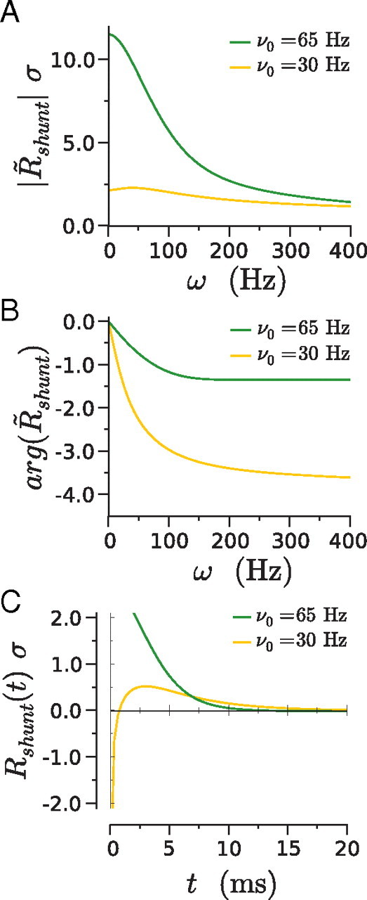
Linear response of the instantaneous firing rate of an LIF neuron to a membrane conductance variation, in the case of subthreshold inputs (ν₀ = 30 Hz) and suprathreshold inputs (ν₀ = 65 Hz). A, Modulus of the response R̃_shunt to different input frequencies. B, Phase of R̃_shunt. C, Linear response in time, R_shunt(t). The SD of background noise is σ = 6 mV.

In summary, in this section, we have examined the firing-rate response of a neuron to a time-varying conductance input. We have shown that both the amplitude and the timescales of this response strongly depend on the baseline firing statistics of the neuron, set by the background synaptic input.

Correlations arising from a direct synaptic connection

Having characterized the response of a neuron to synaptic inputs, we now turn to the cross-correlation function between spike trains of two neurons arranged in different circuits. We first examine the cross-correlations attributable to a direct synaptic connection between two neurons (Fig. 3). Assuming that both the presynaptic and the postsynaptic neuron receive background synaptic inputs uncorrelated from each other, the cross-spectrum can be expressed as follows:

where R̃_n is the linear response function of the postsynaptic neuron (see previous section) (Figs. 1, 2), g̃_syn is the Fourier transform of the synaptic conductance time course after a single presynaptic spike (see Materials and Methods), Ã_pre(ω) is the power spectrum of the spike train of the presynaptic neuron, and ν₀^(pre) (resp. ν₀^(post)) is the stationary firing rate of the presynaptic (resp. postsynaptic) neuron. Details of the derivation are provided in Appendix D.

Figure 3.

Cross-correlation function C(t) arising from a direct synaptic connection between the two neurons, in the case of current-dominated inputs ( E_syn − μ ≫ 1). The presynaptic neuron is a Poisson process and the postsynaptic neuron an LIF (left column) or an EIF (right column). A, Time course of the cross-correlation function C(t) for low background synaptic noise, corresponding to a CV of 0.2 (LIF, σ = 0.5 mV, PSC amplitude of 15 pA; EIF, σ = 1 mV, PSC amplitude of 25 pA). For comparison, the time course of the postsynaptic current is shown in orange (rescaled in arbitrary units). The histogram displays results of direct numerical simulations. B, Same as in A, in the case of high background synaptic noise, corresponding to a CV of 0.8 (LIF, σ = 6 mV, PSC amplitude of 100 pA; EIF, σ = 8 mV, PSC amplitude of 125 pA). The dashed trace shows the dominant timescale approximation for C(t). In A and B, the baseline firing rate of the postsynaptic neuron is 30 Hz. C, D, Peak value and peak time of C(t), as function of the synaptic decay time τ_s, for CV = 0.8. E, F, Peak value (log scale) and peak time of C(t), as function of the SD σ of background synaptic noise. While varying σ, the firing rate ν₀ was kept constant by adjusting the mean input current. Results in C–F are shown for three different values of the firing rate ν₀ (10, 30, and 50 Hz as described by the legend in E). The synaptic decay time was τ_s = 3 ms, except in C and D. The amplitude of the postsynaptic current was 60 pA (corresponding to a peak postsynaptic potential of 0.5 mV), except in A and B.

Because R̃_n = R̃_E(E_syn − μ) + R̃_shunt, the cross-correlation function can be written as C(t) = C_E(t) + C_shunt(t), with C_E(t) purely induced by current variations and proportional to the amplitude g₀(E_syn − μ) of the postsynaptic current and C_shunt(t) purely induced by membrane conductance variations and proportional to the peak synaptic conductance g₀. If E_syn − μ is large enough, C_shunt(t) is negligible with respect to C_E(t). We therefore first examine current-induced cross-correlations and later examine the influence of conductance variations for E_syn close to μ. Note that C_E(t) is proportional to (E_syn − μ), the sign of which determines whether the synapse is excitatory or inhibitory.

Poisson presynaptic firing

It is instructive to consider first the situation in which the firing of the presynaptic neuron is a Poisson process, in which case the power spectrum Ã_pre(ω) is a constant. The cross-correlation function C_E(t) is then simply given by the synaptic conductance time course filtered through the linear response function R_n. In particular, C_E(t) at negative times is necessarily zero, and a nonzero synaptic delay δ_s simply shifts C_E(t) by δ_s to positive times.

Because R_E filters out high frequencies (Fig. 1A,B), the time course of current-induced cross-correlations is always slower than the time course of the postsynaptic current (Fig. 3A,B). For low background noise (Fig. 3A), the resonances in R̃_E (Fig. 1A) lead to secondary peaks at positive times in the cross-correlation function C_E(t), located at multiples of the baseline firing frequency ν₀. For high background noise, C_E(t) displays a single peak as shown in Figure 3B. In that case, within the dominant timescale approximation, the cross-correlation function can be expressed as a difference of two exponentials:

where δ_s and τ_s are the latency and the decay time of the synaptic conductance, τ₁ is the dominant timescale in R_n(t) (Fig. 1C), and C₀ is a constant given in Appendix C. Figure 3B shows that the dominant mode approximation describes well the asymptotic decay of C_E(t) at large times, the timescale of that decay being given by the maximum between the neuronal timescale τ₁ and the synaptic timescale τ_s as seen from Equation 28. The dominant approximation, however, fails to describe the small time behavior of C_E(t), which is determined by the fast components of R_E(t) at small t. The main difference between the LIF and the EIF model is that, for the LIF model, R_E diverges at small t, which leads to a fast rise of C_E(t) at small t, whereas in the EIF model, R_E remains finite and correspondingly the rise C_E(t) at small t is slower. Despite this qualitative difference at short times, the CCFs for the two models end up looking very similar (Fig. 3, compare both B panels). This is in part attributable to the fact that, for the values of the noise used in Figure 3B, the dominant timescale τ₁ is very similar in both models.

The peak time and amplitude of the cross-correlation function C_E(t) naturally depend on the biophysical parameters of the synaptic connection, its peak conductance g₀, and decay timescale τ_s. Because we are using a linear approximation, the amplitude of C_E(t) is proportional to g₀. In Figure 4, we examine the accuracy of the linear approximation by comparing our theoretical predictions with numerical simulations for different values of the PSC amplitude g₀(μ − E_syn). The level of accuracy of the linear approximation depends on the ratio between the PSC amplitude and the noise amplitude: for high noise, the approximation is excellent over a wide range of physiological PSC amplitudes; in contrast, for low noise, deviations are seen for large PSCs. Note that the linear approximation does not capture the asymmetry between inhibitory and excitatory CCFs, as pointed out previously (Herrmann and Gerstner, 2001).

Figure 4.

Testing the validity of the linear approximation in the case of a direct synaptic connection between two LIF neurons: the theoretical predictions based on the linear approximation (black traces) are compared with numerically estimated cross-correlation functions, obtained by varying the amplitude g₀(E_syn − μ) of the PSC (color scale). On the vertical axis, the CCF amplitude is rescaled by the PSC amplitude g₀(E_syn − μ). Left, Low noise, CV = 0.2, σ = 0.5 mV; right, high noise, CV = 0.8, σ = 6 mV. The color scale is the same in both panels, and the firing rate is 30 Hz. The insets display the amplitude of the CCF as function of the PSC amplitude compared with the linear prediction (black line).

Because the cross-correlation function is a filtered version of the synaptic conductance time course, its peak time and amplitude increase with τ_s as seen in Figure 3, C and D. For fixed g₀, longer-lasting postsynaptic currents thus have a stronger effect on the firing of the postsynaptic neuron. Such a dependence is qualitatively described by the dominant timescale approximation (see Appendix D), although this approximation is not very accurate quantitatively.

The peak time and amplitude of the cross-correlation function are not set by the synaptic properties alone but depend strongly on the statistics of baseline firing of the postsynaptic neuron. The effect of the background synaptic noise amplitude is shown in Figure 3E. The neuron firing rate is kept fixed by adjusting the mean input so that only its CV varies with the noise amplitude. Remarkably, one sees that, for the LIF model, the cross-correlation amplitude decreases inversely proportionally to the SD σ of the background noise. In other words, the regularity of the baseline firing of the postsynaptic neuron has a strong influence on the amplitude of the cross-correlations: for a given synaptic peak conductance and decay time, the more regularly the postsynaptic neuron fires, the larger the cross-correlation amplitude. This is also true for the EIF model, although in that model the modulation of the cross-correlation amplitude with noise strength is somewhat weaker, as shown in Figure 3E. For both models, the cross-correlation amplitude decreases with increasing baseline firing rate ν₀, but varying ν₀ modulates the cross-correlation amplitude in a weaker manner than varying σ. Conversely, the peak time of C(t) is relatively insensitive to σ, for both LIF and EIF models. The peak time decreases with increasing firing rate, in agreement with the predictions of the dominant timescale approximation.

For the sake of comparison with experimental studies, in Figure 3, C and E, the peak value of the cross-correlation function is given for a synaptic conductance corresponding to a postsynaptic current amplitude of 60 pA and a synaptic decay time τ_s = 3 ms, yielding a postsynaptic potential (PSP) peak of 0.5 mV, a typical order of magnitude for AMPA-dependent EPSPs in the cortex (Markram et al., 1997; Sjöström et al., 2001; Holmgren et al., 2003; Barbour et al., 2007). For background synaptic inputs corresponding to a firing rate ν₀ = 30 Hz and CV = 0.9 (σ = 8 mV in the LIF model), our analysis predicts a corresponding peak cross-correlation of 0.15, meaning that the synaptic inputs from the presynaptic neuron increase the firing rate of the postsynaptic neuron by 15% with respect to the baseline firing rate. If the background noise amplitude is reduced by half to σ = 4 mV, the CV becomes 0.7, but the amplitude of the cross-correlations increases to 0.3.

Influence of the firing statistics of the presynaptic neuron

If the firing of the presynaptic neuron is not poissonian, the autocorrelation of the presynaptic firing also plays a role in the cross-correlation function (see Eq. 27). We examined the effect of the presynaptic autocorrelation for the LIF models, for which the power spectrum Ã_pre(ω) can be analytically calculated (see Appendix E). Depending on the level of background synaptic noise, the LIF neuron can be found in one of the three following regimes, illustrated in Figure 5A: (1) for weak background noise (CV < 0.5), the neuron fires rhythmically, and its autocorrelation function exhibits peaks at multiples of the mean interspike interval; (2) for intermediate background noise (0.5 < CV < 1), the presynaptic neuron fires irregularly but exhibits a noise-dependent refractory period around zero in the autocorrelation function; (3) for strong background noise (CV > 1), the neuron tends to fire in bursts, which results in positive autocorrelation at short time lags. The effect of the presynaptic autocorrelation on the cross-correlation function is most prominent at negative times (corresponding to the postsynaptic neuron firing before the presynaptic one), in which C(t) is essentially given by the autocorrelation function of the presynaptic neuron. This is illustrated in Figure 5B in the three firing regimes of the presynaptic neuron. For weak noise in the presynaptic neuron, C(t) displays periodic secondary peaks at both positive and negative times, corresponding to the period T in the firing of the presynaptic neuron. The peaks correspond to increased postsynaptic spiking arising from the spikes at (…, −2T, −T, 0, T, 2T, …) in the presynaptic neuron. For intermediate noise in the presynaptic neuron, regular spiking disappears and C(t) simply displays a dip close to zero attributable to the refractory period of the presynaptic neuron. For strong noise in the presynaptic neuron, C(t) displays positive values close to zero as a result of the bursts in the presynaptic neuron. It is important to note that the firing statistics of the presynaptic neuron affect only marginally the amplitude of the cross-correlation function, in contrast to the firing statistics of the postsynaptic neuron. Interestingly, the amplitude of the CCFs increase when presynaptic CV increases, whereas it decreases when postsynaptic CV increases. Figure 5C displays the effect of the presynaptic firing rate on C(t) at intermediate presynaptic noise: the effect of the presynaptic refractory period increases with increasing presynaptic firing rate.

Figure 5.

Effect of the autocorrelation of presynaptic firing on the cross-correlation function C(t) in the case of a direct synaptic connection between the neurons. Both neurons are LIF neurons, receiving independent background inputs with different statistics. A, Autocorrelation function of the presynaptic spike train for low, intermediate, and high background noise. B, Corresponding cross-correlation function C(t) compared with C(t) obtained for a poissonian presynaptic spike train. The postsynaptic neuron receives an intermediate level (CV = 0.8, σ = 6 mV) of synaptic noise, and both neurons are firing at a stationary rate of 30 Hz. C, C(t) for three different values of the presynaptic firing rate ν_pre, for moderate background noise in both neurons (σ = 6 mV). The anti-correlations at negative times increase with ν_pre. In B and C, the PSC amplitude is 30 pA.

Shunting effects

If the synaptic reversal potential E_syn is close to the effective resting potential μ of the postsynaptic neuron, the membrane conductance variations have an important influence on the cross-correlation function. Figure 6 displays the total cross-correlation function C(t) = C_E(t) + C_shunt(t) for E_syn close to the effective rest potential μ. For E_syn = μ, at the point of crossing between inhibition and excitation, the full cross-correlation is given by C_shunt. If the input is subthreshold (μ < V_T), R_shunt is biphasic, so that C(t) is biphasic with a fast inhibitory phase at small times and a slower excitatory phase at long times (Fig. 6A). For E_syn close to μ, depending on the sign of E_syn − μ, the excitatory or inhibitory phase of C_shunt(t) is amplified by the cross-correlation C_E(t) arising from current variations. For E_syn − μ, negative but small C_E(t) approximately cancels the slow excitatory phase of C_shunt, and only the fast inhibitory part of C_shunt remains in C(t). Note that this inhibitory part is as fast as the postsynaptic current and thus significantly faster than cross-correlations arising from current variations alone.

Figure 6.

Effects of shunting on the cross-correlation function for an LIF model. A, Cross-correlation function C(t) arising from a direct synaptic connection, in the case when the synaptic reversal potential is close to the effective rest potential μ of the postsynaptic cell. For E_syn = μ, the cross-correlation function is a result of shunting alone. B, Comparison between the full cross-correlation function C(t) (solid lines) and the cross-correlations C_E resulting from current inputs (dashed line). Shunting accelerates the cross-correlation function in the case of inhibition and delays it in the case of excitation. In A and B, the mean input is subthreshold, with ν₀ = 30 Hz and σ = 6 mV. C, D, Same as in A and B, but for a suprathreshold input (ν₀ = 65 Hz and σ = 6 mV). In all panels, g₀ = 8 nS.

If the input is suprathreshold, R_shunt is monophasic, and C_shunt(t) is purely excitatory for E_syn = μ. C(t) becomes biphasic when the effective resting potential μ is slightly below the synaptic reversal potential (Fig. 5C) arising from a competition between an excitatory shunting effect and an inhibitory effect arising from the negative effective driving force. The average background level at which the transition between an excitatory and an inhibitory CCF occurs thus depends on the baseline firing rate.

If the effective driving force E_syn − μ is of the order of tens of millivolts, current variations dominate, and shunting hardly affects the amplitude of C(t). However, it modifies the time course of C(t) with respect to the CCF C_E(t) purely induced by current variations: the time course of C(t) is faster than that of C_E(t) in the case of inhibition and slower in the case of excitation. This is illustrated in Figure 6B for subthreshold inputs and E_syn − μ = 10 mV and in Figure 6D for suprathreshold input and E_syn − μ = 30 mV.

To summarize, we have shown that the primary peak in the cross-correlation function arising from a synaptic connection corresponds to a filtered postsynaptic current. The amplitude and the shape of this peak therefore depend on the peak postsynaptic current and decay time of the corresponding synapse. However, these amplitude and shape are not determined by synaptic properties alone but are strongly modulated by the baseline firing statistics of the postsynaptic neuron and in particular the regularity of its firing. Conversely, the firing statistics of the presynaptic neuron only have a minor effect on correlations at short times. Finally, if the synaptic reversal potential is close to the effective rest potential of the postsynaptic neuron, shunting effects can either accelerate (in the case of inhibition) or slow down (in the case of excitation) the time course of the cross-correlation function.

Correlations arising from common inputs

Correlations between the spike trains of two neurons can be induced by common or correlated inputs to the two neurons, even in the absence of a direct synaptic connection between them (Sears and Stagg, 1976; Binder and Powers, 2001; Türker and Powers, 2001, 2002; de la Rocha et al., 2007; Shea-Brown et al., 2008; Tchumatchenko et al., 2008). Assuming that the two neurons, labeled 1 and 2, receive a spike train n_pre from N_pre common presynaptic neurons on top of other uncorrelated background inputs (Fig. 7A), the cross-spectrum between neurons 1 and 2 can be expressed as follows:

where R̃_n⁽¹⁾ and R̃_n⁽²⁾ are the linear response functions of the neurons 1 and 2, g̃_syn⁽¹⁾ and g̃_syn⁽²⁾ are the Fourier transforms of the synaptic conductance time courses in the two neurons after a single presynaptic spike, and ν₀^(pre) and Ã_pre(ω) are the stationary rate and power spectrum of the activity n_pre in the common presynaptic network of the two neurons (n_pre is obtained by superposing the spike trains of all N_pre neurons in the common presynaptic network). Here we assume that the synaptic properties (reversal potential, peak conductance, and decay time) for each neuron are identical for all inputs from the common presynaptic network. Details of the derivation are provided in Appendix D.

Figure 7.

Cross-correlation function C(t) arising from common inputs to the two neurons. The two neurons are identical LIF (left column) or EIF (right column) neurons, receiving common inputs in addition to independent background inputs with identical statistics. A, Time course of the cross-correlation function C(t) for a low level of background noise [CV = 0.2; LIF, σ = 0.5 mV; EIF, σ = 1 mV; g₀(E_syn − μ)N_pre = 10 pA], both neurons firing at 30 Hz. The histogram displays results of direct numerical simulations. B, Same as in A, for a high level of background noise [CV = 0.8; LIF, σ = 6 mV; EIF, σ = 8 mV; g₀(E_syn − μ)N_pre = 100 pA]. The blue trace shows C(t) obtained by keeping only the dominant timescale τ₁ in the firing-rate response. This approximation describes the asymptotic decay of the cross-correlation function C(t). C, Amplitude of the peak of C(t), as function of the synaptic decay time τ_s, for three different values of the firing rate ν₀ in both neurons. D, Amplitude of the peak of C(t), as function of the SD σ of background synaptic noise (log scale). While varying σ, the firing rate ν₀ was kept constant by adjusting the mean input current to both neurons. Results are shown for three different values of the firing rate ν₀.

For each neuron, the response function R̃_n is a sum of a current-dependent term R̃_E(E_syn − μ) and a conductance-dependent term R̃_shunt. We consider only the current-dominated regime in which E_syn − μ is large so that C(t) is proportional to g₀²(E_syn − μ)²N_pre², i.e., to the square of the peak PSC of a single synapse, multiplied by the number N_pre of common presynaptic neurons. Within this approximation, inhibitory and excitatory common inputs lead to identical cross-correlations. For E_syn close to the effective rest potential μ, the shunting term prevents C(t) from going to zero but does not change the qualitative shape of C(t) (data not shown).

We first examine the cross-correlations resulting from uncorrelated Poisson common inputs, corresponding to constant presynaptic power spectrum Ã_pre(ω) = A₀ and later discuss the additional effect of synchrony in common inputs.

Asynchronous inputs

If the two neurons have identical properties, meaning that their firing statistics and synaptic inputs are identical, Equation 29 predicts that the cross-correlation function C(t) is symmetrical around its maximum. Here we consider only the situation in which the common inputs reach the two cells simultaneously, in which case the maximum is located at the origin. If the inputs reach the two cells with different delays, the maximum is shifted away from the origin. Figure 7, A and B, displays the cross-correlation function C(t) in the two cases of low and high background noise. For low background noise (CV = 0.2), C(t) displays a central peak as well as secondary peaks at multiples of the firing period as a result of to the resonance present in R̃_E. Hence, common stochastic inputs induce oscillatory synchronization between the two neurons. This observation corresponds to the well known phenomenon of noise-induced synchronization (Pikovsky et al., 1997; Ermentrout et al., 2008).

As noise is increased, the amplitude of the secondary peaks decreases, and, for moderately high background noise (CV = 0.8), C(t) has a single central peak. In that case, using the dominant timescale approximation for R̃_E, the cross-correlation function can be expressed as the difference of two exponentials:

where τ_s is the decay time of the synaptic conductance, τ₁ is the dominant timescale in R_n(t) (Fig. 1F), and C₀ is a constant given in Appendix D. As shown in Figure 7B, this approximation typically underestimates the peak of C(t) at zero but captures well the decay of C(t), the timescale of which is given by the maximum between the synaptic timescale τ_s and the neuronal timescale τ₁.

The synaptic parameters of the common inputs have an important influence on the shape and amplitude of the cross-correlation function. The dominant timescale approximation shows that the decay of the cross-correlation function cannot be faster than the timescale τ_s of synaptic decay. The amplitude of the cross-correlation function is proportional to the square of the peak synaptic conductance but also depends on the synaptic timescale τ_s. Figure 7C shows that the peak value of C(t) increases approximately linearly with τ_s, in contrast to the case of correlations generated by a direct synaptic connection between the two neurons, where τ_s has a weaker effect on the amplitude of C(t). Note that this linear trend is not captured by the dominant timescale approximation.

The shape and amplitude of the cross-correlation function are not fully determined by the synaptic properties of common inputs but are again also strongly modulated by the statistics of firing of the two neurons, which are determined by independent background inputs to each of them. In particular, Figure 7D shows that changing the regularity of firing while keeping the firing rate constant strongly modulates the amplitude of the cross-correlation function, the peak of which decreases approximately quadratically with the SD σ of background noise in the LIF model. In the EIF model, the dependence on σ is somewhat weaker but nevertheless important. The amplitude of the cross-correlation function is also modulated by the baseline firing rate ν₀ but in a weaker manner. In both LIF and EIF models, the maximum of C(t) decreases with increasing ν₀.

Effects of heterogeneity

The cross-correlation function C(t) is symmetric around the origin as long as all properties of the two neurons are identical. This symmetry is, however, broken if the firing properties (firing rate and coefficient of variation) of the two neurons are different. Figure 8, A and B, displays the cross-correlation functions for neurons firing at different firing rates but with identical CV compared with the symmetric case. For high background noise, even if heterogeneity is strong (neuron 1 firing at 10 Hz and neuron 2 firing at 100 Hz), the cross-correlation function remains highly symmetric and very close to the homogeneous case. Note that, if the two neurons have different firing thresholds but identical firing rate and CV, the cross-correlation function is perfectly symmetric. For low background noise (Fig. 8A), the two different firing rates lead to secondary peaks at different periods on the two sides of the origin. This is a consequence of causality, namely, that an input modifies spiking after its arrival, not before. Qualitatively, observing a spike in neuron 1 at t = 0 increases the probability that an excitatory input has arrived just before t = 0. Because part of the inputs are common to the two neurons, it also increases the probability of a spike in neuron 2 at approximately t = 0 and also subsequently approximately (t = T₂, 2T₂,…) when neuron 2 is spiking regularly with period T₂. Because conditioning the firing of neuron 1 on the spikes of neuron 2 amounts to time inversion, the same reasoning explains that, for negative t, the peaks in the correlation function occur at the firing period of neuron 1. The full cross-correlation function is therefore highly asymmetric, although the two neurons receive the same input that arrives with the same delay. Altogether, these results suggest that the symmetry of the cross-correlation function allows for a reliable discrimination between the underlying common inputs and a direct synaptic connection in the case of strong background noise but not in the case of low background noise, the two cases being distinguished by the presence of secondary peaks.

Figure 8.

Cross-correlation function C(t) arising from common inputs, for two LIF neurons with different firing statistics. A, Low noise: neuron 1 fires at 30 Hz, and neuron 2 fires at 30 and 100 Hz. The noise amplitude was adjusted so that both neurons fire with CV = 0.2 in the two cases. B, High noise: neuron 1 fires at 10 Hz, and neuron 2 fires at 10, 30, and 100 Hz. The noise amplitude was adjusted so that both neurons fire with a CV of 0.8 in all cases. C, Varying the CV: neuron 1 fires with a CV of 0.6, whereas neuron 2 fires with CVs of 0.6, 0.8, and 1. The mean firing rate of both neurons is 30 Hz. In the three panels, amplitudes are normalized to unity to facilitate the comparison between the symmetry of the CCFs.

Effects of the autocorrelation of common inputs

So far, we considered only the situation in which the activity in the common presynaptic network does not display correlations. If that activity display some amount of short-term temporal correlation, an important question is how far these correlations are transmitted to the two neurons receiving the common inputs. If the presynaptic activity is correlated on a timescale τ_pre, i.e., its autocorrelation is of the form A₀exp(−t /τ_pre), these correlations will induce an additional timescale τ_pre in C(t). Figure 9 displays the cross-correlation function C(t) obtained for two values of τ_pre compared with C(t) obtained from asynchronous inputs. If τ_pre is shorter than the correlation time (maximum between synaptic decay timescale τ_s and dominant neural timescale τ₁, 4.5 ms in the case for parameters of Fig. 9), the cross-correlation function is essentially identical to the case of asynchronous inputs. If τ_pre is larger than max(τ_s,τ₁), the decay timescale of C(t) is given by τ_pre. Correlations in the presynaptic activity can therefore only broaden the CCF between the two neurons but not sharpen it.

Figure 9.

Cross-correlation function C(t) resulting from partially synchronous common inputs. A, Autocorrelation function exp(−t /τ_pre) of the common inputs to the two neurons, for three values of the correlation time τ_pre. B, Resulting cross-correlation functions. Note that, for τ_pre = 0 and τ_pre = 1 ms, the cross-correlation functions are almost perfectly identical.

In summary, the cross-correlation function arising from common inputs is in general highly symmetric. This is an important distinction from the highly asymmetric cross-correlation function generated by a direct synaptic connection. However, if the firing rates of the two neurons differ significantly and the amplitude of background is low in at least one of the two neurons, the cross-correlation function arising from common inputs is asymmetric so that, in that case, asymmetry does not imply that a direct connection is present between the two neurons. The width and the amplitude of the cross-correlation function depend on the properties of the synapses mediating common inputs. The amplitude of the CCF is, however, modulated in a much stronger way by the firing statistics of the neurons, which are set by independent background inputs: for fixed amplitude of common inputs, the amplitude of the cross-correlations is much larger when the neurons fire regularly than when they fire irregularly.

Other simple microcircuits

The knowledge of the cross-correlation functions for the two cases of directly connected neurons and neurons receiving common inputs provides us with the basic tools for calculating the cross-correlation function in more complex circuits. Within the linear approximation, any circuit can be decomposed in a superposition of simpler ones, and the cross-correlation function for that circuit can be obtained as a sum of cross-correlation functions of the simpler circuits. This approach is illustrated here on a couple of basic, experimentally relevant microcircuits.

Mutually connected neurons

The circuit, consisting of two neurons mutually connected by two synapses (Fig. 10A), is one of the connectivity patterns found to occur with high probability in the cortex (Markram et al., 1997; Sjöström et al., 2001; Song et al., 2005). A number of theoretical (Van Vreeswijk et al., 1994; Ernst et al., 1995; Lewis and Rinzel, 2003) studies have examined the activity in mutually coupled pairs of neurons, especially the synchronization properties between the two neurons in the case in which they fire regularly (low background synaptic noise).

Figure 10.

Cross-correlation function C(t) for two mutually coupled LIF neurons. A, The cross-correlation function of the full circuit is obtained as the sum of the cross-correlation functions of two simpler circuits. In this example, the synapses are excitatory, and the synaptic delay is 1 ms. B, C(t) in the case of inhibitory synapses, as the synaptic delay time is increased. In both panels, the two neurons fire at 30 Hz and receive moderate background synaptic noise (σ = 6 mV), and the PSC peak amplitude is 100 pA. Histograms show results of direct numerical simulations.

The cross-correlation between the two neurons can be written as follows (Fig. 10A):

where C_1→2 (resp. C_2→1) is the cross-correlation of the monosynaptic circuit in which the neuron 1 projects a synapse on neuron 2 (resp. neuron 2 on neuron 1). If the two neurons are identical and receive identical background inputs, then C_2→1(t) = C_1→2(−t).

Here we only examine the case of high background synaptic noise. This will allow us to determine how far the main findings of previous, low-noise, studies extend to high noise. We moreover assume that the synaptic reversal potential E_syn is significantly different from the mean membrane potential of the two neurons, so that synaptic inputs are dominated by current inputs.

Previous studies have found that the delay in synaptic transmission plays a key role in synchronizing the two neurons (Ernst et al., 1995). If C_1→2,0(t) is the cross-correlation function for a single synaptic connection without delay, the cross-correlation function C_δs(t) for two mutually coupled neurons with a synaptic delay δ_s is given by the following:

Figure 10B displays the cross-correlation function as the delay is increased, for the case of inhibitory synapses. In absence of synaptic delay, inhibitory coupling induces strong anti-correlations at short times, but at zero lag the cross-correlation is equal to zero, i.e., no synchrony is present. For a synaptic delay of 1 ms, the inhibitory anti-correlations persist, but positive correlations appear at zero time lag so that the synchronization of the two neurons is increased. This increase is attributable to the disinhibition caused by the effective refractory period at negative times in C_1→2,0(t) (Fig. 5). If the synaptic delay is further increased to 5 ms, the maximum of C_δs(t) shifts away from zero, so that the coupling does not promote zero lag synchrony anymore. Our results therefore confirm the role of synaptic delays in the synchronization of two mutually coupled neurons, even for high background noise.

Another striking result of low-noise studies is that inhibitory synapses between mutually coupled neurons promote synchrony, whereas excitatory synapses instead promote antisynchrony (Van Vreeswijk et al., 1994; Ernst et al., 1995). Within our linear approximation in the regime of current-dominated synaptic interactions, the cross-correlation function C_δs^(e)(t) for neurons coupled by excitatory synapses is simply obtained as C_δs^(e)(t) = −C_δs⁽ⁱ⁾(t), where C_δs⁽ⁱ⁾(t) is the cross-correlation function for neurons coupled by inhibitory synapses. It is thus immediately clear that, whereas inhibition induces zero-lag correlations and anti-correlations at small times, excitation instead leads to anti-correlations at zero lag and positive correlations at small times, i.e., out-of-phase synchrony.

Feedforward inhibition

It has been experimentally observed that inhibitory and excitatory inputs to neurons are often not independent but instead co-occur with a precise timing (Pouille and Scanziani, 2001; Wehr and Zador, 2003; Brunel et al., 2004; Mittmann, 2005). Such a coordination of excitatory and inhibitory inputs can be implemented via feedforward inhibition. In this simple microcircuit, illustrated in Figure 11, common excitatory inputs arrive on neuron 1, an inhibitory interneuron, and neuron 2. Neuron 2 also receives direct synaptic inputs from neuron 1. Neuron 2 thus receives excitatory inputs, closely followed by inhibitory inputs elicited by excitation in neuron 1. The cross-correlation function C(t) for feedforward inhibition can be obtained as the sum of cross-correlations arising from common inputs and cross-correlations arising from a direct synaptic connection. It should be noted that the cross-correlation function depends linearly on the inhibitory synaptic weight but quadratically on the excitatory weights. The precise shape of the cross-correlation function is thus not simply scaled by the input strengths but depend on their relative weights. Figure 11 illustrates the shape of the cross-correlation function for feedforward inhibition in the case of strong background synaptic noise in both neurons. The common inputs lead to a broad central peak in C(t), which is truncated by the inhibition, thus improving the precision of synchrony between the two neurons. A cross-correlogram with the same characteristic shape has been recently obtained from in vivo recordings in a cerebellar circuit identified as potential feedforward inhibition by in vitro studies (Léna et al., 2008).

Figure 11.

Cross-correlation function C(t) for feedforward inhibition. The cross-correlation function of the full circuit is obtained as the sum of the cross-correlation functions of two simpler circuits. For comparison, the histogram shows results of direct numerical simulations. Both neurons are LIF neurons firing at 30 Hz, and the amplitude of background synaptic noise is σ = 6 mV. The PSC amplitudes are 100 and 150 pA for the synaptic connection and the common inputs, respectively.

Discussion

The aim of this study was to examine the relation between the CCF of two neural spike trains and the underlying connectivity, synaptic properties, and firing statistics of the two neurons. To this end, we used integrate-and-fire models of neurons that incorporate some of the essential biophysical properties of real neurons but remain simple enough to be fully analyzed mathematically. We explicitly modeled two neurons only and took into account the activity of the surrounding network, which we assumed to be stationary, as a fluctuating background input that sets each of the neurons in a baseline state with a nonzero firing rate. The response properties to synaptic inputs in this baseline state can be determined analytically and give access to the CCFs within a linear approximation (Brunel and Hakim, 1999; Brunel, 2000; Lindner and Schimansky-Geier, 2001; Lindner et al., 2005; Richardson, 2007). This approximation remains accurate for cross-correlations of amplitude up to 0.3. We therefore expect it to be relevant for the strong background noise usually observed in vivo (Anderson et al., 2000). Using this approach, we determined the CCFs for different patterns of connectivity, starting with the case of a direct synaptic connection from one neuron to the other and the case of common inputs to the two neurons. We then showed how the results for these two simple circuits can be exploited to study the CCF in more complex situations.

Modulating the functional interactions

The functional interactions between two neurons, as quantified by the CCF between their spike trains, depend in an essential manner on the properties of the synapses providing the inputs. In a first approximation, the amplitude of the CCF is proportional to the peak PSC in the case of a direct synaptic connection and to its square in the case of common inputs so that plastic modifications of synaptic strength obviously modulate functional interactions. The full time course of the CCF is determined by a temporal filtering of the PSC by the firing response of the postsynaptic neuron(s). The properties of this firing response however depend on the statistics of baseline firing of the postsynaptic neuron(s).

The amplitude and shape of functional interactions are therefore not set by the synaptic properties alone but strongly depend on the background synaptic inputs to the postsynaptic neuron(s), i.e., the activity of the surrounding network, which determines their firing statistics. If the fluctuations in background inputs are weak and the firing of the postsynaptic neuron regular, additional synaptic inputs have a much larger effect than if the background fluctuations are strong and the firing of that neuron very irregular. As a consequence, for a fixed PSC amplitude, the amplitude of the CCF varies in a highly nonlinear manner with the strength of background noise, in agreement with previous observations (Poliakov et al., 1996). Changes of the firing regularity by background inputs modulates the functional interactions in a much stronger and flexible manner than plastic modifications of synaptic weights. Thus, background noise affects both the gain of neurons (Chance et al., 2002), i.e., their steady-state direct current response, and their correlations that are determined by their response at intermediate frequencies.

Reading out the connectivity

An important question is whether the CCF can be used to distinguish monosynaptically connected neurons from neurons receiving common inputs. For two identical neurons firing with identical statistics, the CCF is highly asymmetric in the former case, although it is perfectly symmetric in the latter case. Symmetry has therefore been commonly used as a criterion to distinguish between the two situations (Alonso and Martinez, 1998; Fujisawa et al., 2008). It was, however, a priori not clear how accurate this criterion would remain for two neurons with very different intrinsic properties or firing statistics, because such heterogeneities disrupt the symmetry of the CCF in response to common inputs. We found that, even for high degrees of heterogeneity between the two neurons, in the case of strong background fluctuations, the asymmetry remains much weaker in the case of common inputs than for a direct synaptic connection. In contrast, for low background noise, the CCF arising from common inputs can be highly asymmetric. The symmetry is therefore a robust criterion for distinguishing a direct synaptic connection from common inputs only in the case of strong background noise.

In large recurrent networks, two neurons that are part of the same network receive common input from the network that can potentially have a nontrivial temporal structure as a result of the collective network dynamics (Brunel and Hakim, 1999; Brunel, 2000). In this situation, an interesting question is whether the cross-correlation is dominated by the collective dynamics of the network (making identification of synaptic connectivity difficult if not impossible) or by the direct (monodirectional or bidirectional) synaptic connection. For networks of binary neurons, Ginzburg and Sompolinsky (1994) showed that, if the network is in an asynchronous state and far from bifurcations leading to synchronized states, cross-correlations can be dominated by direct connections, whereas close to such bifurcations the effect of direct connections is very small compared with the collective dynamics of the network. For more realistic networks of spiking neurons, cross-correlations have been studied analytically only in extremely simplified architectures [homogeneous and fully connected networks (Meyer and Van Vreeswijk, 2002)] or through numerical simulations (Amit and Brunel, 1997). The question of the relative impact of direct connections and collective dynamics on cross-correlations therefore remains an open issue in realistic networks of spiking neurons.

Comparison with previous studies

Previous theoretical studies have examined separately the cross-correlations in the case of a direct synaptic connection (Knox, 1974; Ashby and Zilm, 1982; Fetz and Gustafsson, 1983; Poliakov et al., 1996, 1997; Herrmann and Gerstner, 2001, 2002) and common inputs (de la Rocha et al., 2007; Shea-Brown et al., 2008; Tchumatchenko et al., 2008). Here, we have developed a common framework for these two and other circuits and systematically included the effects of the surrounding network by taking into account background synaptic inputs to the neurons. For a direct synaptic connection, our approach is similar in spirit to the study of Herrmann and Gerstner (2001). These authors also made use of linear response, but they modeled background synaptic inputs as “escape” noise instead of diffusion noise in our work. For the case of common inputs, our approach is also closely related to the one adopted by de la Rocha et al. (2007) and Shea-Brown et al. (2008) to study spike-count correlations. However, the spike-count correlation of two spike trains is related to the time integral of the CCF (Bair et al., 2001) and therefore different from the amplitude of the CCF (Kohn and Smith, 2005). Moreover, different normalizations are commonly used for the two quantities (see Materials and Methods). Although spike-count correlations arising from common inputs depend on the firing rate of the neurons, they were found to be insensitive to the regularity of the firing (de la Rocha et al., 2007), in contrast to our results for the CCFs.

For the situation of a direct synaptic connection, the previous studies (Knox, 1974; Ashby and Zilm, 1982; Fetz and Gustafsson, 1983; Poliakov et al., 1996, 1997; Herrmann and Gerstner, 2001, 2002) have sought to relate the postsynaptic potential to the CCF, and it has been debated whether the PSP, its time derivative, or a combination of the two determine the shape of the CCF. The reason to consider the PSP (or its derivative) rather than the PSC, as we do, was that, in the absence of background synaptic inputs, the PSP determines when the membrane potential crosses the threshold. In the presence of background synaptic inputs, a probabilistic reasoning becomes necessary, and we find it more natural to express the CCF in terms of the PSC shape rather than PSP. Because the PSP is obtained by the filtering of the PSC through the membrane, our results are not in conflict with previous observation that both the PSP and its time derivative have an influence on the CCF.

Interpreting experimental data

The present results should be helpful for the interpretation of experimental results. Here, we do not attempt to provide an exhaustive survey of the literature but instead point out a couple of examples. In an impressive recent study, Fujisawa et al. (2008) were able to track the variations of CCF between neurons from the prefrontal cortex of the rat, at different epochs of a working memory task. They observed strong modulations of the CCF amplitude and interpreted them as evidence of short-term plasticity. Our results suggest that, alternatively, such modulations may result from modulations of the firing regularity of the postsynaptic neuron, arising from changes in background inputs from the surrounding network. The present analysis, however, assumed stationary background inputs, and the implications of the variation of background inputs certainly deserves additional examination. In another study (Csicsvari et al., 1998), strong cross-correlations were observed on the timescale of 1 ms. Our results, which relate the neuronal and synaptic timescales to the timescales of the CCF, suggest that extremely fast neuronal and synaptic timescales underlie such fast correlations. A number of other experimental studies have observed cross-correlations at timescales significantly longer that the synaptic and neural timescales (Kohn and Smith, 2005). These long timescales could arise from either intrinsic neuronal currents acting on slow timescales, such as firing rate adaptation, or slow dynamics of a network projecting to both recorded neurons.

Finally, several recent theoretical studies have focused on reproducing quantitatively the precise time course of arbitrary CCFs (Rosenberg et al., 1998; Truccolo et al., 2004). Powerful methods, based on the framework of point processes, are now available to fit models to experimental CCFs (Pillow et al., 2008) and extract effective parameters for neuronal interactions. However, these effective parameters do not have a direct biophysical interpretation and are not directly linked to the underlying circuitry. It would thus be interesting to combine the tools developed for statistical inference with the present analytical results to extract biophysically constrained parameters from the fitting of models to experimental data.

Appendices

Appendix A: linear response to synaptic inputs

In this section, we calculate the linear response of the firing rate to a variation g(t) of the synaptic conductance.

The dynamics of the membrane potential of the postsynaptic cell are given by the following:

We divide both sides by g_m + g(t), write δg = g(t)/g_m, and keep only first-order terms in δg, so that Equation 33 becomes the following:

where τ_m = c_m/g_m is the membrane time constant, and μ = I₀/g_m represents the effective rest value that the membrane potential would reach in absence of threshold. Equation 34 can be seen as a perturbed version of the following equation:

with the parameters τ_m, μ, σ², and V_T (in the EIF model only) being perturbed to values τ_m(1 − δg), μ(1 − δg) + δg(t)E_syn, σ²(1 − δg), and V_T + Δ_Tδg, respectively.

In absence of the perturbation corresponding to synaptic inputs, the inputs in Equation 35 are constant and lead to a stationary firing ν₀ = F(μ,σ), F being the transfer (or f–I curve) function, which can be calculated analytically (Tuckwell, 1988). The presence of a time-varying perturbation leads to a temporal variation of the firing rate, which on the linear level can be written as follows:

or in frequency

where R̃_n(ω) is the Fourier transform of the linear response kernel, and g̃(ω) is the Fourier transform of the synaptic conductance g(t).

From Equation 34, it is apparent that the linear response to a synaptic conductance change can be expressed as the sum of linear responses to the varied parameters as follows:

where R̃_E, R̃_σ², R̃_τm, and R̃_VT are the linear responses in frequency of the firing rate to variations of parameters μ, σ², τ_m, and V_T (EIF model only), each divided by g_m with the chosen normalization.

The linear response functions to variations of any parameter in Equation 35 have been analyzed in previous studies using the Fokker–Planck equation. In particular, R̃_E is the response to the variation of the external input current (Brunel and Hakim, 1999; Brunel et al., 2001). For the LIF model, R̃_E and R̃_σ² can be expressed explicitly (Brunel and Hakim, 1999; Brunel et al., 2001; Lindner and Schimansky-Geier, 2001):

and

where y_T = (V_th − I₀)/σ, y_R = (V_r − I₀)/σ, and u(y,ω) is given in terms of a combination of hypergeometric functions or equivalently as the solution of the following differential equation:

with the condition that u is bounded as y → −∞.

Note that the amplitude of R̃_E decays asymptotically to zero as 1/$\sqrt{\omega }$, so that R̃_E is a low-pass filter. In contrast, R̃_σ² converges to a nonvanishing constant, so that fast variations of the noise variance are transmitted instantaneously by the neuronal firing rate, a property studied by Lindner and Schimansky-Geier (2001) and Silberberg et al. (2004).

The response R̃_τm to the variation of the membrane timescale is simply a constant (for both LIF and EIF models) (Richardson, 2007):

Any temporal variation of the membrane time constant is thus perfectly reproduced by the temporal variation of the firing rate.

For the EIF model, the response functions R̃_E, R̃_σ², and R̃_VT have been studied by Richardson (2007), in which an efficient semi-numerical method based on the Fokker–Planck equation was developed to evaluate the response R̃_α to the variation of any parameter α as follows:

where the function j_r in the denominator is independent of the varied parameter α. We used the same method in this study. Note that, for the EIF model, R̃_E is a low-pass filter, the amplitude of which decays as 1/ω. In contrast to the LIF model, R̃_σ² is also a low-pass filter, with an amplitude also decreasing as 1/ω. R̃_VT is, however, a high-pass filter, privileging fast variations of V_T.

Note that R̃_n can be written as follows:

where

is independent of E_syn and corresponds to the shunting part of the synaptic conductance variation (for the LIF model, Δ_T = 0).

As a consequence, if the synaptic reversal potential is sufficiently different from the mean membrane potential μ, the response to synaptic inputs is dominated by the response to the input current variation. In contrast, if E_syn = ∼μ, the response to synaptic inputs is dominated by the response to the variation of the membrane conductance.

Appendix B: relation between the response function and the spike-triggered average current

The linear response function to an input current R_E is closely related to the STA current. It is not, however, fully equivalent to the Wiener kernel and STA current studied previously (Poliakov et al., 1997; Paninski, 2006). Here we describe explicitly this relation.

Consider a neuron that receives a mean input current and two time-varying inputs with flat power spectrum:

The first white-noise input η(t) represents background noise and is different in each trial. The second white noise-input η_s(t) has a flat power spectrum, but its time course is identical in each trial so that it represents the signal the neuron receives.

If the amplitude σ_s of the signal is small, and the variation of the firing rate (averaged over trials or equivalently background noise) around its mean ν₀ is given by the convolution with the response function R_E:

The linear response function R_E is the optimal Wiener kernel in the presence of a background noise of amplitude σ and therefore corresponds to the spike-triggered average signal current. The cases studied by Poliakov et al. (1997) and Paninski (2006) correspond to the situation in which background noise is absent, so that all the time-varying input corresponds to the signal.

Appendix C: dominant timescale approximation for R_n

The linear response function R̃_n(ω) is an analytic function. We call ζ the analytical extension of R̃_n, defined by its values on the imaginary axis:

The complex function ζ possesses a set of simple poles {z_j}_j>0, with ∀j, Re(z_j) < 0, and labeled such that Re(z_j1) < Re(z_j2) if j₁ < j₂. These poles are the zeros of the denominator of R̃_n, i.e., the zeros of u(y_T) − u(y_R) (see Eq. 40) in the case of the LIF model and the zeros of j_r (see Eq. 43) in the case of the EIF model. Note that R̃_E and R̃_shunt have the same poles, so that the present analysis is not restricted to R̃_E alone.

The function ζ can be written as an expansion over its poles:

where a_j is the residue of ζ at its jth pole.

Using Equation 49, the linear kernel R_n, the inverse Fourier transform of R̃_E, can be expressed as follows:

where θ(t) = 1 if t > 0 and θ(t) = 0 otherwise.

Appendix D: calculation of cross-correlation functions

Direct synaptic connection

In the situation in which one neuron makes a direct synaptic connection on the other neuron, the dynamics of the membrane potentials of the presynaptic and postsynaptic neuron are given by the following:

and

The postsynaptic conductance g(t) is given by the following:

where n_pre is the train of spikes emitted by the presynaptic neuron, and g_syn is the postsynaptic conductance change attributable to a single presynaptic spike, defined in Equation 13.

We compute the cross-correlation function between the two neurons in a linear approximation in which the interaction between the two neurons is treated as a perturbation of the case when the two neurons are not connected. A similar approach was used previously by Lindner et al. (2005).

Within the linear approximation, the probability that the postsynaptic neuron spikes at time t can be written as follows:

where ν_0,0^(post) is the firing rate that the postsynaptic neuron would have in the absence of the connection to the singled-out presynaptic neuron. The cross-correlation function between the spike trains of these two neurons is therefore as follows:

Taking the Fourier transform with respect to both times t and t′ gives the equivalent form in frequency as follows:

From Equation 53, the Fourier transform of the conductance g̃(ω) is proportional to the Fourier transform of the presynaptic spike train as follows:

so that the following holds true:

One can express the averages on both sides of Equation 58 using the power spectrum of the presynaptic spike train, Ã_pre(ω), and the cross-spectrum between the presynaptic and postsynaptic neurons, as defined and normalized in Equations 9 and 11. We also note that the stationary firing rate of the postsynaptic neuron is modified when the singled-out presynaptic connection is taken into account and is given to linear order by the following:

Finally, we obtain the following:

In the dominant timescale approximation, R_n = $\frac{{\text{a}}_{\text{1}}{\text{τ}}_{\text{1}}}{1+i\omega {\text{τ}}_{\text{1}}}$, and, for a Poisson presynaptic neuron, the cross-correlation function reads as follows:

Note that the maximum of C(t) in Equation 61 is as follows:

and occurs at the following:

Common inputs

In the situation in which two neurons labeled 1 and 2 receive common inputs, the dynamics of the membrane potentials of the two neurons are given by the following:

where i = 1,2.

The conductance g⁽ⁱ⁾ of neuron i attributable to synaptic inputs from the common presynaptic network is given by the following:

where n_pre is the spike train obtained by superposing the spike trains of all common presynaptic neurons. Here we assume that the synapses made by the presynaptic neurons are identical and simply depend on the postsynaptic neuron identity, but the derivation can be easily extended to a more general case.

Within the linear approximation, the firing probability of neuron i for a given presynaptic train n_pre can be written as follows:

where the average conductance 〈g⁽ⁱ⁾〉 attributable to the common presynaptic input has been substracted in the integral term so that ν₀⁽ⁱ⁾ is the average firing rate of neuron i, arising from both the common inputs and the inputs specific to neuron i. Note also that, even for two identical neurons, the response functions R_n⁽¹⁾ and R_n⁽²⁾ are different when the inputs (I₁,σ₁) and (I₂,σ₂) are different.

The correlation between the spike trains of neurons 1 and 2 is obtained by averaging over the common inputs as follows:

or equivalently

Moreover, the cross-correlation between the conductances of the two neurons can be related to the autocorrelation function of the common presynaptic spike train n_pre as follows:

Finally, taking the Fourier transform of Equation 68 with respect to the time difference t′ − t relates the cross-correlation function between the spike trains of neuron 1 and neuron 2 to the autocorrelation function of the common presynaptic spike train. With the normalization of Equation 9, it reads as follows:

In the dominant timescale approximation, R_n = $\frac{{\text{a}}_{\text{1}}{\text{τ}}_{\text{1}}}{1+i\omega {\text{τ}}_{\text{1}}}$, and for identical neurons with asynchronous common inputs, the cross-correlation function reads as follows:

As a final remark, it can be noted that Equation 70 is quadratic in g₀. This might be a concern because we only computed the response to linear order. It can, however, be checked that quadratic terms in the response do not contribute to the cross-correlation function as defined here.

Appendix E: power spectrum for the LIF model

The autocorrelation function can be deduced directly from the Fourier transform of the interspike interval distribution f(t) (Gerstner and Kistler, 2002). Indeed, if we denote by A(t) the full autocorrelation function, its positive part A₊(t) = ν₀A(t)θ(t) obeys the following:

Taking the Fourier transform, we have the following:

and as Ã(ω) = (1 + 2Re(Ã₊(ω)))/ν₀,

The Fourier transform of the interspike interval distribution can be calculated analytically for the LIF neuron (Tuckwell, 1988), and it reads as follows:

where u is the function defined by Equation 41.

In conclusion, the power spectrum of the LIF neuron is given by the following:

References

- Abbott LF, Dayan P. The effect of correlated variability on the accuracy of a population code. Neural Comput. 1999;11:91–101. doi: 10.1162/089976699300016827. [DOI] [PubMed] [Google Scholar]
- Aertsen AM, Gerstein GL, Habib MK, Palm G. Dynamics of neuronal firing correlation: modulation of “effective connectivity.”. J Neurophysiol. 1989;61:900–917. doi: 10.1152/jn.1989.61.5.900. [DOI] [PubMed] [Google Scholar]
- Alonso JM, Martinez LM. Functional connectivity between simple cells and complex cells in cat striate cortex. Nat Neurosci. 1998;1:395–403. doi: 10.1038/1609. [DOI] [PubMed] [Google Scholar]
- Alonso JM, Usrey WM, Reid RC. Precisely correlated firing in cells of the lateral geniculate nucleus. Nature. 1996;383:815–819. doi: 10.1038/383815a0. [DOI] [PubMed] [Google Scholar]
- Amit D, Brunel N. Dynamics of a recurrent network of spiking neurons before and following learning. Network. 1997;8:373–404. [Google Scholar]
- Anderson JS, Lampl I, Gillespie DC, Ferster D. The contribution of noise to contrast invariance of orientation tuning in cat visual cortex. Science. 2000;290:1968–1972. doi: 10.1126/science.290.5498.1968. [DOI] [PubMed] [Google Scholar]
- Ashby P, Zilm D. Relationship between epsp shape and cross-correlation profile explored by computer simulation for studies on human motoneurons. Exp Brain Res. 1982;47:33–40. doi: 10.1007/BF00235883. [DOI] [PubMed] [Google Scholar]
- Averbeck BB, Latham PE, Pouget A. Neural correlations, population coding and computation. Nat Rev Neurosci. 2006;7:358–366. doi: 10.1038/nrn1888. [DOI] [PubMed] [Google Scholar]
- Badel L, Gerstner W, Richardson MJ. Spike-triggered averages for passive and resonant neurons receiving filtered excitatory and inhibitory synaptic drive. Phys Review E Stat Nonlin Soft Matter Phys. 2008a;78 doi: 10.1103/PhysRevE.78.011914. 011914. [DOI] [PubMed] [Google Scholar]
- Badel L, Lefort S, Brette R, Petersen CC, Gerstner W, Richardson MJ. Dynamic i-v curves are reliable predictors of naturalistic pyramidal-neuron voltage traces. J Neurophysiol. 2008b;99:656–666. doi: 10.1152/jn.01107.2007. [DOI] [PubMed] [Google Scholar]
- Bair W, Zohary E, Newsome WT. Correlated firing in macaque visual area MT: time scales and relationship to behavior. J Neurosci. 2001;21:1676–1697. doi: 10.1523/JNEUROSCI.21-05-01676.2001. [DOI] [PMC free article] [PubMed] [Google Scholar]
- Barbour B, Brunel N, Hakim V, Nadal JP. What can we learn from synaptic weight distributions? Trends Neurosci. 2007;30:622–629. doi: 10.1016/j.tins.2007.09.005. [DOI] [PubMed] [Google Scholar]
- Barthó P, Hirase H, Monconduit L, Zugaro M, Harris KD, Buzsáki G. Characterization of neocortical principal cells and interneurons by network interactions and extracellular features. J Neurophysiol. 2004;92:600–608. doi: 10.1152/jn.01170.2003. [DOI] [PubMed] [Google Scholar]
- Binder MD, Powers RK. Relationship between simulated common synaptic input and discharge synchrony in cat spinal motoneurons. J Neurophysiol. 2001;86:2266–2275. doi: 10.1152/jn.2001.86.5.2266. [DOI] [PubMed] [Google Scholar]
- Boucsein C, Tetzlaff T, Meier R, Aertsen A, Naundorf B. Dynamical response properties of neocortical neuron ensembles: multiplicative versus additive noise. J Neurosci. 2009;29:1006–1010. doi: 10.1523/JNEUROSCI.3424-08.2009. [DOI] [PMC free article] [PubMed] [Google Scholar]
- Braitenberg V, Schüz A. Anatomy of cortex. Berlin: Springer; 1991. [Google Scholar]
- Brunel N. Dynamics of sparsely connected networks of excitatory and inhibitory spiking neurons. J Comput Neurosci. 2000;8:183–208. doi: 10.1023/a:1008925309027. [DOI] [PubMed] [Google Scholar]
- Brunel N, Hakim V. Fast global oscillations in networks of integrate-and-fire neurons with low firing rates. Neural Comput. 1999;11:1621–1671. doi: 10.1162/089976699300016179. [DOI] [PubMed] [Google Scholar]
- Brunel N, Chance FS, Fourcaud N, Abbott LF. Effects of synaptic noise and filtering on the frequency response of spiking neurons. Phys Rev Lett. 2001;86:2186–2189. doi: 10.1103/PhysRevLett.86.2186. [DOI] [PubMed] [Google Scholar]
- Brunel N, Hakim V, Isope P, Nadal JP, Barbour B. Optimal information storage and the distribution of synaptic weights: perception versus Purkinje cell. Neuron. 2004;43:745–757. doi: 10.1016/j.neuron.2004.08.023. [DOI] [PubMed] [Google Scholar]
- Chance FS, Abbott LF, Reyes AD. Gain modulation from background synaptic input. Neuron. 2002;35:773–782. doi: 10.1016/s0896-6273(02)00820-6. [DOI] [PubMed] [Google Scholar]
- Constantinidis C, Franowicz MN, Goldman-Rakic PS. Coding specificity in cortical microcircuits: a multiple-electrode analysis of primate prefrontal cortex. J Neurosci. 2001;21:3646–3655. doi: 10.1523/JNEUROSCI.21-10-03646.2001. [DOI] [PMC free article] [PubMed] [Google Scholar]
- Csicsvari J, Hirase H, Czurko A, Buzsáki G. Reliability and state dependence of pyramidal cell-interneuron synapses in the hippocampus: an ensemble approach in the behaving rat. Neuron. 1998;21:179–189. doi: 10.1016/s0896-6273(00)80525-5. [DOI] [PubMed] [Google Scholar]
- deCharms RC, Merzenich MM. Primary cortical representation of sounds by the coordination of action-potential timing. Nature. 1996;381:610–613. doi: 10.1038/381610a0. [DOI] [PubMed] [Google Scholar]
- de la Rocha J, Doiron B, Shea-Brown E, Josić K, Reyes AD. Correlation between neural spike trains increases with firing rate. Nature. 2007;448:802–806. doi: 10.1038/nature06028. [DOI] [PubMed] [Google Scholar]
- Ermentrout GB, Galán RF, Urban NN. Reliability, synchrony and noise. Trends Neurosci. 2008;31:428–434. doi: 10.1016/j.tins.2008.06.002. [DOI] [PMC free article] [PubMed] [Google Scholar]
- Ernst U, Pawelzik K, Geisel T. Synchronization induced by temporal delays in pulse-coupled oscillators. Phys Rev Lett. 1995;74:1570–1573. doi: 10.1103/PhysRevLett.74.1570. [DOI] [PubMed] [Google Scholar]
- Fetz EE, Gustafsson B. Relation between shapes of post-synaptic potentials and changes in firing probability of cat motoneurones. J Physiol. 1983;341:387–410. doi: 10.1113/jphysiol.1983.sp014812. [DOI] [PMC free article] [PubMed] [Google Scholar]
- Fourcaud-Trocmé N, Hansel D, van Vreeswijk C, Brunel N. How spike generation mechanisms determine the neuronal response to fluctuating inputs. J Neurosci. 2003;23:11628–11640. doi: 10.1523/JNEUROSCI.23-37-11628.2003. [DOI] [PMC free article] [PubMed] [Google Scholar]
- Fujisawa S, Amarasingham A, Harrison MT, Buzsáki G. Behavior-dependent short-term assembly dynamics in the medial prefrontal cortex. Nat Neurosci. 2008;11:823–833. doi: 10.1038/nn.2134. [DOI] [PMC free article] [PubMed] [Google Scholar]
- Gerstner W, Kistler W. Spiking neuron models. Cambridge, UK: Cambridge UP; 2002. [Google Scholar]
- Ginzburg I, Sompolinsky H. Theory of correlations in stochastic neural networks. Phys Rev E Stat Phys Plasmas Fluids Relat Interdiscip Topics. 1994;50:3171–3191. doi: 10.1103/physreve.50.3171. [DOI] [PubMed] [Google Scholar]
- Herrmann A, Gerstner W. Noise and the psth response to current transients. I. General theory and application to the integrate-and-fire neuron. J Comput Neurosci. 2001;11:135–151. doi: 10.1023/a:1012841516004. [DOI] [PubMed] [Google Scholar]
- Herrmann A, Gerstner W. Noise and the psth response to current transients. II. Integrate-and-fire model with slow recovery and application to motoneuron data. J Comput Neurosci. 2002;12:83–95. doi: 10.1023/a:1015739523224. [DOI] [PubMed] [Google Scholar]
- Hestrin S. Different glutamate receptor channels mediate fast excitatory synaptic currents in inhibitory and excitatory cortical neurons. Neuron. 1993;11:1083–1091. doi: 10.1016/0896-6273(93)90221-c. [DOI] [PubMed] [Google Scholar]
- Holmgren C, Harkany T, Svennenfors B, Zilberter Y. Pyramidal cell communication within local networks in layer 2/3 of rat neocortex. J Physiol. 2003;551:139–153. doi: 10.1113/jphysiol.2003.044784. [DOI] [PMC free article] [PubMed] [Google Scholar]
- Kirkwood PA, Sears TA. The synaptic connexions to intercostal motoneurones as revealed by the average common excitation potential. J Physiol. 1978;275:103–134. doi: 10.1113/jphysiol.1978.sp012180. [DOI] [PMC free article] [PubMed] [Google Scholar]
- Knox CK. Cross-correlation functions for a neuronal model. Biophys J. 1974;14:567–582. doi: 10.1016/S0006-3495(74)85936-9. [DOI] [PMC free article] [PubMed] [Google Scholar]
- Kohn A, Smith MA. Stimulus dependence of neuronal correlation in primary visual cortex of the macaque. J Neurosci. 2005;25:3661–3673. doi: 10.1523/JNEUROSCI.5106-04.2005. [DOI] [PMC free article] [PubMed] [Google Scholar]
- Köndgen H, Geisler C, Fusi S, Wang XJ, Lüscher HR, Giugliano M. The dynamical response properties of neocortical neurons to temporally modulated noisy inputs in vitro. Cereb Cortex. 2008;18:2086–2097. doi: 10.1093/cercor/bhm235. [DOI] [PMC free article] [PubMed] [Google Scholar]
- Lapicque L. Recherches quantitatives sur l'excitation electrique des nerfs traitee comme une polarisation. J Physiol Pathol Gen. 1907;9:620–635. [Google Scholar]
- Léna C, de Solages C, Ostojic S, Szapiro G, Isope P, Hakim V, Barbour B. Modulation of Purkinje cell firing by molecular layer interneurons in vivo. Soc Neurosci Abstr. 2008;34 471.5/NN4. [Google Scholar]
- Lewis TJ, Rinzel J. Dynamics of spiking neurons connected by both inhibitory and electrical coupling. J Comput Neurosci. 2003;14:283–309. doi: 10.1023/a:1023265027714. [DOI] [PubMed] [Google Scholar]
- Lindner B, Schimansky-Geier L. Transmission of noise coded versus additive signals through a neuronal ensemble. Phys Rev Lett. 2001;86:2934–2937. doi: 10.1103/PhysRevLett.86.2934. [DOI] [PubMed] [Google Scholar]
- Lindner B, Doiron B, Longtin A. Theory of oscillatory firing induced by spatially correlated noise and delayed inhibitory feedback. Phys Rev E Stat Nonlin Soft Matter Phys. 2005;72 doi: 10.1103/PhysRevE.72.061919. 061919. [DOI] [PubMed] [Google Scholar]
- Markram H, Lübke J, Frotscher M, Roth A, Sakmann B. Physiology and anatomy of synaptic connections between thick tufted pyramidal neurones in the developing rat neocortex. J Physiol. 1997;500:409–440. doi: 10.1113/jphysiol.1997.sp022031. [DOI] [PMC free article] [PubMed] [Google Scholar]
- Meister M, Lagnado L, Baylor DA. Concerted signaling by retinal ganglion cells. Science. 1995;270:1207–1210. doi: 10.1126/science.270.5239.1207. [DOI] [PubMed] [Google Scholar]
- Melssen WJ, Epping WJ. Detection and estimation of neural connectivity based on crosscorrelation analysis. Biol Cybern. 1987;57:403–414. doi: 10.1007/BF00354985. [DOI] [PubMed] [Google Scholar]
- Meyer C, van Vreeswijk C. Temporal correlations in stochastic networks of spiking neurons. Neural Comput. 2002;14:369–404. doi: 10.1162/08997660252741167. [DOI] [PubMed] [Google Scholar]
- Mittmann W, Koch U, Häusser M. Feed-forward inhibition shapes the spike output of cerebellar Purkinje cells. J Physiol. 2005;563:369–378. doi: 10.1113/jphysiol.2004.075028. [DOI] [PMC free article] [PubMed] [Google Scholar]
- Moore GP, Segundo JP, Perkel DH, Levitan H. Statistical signs of synaptic interaction in neurons. Biophys J. 1970;10:876–900. doi: 10.1016/S0006-3495(70)86341-X. [DOI] [PMC free article] [PubMed] [Google Scholar]
- Nirenberg S, Latham PE. Decoding neuronal spike trains: how important are correlations? Proc Natl Acad Sci U S A. 2003;100:7348–7353. doi: 10.1073/pnas.1131895100. [DOI] [PMC free article] [PubMed] [Google Scholar]
- Nirenberg S, Carcieri SM, Jacobs AL, Latham PE. Retinal ganglion cells act largely as independent encoders. Nature. 2001;411:698–701. doi: 10.1038/35079612. [DOI] [PubMed] [Google Scholar]
- Palm G, Aertsen AM, Gerstein GL. On the significance of correlations among neuronal spike trains. Biol Cybern. 1988;59:1–11. doi: 10.1007/BF00336885. [DOI] [PubMed] [Google Scholar]
- Paninski L. The spike-triggered average of the integrate-and-fire cell driven by Gaussian white noise. Neural Comput. 2006;18:2592–2616. doi: 10.1162/neco.2006.18.11.2592. [DOI] [PubMed] [Google Scholar]
- Perkel DH, Gerstein GL, Moore GP. Neuronal spike trains and stochastic point processes. II. Simultaneous spike trains. Biophys J. 1967;7:419–440. doi: 10.1016/S0006-3495(67)86597-4. [DOI] [PMC free article] [PubMed] [Google Scholar]
- Pikovsky A, Rosenblum M, Osipov G, Kurths J. Phase synchronization of chaotic oscillators by external driving. Physica D. 1997;104:219–238. [Google Scholar]
- Pillow JW, Shlens J, Paninski L, Sher A, Litke AM, Chichilnisky EJ, Simoncelli EP. Spatio-temporal correlations and visual signalling in a complete neuronal population. Nature. 2008;454:995–999. doi: 10.1038/nature07140. [DOI] [PMC free article] [PubMed] [Google Scholar]
- Poliakov AV, Powers RK, Sawczuk A, Binder MD. Effects of background noise on the response of rat and cat motoneurones to excitatory current transients. J Physiol. 1996;495:143–157. doi: 10.1113/jphysiol.1996.sp021580. [DOI] [PMC free article] [PubMed] [Google Scholar]
- Poliakov AV, Powers RK, Binder MD. Functional identification of the input-output transforms of motoneurones in the rat and cat. J Physiol. 1997;504:401–424. doi: 10.1111/j.1469-7793.1997.401be.x. [DOI] [PMC free article] [PubMed] [Google Scholar]
- Pouille F, Scanziani M. Enforcement of temporal fidelity in pyramidal cells by somatic feed-forward inhibition. Science. 2001;293:1159–1163. doi: 10.1126/science.1060342. [DOI] [PubMed] [Google Scholar]
- Richardson MJ. Effects of synaptic conductance on the voltage distribution and firing rate of spiking neurons. Phys Rev E Stat Nonlin Soft Matter Phys. 2004;69 doi: 10.1103/PhysRevE.69.051918. 051918. [DOI] [PubMed] [Google Scholar]
- Richardson MJ. Firing-rate response of linear and nonlinear integrate-and-fire neurons to modulated current-based and conductance-based synaptic drive. Phys Rev E Stat Nonlin Soft Matter Phys. 2007;76 doi: 10.1103/PhysRevE.76.021919. 021919. [DOI] [PubMed] [Google Scholar]
- Richardson MJ, Gerstner W. Synaptic shot noise and conductance fluctuations affect the membrane voltage with equal significance. Neural Comput. 2005;17:923–947. doi: 10.1162/0899766053429444. [DOI] [PubMed] [Google Scholar]
- Rosenberg JR, Halliday DM, Breeze P, Conway BA. Identification of patterns of neuronal connectivity: partial spectra, partial coherence, and neuronal interactions. J Neurosci Methods. 1998;83:57–72. doi: 10.1016/s0165-0270(98)00061-2. [DOI] [PubMed] [Google Scholar]
- Schneidman E, Berry MJ, 2nd, Segev R, Bialek W. Weak pairwise correlations imply strongly correlated network states in a neural population. Nature. 2006;440:1007–1012. doi: 10.1038/nature04701. [DOI] [PMC free article] [PubMed] [Google Scholar]
- Sears TA, Stagg D. Short-term synchronization of intercostal motoneurone activity. J Physiol. 1976;263:357–381. doi: 10.1113/jphysiol.1976.sp011635. [DOI] [PMC free article] [PubMed] [Google Scholar]
- Shea-Brown E, Josić K, de la Rocha J, Doiron B. Correlation and synchrony transfer in integrate-and-fire neurons: basic properties and consequences for coding. Phys Rev Lett. 2008;100:108102. doi: 10.1103/PhysRevLett.100.108102. [DOI] [PubMed] [Google Scholar]
- Silberberg G, Bethge M, Markram H, Pawelzik K, Tsodyks M. Dynamics of population rate codes in ensembles of neocortical neurons. J Neurophysiol. 2004;91:704–709. doi: 10.1152/jn.00415.2003. [DOI] [PubMed] [Google Scholar]
- Sjöström PJ, Turrigiano GG, Nelson SB. Rate, timing, and cooperativity jointly determine cortical synaptic plasticity. Neuron. 2001;32:1149–1164. doi: 10.1016/s0896-6273(01)00542-6. [DOI] [PubMed] [Google Scholar]
- Snider RK, Kabara JF, Roig BR, Bonds AB. Burst firing and modulation of functional connectivity in cat striate cortex. J Neurophysiol. 1998;80:730–744. doi: 10.1152/jn.1998.80.2.730. [DOI] [PubMed] [Google Scholar]
- Song S, Sjöström PJ, Reigl M, Nelson S, Chklovskii DB. Highly nonrandom features of synaptic connectivity in local cortical circuits. PLoS Biol. 2005;3:e68. doi: 10.1371/journal.pbio.0030068. [DOI] [PMC free article] [PubMed] [Google Scholar]
- Tchumatchenko T, Malyshev A, Geisel T, Volgushev M, Wolf F. Correlations and synchrony in threshold neuron models. Quant Biol. 2008;arXiv doi: 10.1103/PhysRevLett.104.058102. 0810.2901. [DOI] [PubMed] [Google Scholar]
- Trong PK, Rieke F. Origin of correlated activity between parasol retinal ganglion cells. Nat Neurosci. 2008;11:1343–1351. doi: 10.1038/nn.2199. [DOI] [PMC free article] [PubMed] [Google Scholar]
- Truccolo W, Eden UT, Fellows MR, Donoghue JP, Brown EN. A point process framework for relating neural spiking activity to spiking history, neural ensemble, and extrinsic covariate effects. J Neurophysiol. 2005;93:1074–1089. doi: 10.1152/jn.00697.2004. [DOI] [PubMed] [Google Scholar]
- Tuckwell H. Introduction to theoretical neurobiology. Cambridge, UK: Cambridge UP; 1988. [Google Scholar]
- Türker KS, Powers RK. Effects of common excitatory and inhibitory inputs on motoneuron synchronization. J Neurophysiol. 2001;86:2807–2822. doi: 10.1152/jn.2001.86.6.2807. [DOI] [PubMed] [Google Scholar]
- Türker KS, Powers RK. The effects of common input characteristics and discharge rate on synchronization in rat hypoglossal motoneurones. J Physiol. 2002;541:245–260. doi: 10.1113/jphysiol.2001.013097. [DOI] [PMC free article] [PubMed] [Google Scholar]
- Van Vreeswijk C, Abbott LF, Ermentrout GB. When inhibition not excitation synchronizes neural firing. J Comput Neurosci. 1994;1:313–321. doi: 10.1007/BF00961879. [DOI] [PubMed] [Google Scholar]
- Veredas FJ, Vico FJ, Alonso JM. Factors determining the precision of the correlated firing generated by a monosynaptic connection in the cat visual pathway. J Physiol. 2005;567:1057–1078. doi: 10.1113/jphysiol.2005.092882. [DOI] [PMC free article] [PubMed] [Google Scholar]
- Wehr M, Zador AM. Balanced inhibition underlies tuning and sharpens spike timing in auditory cortex. Nature. 2003;426:442–446. doi: 10.1038/nature02116. [DOI] [PubMed] [Google Scholar]
- Zohary E, Shadlen MN, Newsome WT. Correlated neuronal discharge rate and its implications for psychophysical performance. Nature. 1994;370:140–143. doi: 10.1038/370140a0. [DOI] [PubMed] [Google Scholar]