Abstract
The efficient coding hypothesis suggests that the early visual system is optimized to represent stimuli in the natural environment. While it is believed that LGN processing removes the redundant information of natural scenes, it is not clear whether the early visual processing can selectively amplify important signals in natural stimuli to facilitate discrimination. In this study, we examined the functional role of LGN spatiotemporal frequency tuning in the processing of natural scenes. First, we characterized the relationship between spatial and temporal frequency tuning for LGN receptive fields. We found that LGN neurons exhibit inseparable spatiotemporal frequency tuning in a manner consistent with the feature of optimal filters that can maximize information transmission of natural scenes. Second, we analyzed the spatiotemporal power spectrum of natural scenes and found that some frequencies exhibit larger variation in power across different scenes. Interestingly, the preferred frequency of ensemble LGN neurons matches the range of frequencies in which natural power spectrum varies most. Comparison of neural discrimination for natural stimuli and for artificial stimuli with similar mean power spectra but different variation structure showed that the match between LGN tuning and natural spectra variation enhances neural discrimination for natural stimuli. Our results indicate that, in addition to removing redundancy, the spatiotemporal frequency characteristics of LGN neurons can facilitate neural discrimination of natural stimuli.
Introduction
Theoretical studies suggest that the early visual system allows an efficient representation of natural stimuli (Barlow, 1961; Atick, 1992; Simoncelli and Olshausen, 2001; Simoncelli, 2003; Zhaoping, 2006). Natural scenes exhibit significant correlations in space and time, with amplitude spectrum proportional to the inverse of frequency (Field, 1987; Dong and Atick, 1995). Given the finite bandwidth of the optic nerve, the efficient coding hypothesis proposes that neurons in the early visual system should decorrelate the incoming signals to maximize the information transmission (Atick, 1992; Dong and Atick, 1995). The center-surround antagonistic structure of receptive fields (RFs) in the retina and LGN is consistent with the function of spatial decorrelation (Atick, 1992), and the flattened spectrum of LGN responses to natural scenes provides experimental evidence for temporal decorrelation (Dan et al., 1996).
Although higher amplitude for low-frequency components represents redundancy, certain low-frequency components may contain more information if their power varies greatly among different natural scenes. In such case, an efficient strategy for the early visual system is to selectively amplify the frequency components that are more informative for distinguishing among different scenes. In a recent study in the auditory midbrain and forebrain, the spectro-temporal modulation tuning property of auditory neurons was found to enhance the discrimination of natural sound, due to specific relationship between the tuning properties and the statistics of the power spectrum of natural sounds (Woolley et al., 2005). In the present study, we aimed to reveal the functional relevance of LGN spatiotemporal frequency tuning in the processing of natural scenes, particularly the discrimination among different stimuli.
Previous physiological studies have used drifting gratings to examine the interaction between spatial frequency (SF) and temporal frequency (TF) tuning for retinal ganglion cells (Enroth-Cugell et al., 1983; Frishman et al., 1987) and LGN cells (Troy, 1983; Derrington and Lennie, 1984). Given that the power spectrum of natural scenes exhibits not only a 1/frequency power law but also spatiotemporal inseparability (Dong and Atick, 1995), it is of interest to characterize the spatiotemporal frequency tuning of LGN RF and examine its relationship with the second-order statistics of natural scenes. We performed Fourier analysis on the space-time RF (STRF) and found that the spatial and temporal frequency tuning was inseparable, which resembled the property of optimal spatiotemporal filter that can maximize information transmission of natural scenes (Van Hateren, 1993; Dong and Atick, 1997). Interestingly, analysis on the temporal frequency tuning of ensemble LGN neurons showed that its peak frequency overlapped with the range of frequencies in which power varies most across different natural scenes. We further examined whether such frequency tuning can enhance differences in the neural responses to different natural stimuli. For natural and artificial stimulus that matched in the mean power spectrum but differed in the variability of the spectrum, we found that the spike train distance between two response segments was larger for the natural stimulus. Thus, the spatiotemporal frequency tuning of LGN RF may be specifically adapted to the variation of natural power spectrum, which serves to facilitate neural discrimination of natural stimuli.
Materials and Methods
Electrophysiology.
Adult cats ranging in weight from 2 to 3.5 kg were used in the experiments. Before surgery, the animals were anesthetized with ketamine (25–30 mg/kg, i.m.) and injected with atropine sulfate (0.05 mg/kg, s.c.) to reduce secretion and promote sedation. A local anesthetic (lidocaine) was applied before all incisions. A tracheotomy was performed for artificial ventilation, and femoral catheterization for intravenous infusion. The animal was moved to a Horsley–Clarke stereotaxic frame and anesthetized with urethane (13–20 mg/kg/h) and glucose (100 mg/kg/h) in Ringer's solution. The electrocardiogram, and the EEG in some cats, was monitored continuously to assess the level of anesthesia. To minimize eye movements, the animal was paralyzed with Gallamine (10–20 mg/kg/h) and artificially ventilated. The volume and rate of ventilation was adjusted so that the end-tidal CO2 was ∼3.5%. The rectal temperature was monitored and maintained at 37.5°C-38.5°C. Pupils were dilated with topical application of 1% atropine sulfate, and the nictitating membranes were retracted with 5% phenylephrine. Eyes were refracted, fitted with appropriate contact lenses, and focused on a tangent screen. Eye positions were stabilized mechanically by gluing the sclerae to metal posts attached to the stereotaxic apparatus. A craniotomy was performed over LGN (A6 L10). All procedures were in accordance with National Institutes of Health Guidelines and were approved by the Animal Care and Use Committee at the Institute of Neuroscience, Chinese Academy of Sciences.
Recordings were made with tungsten microelectrode (5 MΩ, A-M Systems). Neural signals were amplified and filtered with a computer controlled multichannel amplifier (Neuralynx). Spike isolation was based on cluster analysis of waveforms, and the presence of a refractory period was determined from the shape of the autocorrelogram. Only well isolated cells (n = 140) were included in the analysis, and all cells recorded were within 10° of the area centralis. Cells were classified as X or Y based on the responses to contrast reversal gratings (Hochstein and Shapley, 1976). Among the 140 neurons examined, 52 were classified as X cells and 58 as Y cells. The remaining 30 cells were not classified, because the responses to contrast reversal gratings were not measured. Responses to spatially uniform natural and artificial stimuli were recorded for 25 neurons (8 X cells, 11 Y cells, 6 cells were not classified).
Visual stimulation.
Visual stimuli were generated with a PC containing a Leadtek GeForce 6800 video card and displayed on a CRT monitor (Iiyama HM903DT B or Sony CPD-G520, maximum luminance of 90 cd/m2, 1024 × 768 resolution). Luminance nonlinearities were corrected through software. STRF was mapped using two-dimensional binary noise (14 × 14, 16 × 16 or 32 × 32 pixels, 4° × 4° ∼ 14.2° × 14.2°) presented at a frame rate of 60 or 85 Hz. The mapping sequence consisted of 18,000 to 100,000 frames. For 18 cells, we mapped STRF using both binary noise and natural scenes movie. The movie sequences, recorded by the laboratory of Peter König, were scenes taken by a removable lightweight CCD-camera mounted on the head of a freely roaming cat in natural environments (Kayser et al., 2003). Such movies were described in detail in previous studies (Kayser et al., 2003; Lesica et al., 2007) and were used to examine the adaptation of LGN RF to stimulus statistics (Lesica et al., 2007). In our study, we used 50,000 to 55,000 frames of such movie sequence (32 × 32 pixels, RMS contrast of 0.4) to map the STRF. The movie was presented at 60 Hz.
To compare neural discrimination for visual stimuli with different statistics, we measured LGN responses using two types of spatially uniform temporal stimuli (van Hateren et al., 2002; Butts et al., 2007), one natural and one artificial. The natural stimulus was created by selecting a pixel from a 32 × 32 natural scenes movie (1500 frames) in the database (van Hateren and Ruderman, 1998). To generate the artificial stimulus with similar mean power spectrum but different variation of the spectrum, we randomized the phase spectrum of the natural stimulus (Hsu et al., 2004; Felsen et al., 2005). The power spectrum of both stimuli followed a 1/frequency power law; however, the two stimuli differed in the variability of the power spectrum (see Fig. 7C). The mean luminance of the two stimuli was the same and the RMS contrast of both stimuli was at 0.24. Each stimulus was presented at 60 Hz and repeated 15 times. A total of 10 sets of natural and artificial stimuli were used.
Figure 7.
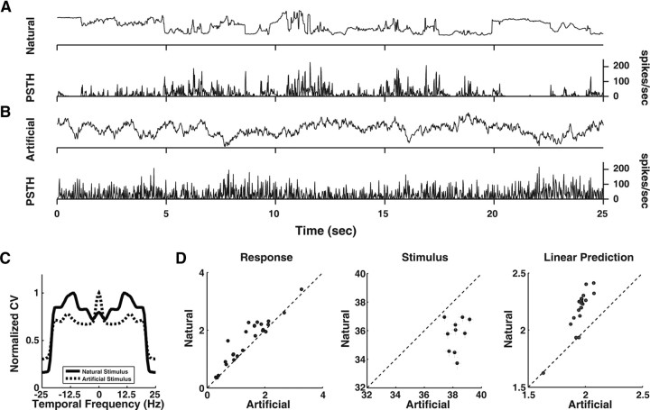
Comparison of spike train distance between natural and artificial stimuli. A, PSTH (bottom) of an example cell in response to the natural stimulus (top). The mean spike train distance between two randomly sampled response segments was 2.1. B, PSTH (bottom) of the same cell in response to the artificial stimulus (top), with a mean spike train distance of 1.6. C, The variability of power spectrum for the natural stimulus (solid) is different from that for the artificial stimulus (dotted). For each stimulus, the maximum CV was normalized to 1. D, Left, Spike train distance for the neural responses to natural versus artificial stimulus (n = 25, p < 10−4, Wilcoxon signed rank test). Middle, Stimulus distance for natural versus artificial stimulus (p < 0.005, Wilcoxon signed rank test). Each data point represents one set of natural and artificial stimulus. Right, Spike train distance for the predicted responses to natural versus artificial stimulus (p < 10−4, Wilcoxon signed rank test).
Analysis of spatiotemporal frequency properties of the RF.
To estimate the STRF, responses to the two-dimensional binary white noise were binned and reverse-correlated with the stimulus sequence (Cai et al., 1997; Reid et al., 1997). The two-dimensional space was radially collapsed to one-dimensional (Lesica et al., 2007). A two-dimensional Fast Fourier Transform (FFT) was applied to the STRF map (DeAngelis et al., 1993a) to obtain the spatiotemporal amplitude spectrum (STF map) in the quadrant of positive frequencies. A set of TF tuning curves, each corresponding to a different SF, were extracted from the STF map. We then identified a range of SFs at which the variance of the TF tuning curve was ≥0.08 of the maximum variance, and analyzed the TF tuning curves corresponding to these SFs. Each TF tuning curve was fitted with a gamma function (DeAngelis et al., 1993b; Cai et al., 1997) as follows:
 |
where f represents frequency, and A, fc, σ, and γ are free parameters. The peak TF was determined from the peak of the fitted tuning curve. The dependence of TF on SF can be estimated by the shift in TF peak with SF, which was the difference between the TF peaks corresponding to the lowest and the highest SF. To obtain the confidence interval for the shift in TF peak, we generated 100 jackknife data sets by each excluding a different 1% segment from the complete data set of the responses to the mapping stimulus (David et al., 2004). Each jackknife set was used to obtain an STRF map, and a corresponding STF map from which the shift in TF peak was estimated. From these jackknife sets, we computed the 95% confidence interval and the significance level for the shift in TF peak.
For each cell, we also extracted a one-dimensional spatial (temporal) profile from the STRF map by slicing through its peak parallel to the axis of space (time). We then applied FFT to transform each profile to SF (TF) tuning curve. We fitted each tuning curve with the gamma function, and the optimal SF (TF) for each cell can be estimated from the fitted curve. To obtain the ensemble STF map, we averaged the STF maps of all LGN neurons.
To estimate STRF from the responses to movie sequence of natural scenes (Lesica et al., 2007), we first computed a spike-triggered average (STA) vector by averaging all stimuli that elicited a spike (binned at 16.7 ms). We then corrected for the stimulus correlation by decorrelation with regularization (David and Gallant, 2005; Sharpee et al., 2006). To implement the regularization, we diagonalized the stimulus covariance matrix, and obtained a pseudoinverse of the matrix by choosing the eigenvectors below a cutoff point to multiply with the inverse of their corresponding eigenvalues. The cutoff point was chosen as 50% of the total number of eigenvectors, so that the high-frequency components above the cutoff point did not contribute to the inverse (other cutoff point, such as 30% or 80%, did not significantly influence the estimated STRF map for a model neuron and a trial set of neurons). The STRF was obtained by multiplying the STA by the pseudoinverse of the covariance matrix.
Analysis of stimulus statistics.
To estimate the spatiotemporal power spectrum of natural scenes, we randomly sampled 6900 segments of 620 ms movie from a natural scenes database (van Hateren and Ruderman, 1998) (spatial resolution, 32 × 32 pixels; frame rate, 50 Hz), and performed 2D FFT after applying a hamming window to each segment. We assumed that the visual angle of the image is ∼20 degrees. To quantify the variation in power spectrum across different movie segments, we calculated the coefficient of variation (CV) of the power spectrum, which is the SD divided by the mean. The SD of the power spectrum was estimated by jackknife method.
Optimal spatiotemporal filter.
Assuming that natural stimulus is transformed by a spatiotemporal filter and the filtered signal is delivered to a noisy channel with limited capacity, it is possible to predict a filter that is optimized to transmit maximum amount of information about natural stimulus with the constraint that the filtered signal is within the channel's dynamic range (van Hateren, 1992; Van Hateren, 1993).
The information rate I in the channel is as follows:
 |
where S(f) represents the spatiotemporal power spectrum of the natural stimulus, K(f) is the spatiotemporal power spectrum of the filter, and Ni(f) and Nc(f) is the power spectrum of input noise and channel noise, respectively.
The dynamic range of the channel R is as follows:
 |
Given a certain signal-to-noise ratio, the method of Lagrange multipliers is used to maximize the information rate I subject to the constraint that the response is within the channel's dynamic range (i.e., R is a constant). By introducing a new variable λ called a Lagrange multiplier, we require the following:
 |
which leads to the following:
 |
We find K(f) by choosing the value of λ so that the response range R is a constant (van Hateren, 1992; Van Hateren, 1993).
While the above method is used to compute the optimal transfer function for individual cell, it can also predict the optimal SF and optimal TF for a population of cells. Assuming that
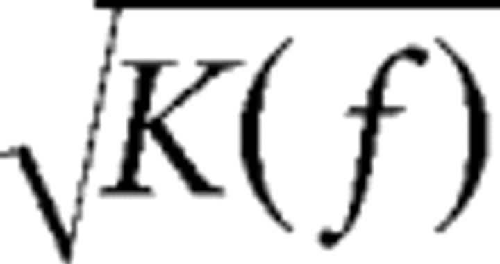 |
represents the probability distribution of optimal spatiotemporal frequency for the population and the gain is the same for each cell, based on the same assumption that early visual system aims at maximizing information transfer through noisy channels, the probability distribution of optimal SF and optimal TF for the population can be estimated using the above equation that solved for K(f).
Spike train distance.
We estimated neural discrimination using spike train distance. For the two types of spatially uniform temporal stimuli (natural vs artificial stimulus) that matched in the mean power spectrum but differed in the variability of spectrum, we averaged the responses over trials and binned the histogram at 16.7 ms. To remove the effect of mean firing rate on the value of spike train distance, we normalized the histogram by its mean rate. We then randomly sampled two segments (300 ms) of the normalized responses and calculated the Euclidean distance between them:
 |
where A(t) and B(t) represent the two segments of responses. The random sampling was repeated 4000 times, and an average spike train distance was calculated. We also computed spike train distance for the responses predicted by the STRF (Dan et al., 1996).
Stimulus distance.
To compute stimulus distance, the natural stimulus (or the artificial stimulus) was first normalized to zero mean. We then sampled two segments (300 ms) of the normalized stimuli, and used the same equation for spike train distance to compute the stimulus distance. The distance was averaged over 4000 repeats of random sampling.
Results
We made single-unit recordings from 140 LGN neurons in the anesthetized adult cat. Binary white noise stimuli were used to map the STRF (Reid et al., 1997), and contrast reversal gratings were used to classify the cells as X or Y (Hochstein and Shapley, 1976).
Inseparability of spatial and temporal frequency tuning in LGN
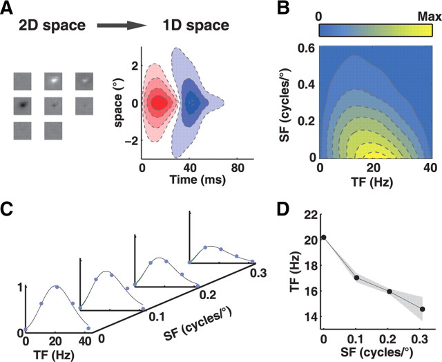
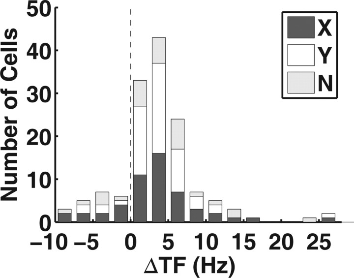
The STRF of LGN neurons was estimated by cross-correlating the peristimulus time histogram (PSTH) and the sequence of the two-dimensional white noise. Figure 1A shows the STRF map of an ON-center LGN neuron (left), and the map collapsed along the radius of space (right), with red and blue pixels representing regions activated by light and dark stimulus, respectively. To examine the SF and TF tuning of the neuron, we performed 2D FFT on the STRF map (DeAngelis et al., 1993a). Figure 1B shows a map of the amplitude spectrum in the joint spatiotemporal frequency domain (STF map), in which the intensity of yellow pixels represented the level of activity at the corresponding spatiotemporal frequency. The STF map exhibited a slanted feature, indicating dependence between SF and TF. When we plotted the STF map as a set of TF curves (Fig. 1C), each for a given SF, we found that the TF peaks shifted from low to high frequency as SF changed from high to low frequency (Fig. 1D). To quantify the degree of shift in TF peak, we calculated the difference between TF peaks corresponding to the lowest and the highest SF within a significant region of the STF map (Materials and Methods). For a population of 140 neurons examined, the shift in TF peaks was 3.6 ± 0.5 Hz (Fig. 2, mean ± SEM, p < 10−5, Wilcoxon signed rank test), and 78.6% of the neurons showed significant increase in the TF peak as the SF decreased (Materials and Methods). The result indicates that higher TF is associated with lower SF, and vice versa. Thus, the RF of individual LGN neurons exhibited inseparability of spatial frequency and temporal frequency tuning.
Figure 1.
Spatiotemporal frequency tuning characteristics of LGN neurons. A, Left, STRF of an example LGN neuron. Right, A map obtained by radially collapsing the one on the left. Red and blue represent regions activated by light and dark stimulus, respectively. B, STF map of the neuron, obtained by applying FFT on the radially collapsed STRF map. The intensity of yellow pixels represents the level of activity at the corresponding spatiotemporal frequency. C, A set of TF tuning curves extracted from the STF map in B. D, The peaks of the TF tuning curves are plotted against the corresponding SFs. Shaded area indicates 95% confidence interval.
Figure 2.
Distribution of the shift in TF peak. The TF shift is the difference between the TF peak for the lowest SF and that for the highest SF. Positive shift means that TF increases as SF decreases. Dark bars, X cells (n = 52). White bars, Y cells (n = 58). Gray bars, Cells that were not classified (n = 30).
We further estimated the optimal SF (SFo) and optimal TF (TFo) for each neuron, to examine the relationship between SF and TF selectivity over the population. We extracted a one-dimensional spatial (temporal) profile from the STRF map by slicing through the peak parallel to the axis of space (time) (Fig. 3A), and applied Fourier transform on the spatial and temporal profile to obtain an SF tuning and a TF tuning curve, respectively (Fig. 3B). The SFo or TFo for each cell was determined by fitting the tuning curve with a gamma function (Materials and Methods). When we plotted the TFo against the SFo for the population of neurons (Fig. 3C), we found that the two parameters exhibited a negative correlation (r = −0.25, p < 0.005), indicating neurons preferring higher (lower) TF were tuned to lower (higher) SF. Thus, SF and TF selectivity are negatively correlated with each other in LGN, at the level of population as well as single RF. When we averaged the STF maps over the population, we found that the ensemble STF map (eSTF) also exhibited a slanted feature (Fig. 3D), which can be accounted for by the inseparability of SF and TF tuning at single cell level (Figs. 1, 2) and the correlation between SF and TF at population level (Fig. 3C).
Figure 3.
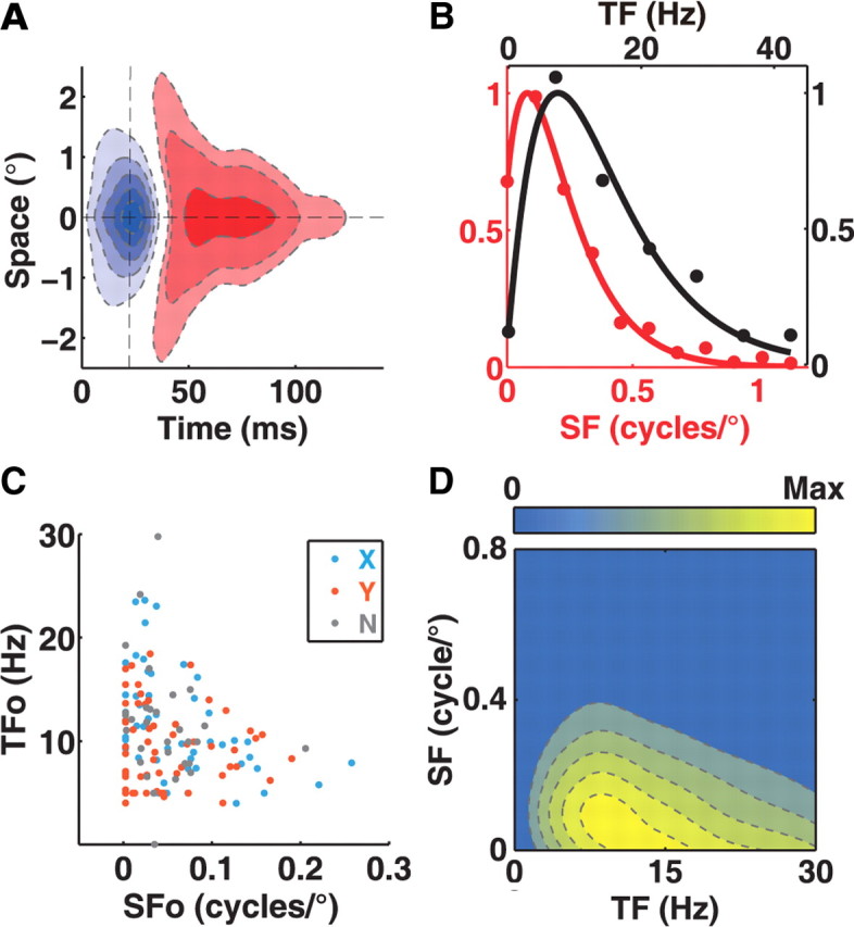
SF and TF selectivity for a population of LGN neurons. A, A spatial (temporal) profile can be extracted from the STRF map along the vertical (horizontal) dashed line that passed through the peak of the STRF map. B, SF (red) and TF (black) tuning curve was obtained by applying FFT on the spatial and temporal profile, respectively. C, Joint distribution of optimal SF and optimal TF for a population of LGN neurons (n = 140, r = −0.25, p < 0.005). Cyan, X cells. Red, Y cells. Gray, cells that were not classified. D, Ensemble STF map for the population of neurons.
RF in the early visual pathway can change adaptively with the input stimulus (David et al., 2004; Sharpee et al., 2006; Lesica et al., 2007). To examine whether such inseparable STF tuning can be observed under stimulation of natural stimuli, we compared STRFs mapped with noise and movie stimuli for a subset of cells (n = 18). Figure 4A shows the results for an example cell mapped with noise (upper) and movie (lower) stimuli. The correlation coefficient (CC) between the two STRF maps was 0.92, and the CC between the two STF maps was 0.96. For 18 cells examined, the mean CC between STF maps measured with noise and movie was 0.91 ± 0.02 (mean ± SEM) (Fig. 4B), and the ensemble STF map under movie stimulation also exhibited a slanted feature (Fig. 4C). This indicates that the inseparable spatiotemporal frequency tunings of LGN neurons measured with noise and natural stimuli were comparable.
Figure 4.

Comparison of the STF maps measured with noise and movie stimuli. A, Top, STRF (left) and STF map (right) for an example cell estimated using noise stimuli. Bottom, STRF (left) and STF map (right) for the same cell estimated using movie stimuli. B, Distribution of the CC between STF maps measured with noise and movie stimuli for 18 neurons. C, Ensemble STF map of the 18 cells measured with movie stimuli.
LGN spatiotemporal frequency tuning resembles the optimal filter
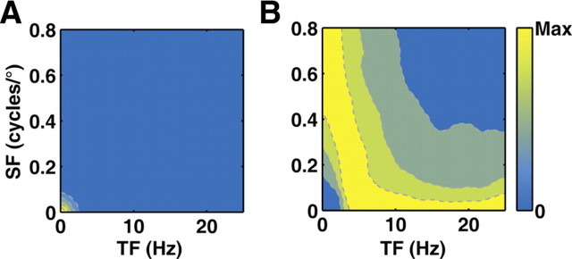
Assuming that the early visual processing reduces stimulus redundancy at high signal-to-noise ratio (SNR) and increases redundancy at low SNR, previous theoretical studies predicted an optimal spatiotemporal filter that maximizes the stimulus information transmitted through a noisy channel of limited capacity (van Hateren, 1992; Van Hateren, 1993; Li, 1996; Dong and Atick, 1997). We applied a similar method to compute the spatiotemporal frequency tuning of the optimal filter using the amplitude spectrum of natural scenes (Fig. 5A) (Materials and Methods). For a range of SNRs, we found that the optimal filter exhibited inseparable spatiotemporal frequency tuning, in which the preferred SF is negatively correlated with the preferred TF (Fig. 5B). As this method of optimization can be extended to derive the optimal SF and optimal TF for a population of filters (Materials and Methods), Figure 5B also represents the joint distribution of SF and TF selectivity for ensemble filters that are optimized to transmit information of natural scenes. Thus, the inseparable STF tuning of LGN neurons resembles the feature of the optimal spatiotemporal filter, which suggests that LGN STF tuning may serve as an efficient strategy to maximize the information carried by the neural responses about natural scenes. Of course, there are important limitations of the theory, since the optimal filters are derived within a linear framework, based on specific assumptions on the Gaussian statistics of the input signals and on the sources of noise (Atick, 1992; van Hateren, 1992). Nevertheless, it provides a useful approximation for understanding how the spatiotemporal RF properties of LGN neurons contribute to optimal coding of natural stimuli.
Figure 5.
Optimal filters exhibit inseparable spatiotemporal frequency tuning. A, Amplitude spectrum of natural scenes. B, Optimal filter obtained at SNR of 4. The map also represents the distribution of preferred SF and preferred TF for a population of optimal filters.
LGN frequency tuning matches the variation of natural power spectrum
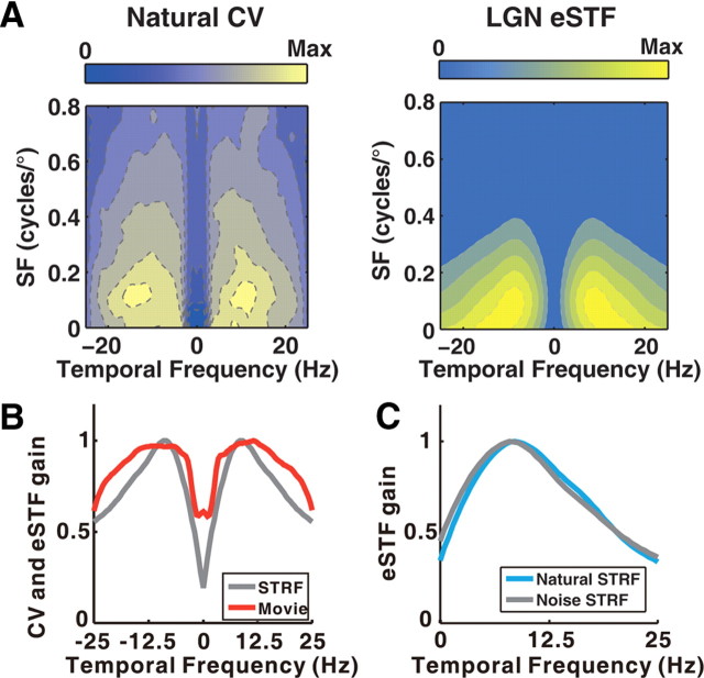
In addition to the inseparability of SF and TF tuning, another noticeable feature in the ensemble STF map is the low-pass SF tuning and the bandpass TF tuning (Fig. 3D). Since this feature was not observed in the optimal spatiotemporal filter computed at a range of SNRs, we further explored whether it is related to the statistics of natural scenes. In particular, we speculated that the power at specific range of frequencies may vary among different natural scenes, similar to that in natural sounds (Woolley et al., 2005), and a possible coding strategy of LGN neurons is to tune to the frequency components that are relevant for distinguishing one scene from another. To examine such a possibility, we analyzed the variation of natural power spectrum by calculating the coefficient of variation (CV) across the spectra of thousands of natural scenes movies (Materials and Methods). Higher CV values were found for low SF and intermediate TF components (Fig. 6A, left), indicating that the power at these frequencies is highly variable across different movies. Interestingly, the shape of CV map largely resembled that of the eSTF map of LGN neurons (Fig. 6A, right), with a CC of 0.79. Because the SF in the CV map is scalable depending on the visual angle of the natural images, we examined the relationship between the CV map and the eSTF map by collapsing both maps into the TF domain (Fig. 6B). The CV of natural temporal power spectrum (Fig. 6B, red) is high ∼10 Hz, and its peak overlaps with the peak of LGN TF tuning (Fig. 6B, gray) mapped with noise and with movie (Fig. 6C, cyan). Clearly, the frequency tuning of ensemble LGN neurons selectively amplifies the range of frequencies in which power varies most among different natural scenes.
Figure 6.
LGN frequency tuning versus the variation of natural power spectrum. A, Left, CV of natural power spectrum. Right, ensemble STF map of 140 LGN neurons measured with noise stimuli. In the eSTF map, the amplitude in the negative TFs was a mirror image of that in the positive TFs. B, TF tuning of ensemble LGN neurons (gray) versus the CV of temporal power spectrum for natural scenes (red). Both curves are normalized to have peak amplitude of 1. C, For a subset of LGN neurons (n = 18), the ensemble TF tuning measured with movie stimuli (cyan) was similar to that measured with noise stimuli (gray).
Better neural discrimination for natural than for artificial stimuli
Given the similarity between LGN temporal frequency tuning and the CV of natural temporal power spectrum (Fig. 6B), we wondered whether it can facilitate neural discrimination for natural stimuli. We tested this hypothesis by comparing the neural responses to natural and artificial stimuli, in which the mean power spectrum was similar as natural but the variability of the spectrum did not match the LGN temporal frequency tuning (Materials and Methods) (Fig. 7C). For the example cell in Figure 7, A and B, the mean spike train distance between two randomly sampled response segments was 2.1 for the natural stimulus (Fig. 7A, top) and 1.6 for the artificial stimulus (Fig. 7B, top). Over the population of neurons, the spike train distance was significantly larger for the natural stimulus than for the artificial stimulus (n = 25, p < 10−4, Wilcoxon signed rank test) (Fig. 7D, left), despite the fact that the distance for two segments of natural stimulus was smaller than that for two segments of artificial stimulus (p < 0.005, Wilcoxon signed rank test) (Fig. 7D, middle). This indicates that LGN RF is able to transform the input signals in such a way that neural discrimination is enhanced for natural stimuli. When we analyzed the predicted responses obtained by convolving the STRF with the stimuli, we found that the spike train distance of the predicted response was also larger for natural than for artificial stimulus (p < 10−4, Wilcoxon signed rank test) (Fig. 7D, right), indicating that the enhanced neural discrimination can be accounted for by the linear STRF properties. Thus, the match between the LGN temporal frequency tuning and the variation of natural temporal power spectrum may facilitate neural discrimination of different natural stimuli.
Discussion
In the present study, we have shown that LGN neurons exhibit spatiotemporal coupling in the frequency domain at single cell as well as at population level. The inseparability of spatial and temporal frequency tuning is consistent with the predicted spatiotemporal filter optimized for information transmission of natural scenes, and is similar to the feature of variation of natural power spectrum. Such spatiotemporal frequency tuning assists in the processing of natural scenes through redundancy reduction and better neural discrimination of natural stimuli.
Relationship to the decorrelation theory and response equalization hypothesis
Theory based on efficient coding hypothesis proposed that the early visual system serves to decorrelate the incoming signals that contain redundant information (Atick, 1992). Using the second-order statistics of natural scenes (Field, 1987), the theory correctly predicted that the gain of the neural filter should change with frequency so that the output response to natural scenes has a flat spectrum over a range of frequencies (Atick, 1992; Dong and Atick, 1995; Dan et al., 1996).
However, the decorrelation theory used the second-order statistics to capture all information about natural scenes by assuming that the power density distribution is Gaussian with zero-mean for each frequency (Atick, 1992). For natural scenes, the mean of power density in each frequency channel is always non-negative instead of zero, and the variation of power in each frequency channel is unlikely to be always proportional to the mean power in the corresponding channel. Since the variation of power makes the power density unpredictable, more information is contained in those frequency channels in which the power varies more. Thus, the match between LGN frequency tuning and the CV of natural power spectrum is an efficient strategy for dense sampling the range of frequencies that contain more information.
Another theory addressing the flattening of output spectrum is the response equalization hypothesis (Field, 1987; Graham et al., 2006). This theory states that, neurons preferring higher spatial frequency exhibit higher gain, so that each neuron responds with the same average activity to natural scenes. Previous study in the retina (Croner and Kaplan, 1995) showed that the peak sensitivity of retinal ganglion cell is inversely proportional to the spatial area, which leads to lower gain for cells with larger RF (or lower spatial frequency). For cortical neurons, the spatial frequency bandwidths were shown to increase with optimal frequency, which results in increased gain in proportion to spatial frequency (De Valois et al., 1982). Since SF and TF selectivity are negatively correlated in LGN (Fig. 3C), at low TF, LGN cells preferring high SF will have higher gain relative to those preferring low SF. Therefore, the negative correlation between optimal SF and optimal TF over the LGN population can also serve as a potential mechanism to implement response equalization.
Higher-order statistics
In the present study, we have examined the natural power spectrum and the variation of the spectrum. Previous studies showed that, higher-order statistical regularities of natural images, which may arise from edges and lines, are more perceptually important (Thomson, 1999; Simoncelli and Olshausen, 2001). Using different algorithms that belong to the class of independent components analyses, several theoretical studies predicted linear filters that maximally reduce the higher-order redundancy in natural stimuli, and these filters largely resembled the structure of simple cells in the visual cortex (Olshausen and Field, 1996; Bell and Sejnowski, 1997; van Hateren and Ruderman, 1998). Although the analysis of higher-order structure remains a computational challenge, further investigation on the relationship between RF and higher-order statistics is required to reveal the coding strategy of the visual system.
Footnotes
This work was supported by grants from Knowledge Innovation Project from the Chinese Academy of Sciences KSCX2-YW-R-29, the National Basic Research Program in China (973 Program 2006CB806600), the Hundred Talent Program of the Chinese Academy of Sciences (2008–2010), and the Science and Technology of Shanghai Municipality (06dj14010). We thank Christoph Kayser and Nicholas Lesica for kindly providing the natural scene movies used for mapping STRF. We thank Si Wu, Libo Ma, Zhe Chen, Hao Li, Liang She, and Xiaodong Chen for helpful discussion. We thank Peipei Li, Huiyuan Zhong, and Weiqi Xu for technical assistance.
References
- Atick JJ. Could information theory provide an ecological theory of sensory processing? Network. 1992;3:213–251. doi: 10.3109/0954898X.2011.638888. [DOI] [PubMed] [Google Scholar]
- Barlow HB. Possible principles underlying the transformation of sensory messages. In: Rosenblith WA, editor. Sensory communication. Cambridge, MA: MIT; 1961. pp. 217–234. [Google Scholar]
- Bell AJ, Sejnowski TJ. The “independent components” of natural scenes are edge filters. Vision Res. 1997;37:3327–3338. doi: 10.1016/s0042-6989(97)00121-1. [DOI] [PMC free article] [PubMed] [Google Scholar]
- Butts DA, Weng C, Jin J, Yeh CI, Lesica NA, Alonso JM, Stanley GB. Temporal precision in the neural code and the timescales of natural vision. Nature. 2007;449:92–95. doi: 10.1038/nature06105. [DOI] [PubMed] [Google Scholar]
- Cai D, DeAngelis GC, Freeman RD. Spatiotemporal receptive field organization in the lateral geniculate nucleus of cats and kittens. J Neurophysiol. 1997;78:1045–1061. doi: 10.1152/jn.1997.78.2.1045. [DOI] [PubMed] [Google Scholar]
- Croner LJ, Kaplan E. Receptive fields of P and M ganglion cells across the primate retina. Vision Res. 1995;35:7–24. doi: 10.1016/0042-6989(94)e0066-t. [DOI] [PubMed] [Google Scholar]
- Dan Y, Atick JJ, Reid RC. Efficient coding of natural scenes in the lateral geniculate nucleus: experimental test of a computational theory. J Neurosci. 1996;16:3351–3362. doi: 10.1523/JNEUROSCI.16-10-03351.1996. [DOI] [PMC free article] [PubMed] [Google Scholar]
- David SV, Gallant JL. Predicting neuronal responses during natural vision. Network. 2005;16:239–260. doi: 10.1080/09548980500464030. [DOI] [PubMed] [Google Scholar]
- David SV, Vinje WE, Gallant JL. Natural stimulus statistics alter the receptive field structure of v1 neurons. J Neurosci. 2004;24:6991–7006. doi: 10.1523/JNEUROSCI.1422-04.2004. [DOI] [PMC free article] [PubMed] [Google Scholar]
- DeAngelis GC, Ohzawa I, Freeman RD. Spatiotemporal organization of simple-cell receptive fields in the cat's striate cortex. I. General characteristics and postnatal development. J Neurophysiol. 1993a;69:1091–1117. doi: 10.1152/jn.1993.69.4.1091. [DOI] [PubMed] [Google Scholar]
- DeAngelis GC, Ohzawa I, Freeman RD. Spatiotemporal organization of simple-cell receptive fields in the cat's striate cortex. II. Linearity of temporal and spatial summation. J Neurophysiol. 1993b;69:1118–1135. doi: 10.1152/jn.1993.69.4.1118. [DOI] [PubMed] [Google Scholar]
- Derrington AM, Lennie P. Spatial and temporal contrast sensitivities of neurones in lateral geniculate nucleus of macaque. J Physiol. 1984;357:219–240. doi: 10.1113/jphysiol.1984.sp015498. [DOI] [PMC free article] [PubMed] [Google Scholar]
- De Valois RL, Albrecht DG, Thorell LG. Spatial frequency selectivity of cells in macaque visual cortex. Vision Res. 1982;22:545–559. doi: 10.1016/0042-6989(82)90113-4. [DOI] [PubMed] [Google Scholar]
- Dong DW, Atick JJ. Temporal decorrelation: a theory of lagged and nonlagged responses in the lateral geniculate nucleus. Network. 1995;6:159–178. [Google Scholar]
- Dong DW, Atick JJ. Spatiotemporal coupling and scaling of natural images and human visual sensitivities. Cambridge, MA: MIT; 1997. [Google Scholar]
- Enroth-Cugell C, Robson JG, Schweitzer-Tong DE, Watson AB. Spatio-temporal interactions in cat retinal ganglion cells showing linear spatial summation. J Physiol. 1983;341:279–307. doi: 10.1113/jphysiol.1983.sp014806. [DOI] [PMC free article] [PubMed] [Google Scholar]
- Felsen G, Touryan J, Han F, Dan Y. Cortical sensitivity to visual features in natural scenes. PLoS Biol. 2005;3:e342. doi: 10.1371/journal.pbio.0030342. [DOI] [PMC free article] [PubMed] [Google Scholar]
- Field DJ. Relations between the statistics of natural images and the response properties of cortical cells. J Opt Soc Am A. 1987;4:2379–2394. doi: 10.1364/josaa.4.002379. [DOI] [PubMed] [Google Scholar]
- Frishman LJ, Freeman AW, Troy JB, Schweitzer-Tong DE, Enroth-Cugell C. Spatiotemporal frequency responses of cat retinal ganglion cells. J Gen Physiol. 1987;89:599–628. doi: 10.1085/jgp.89.4.599. [DOI] [PMC free article] [PubMed] [Google Scholar]
- Graham DJ, Chandler DM, Field DJ. Can the theory of “whitening” explain the center-surround properties of retinal ganglion cell receptive fields? Vision Res. 2006;46:2901–2913. doi: 10.1016/j.visres.2006.03.008. [DOI] [PMC free article] [PubMed] [Google Scholar]
- Hochstein S, Shapley RM. Quantitative analysis of retinal ganglion cell classifications. J Physiol. 1976;262:237–264. doi: 10.1113/jphysiol.1976.sp011594. [DOI] [PMC free article] [PubMed] [Google Scholar]
- Hsu A, Woolley SM, Fremouw TE, Theunissen FE. Modulation power and phase spectrum of natural sounds enhance neural encoding performed by single auditory neurons. J Neurosci. 2004;24:9201–9211. doi: 10.1523/JNEUROSCI.2449-04.2004. [DOI] [PMC free article] [PubMed] [Google Scholar]
- Kayser C, Einhauser W, Konig P. Temporal correlations of orientations in natural scenes. Neurocomputing. 2003;52:117–123. [Google Scholar]
- Lesica NA, Jin J, Weng C, Yeh CI, Butts DA, Stanley GB, Alonso JM. Adaptation to stimulus contrast and correlations during natural visual stimulation. Neuron. 2007;55:479–491. doi: 10.1016/j.neuron.2007.07.013. [DOI] [PMC free article] [PubMed] [Google Scholar]
- Li Z. A theory of the visual motion coding in the primary visual cortex. Neural Comput. 1996;8:705–730. doi: 10.1162/neco.1996.8.4.705. [DOI] [PubMed] [Google Scholar]
- Olshausen BA, Field DJ. Emergence of simple-cell receptive field properties by learning a sparse code for natural images. Nature. 1996;381:607–609. doi: 10.1038/381607a0. [DOI] [PubMed] [Google Scholar]
- Reid RC, Victor JD, Shapley RM. The use of m-sequences in the analysis of visual neurons: linear receptive field properties. Vis Neurosci. 1997;14:1015–1027. doi: 10.1017/s0952523800011743. [DOI] [PubMed] [Google Scholar]
- Sharpee TO, Sugihara H, Kurgansky AV, Rebrik SP, Stryker MP, Miller KD. Adaptive filtering enhances information transmission in visual cortex. Nature. 2006;439:936–942. doi: 10.1038/nature04519. [DOI] [PMC free article] [PubMed] [Google Scholar]
- Simoncelli EP. Vision and the statistics of the visual environment. Curr Opin Neurobiol. 2003;13:144–149. doi: 10.1016/s0959-4388(03)00047-3. [DOI] [PubMed] [Google Scholar]
- Simoncelli EP, Olshausen BA. Natural image statistics and neural representation. Annu Rev Neurosci. 2001;24:1193–1216. doi: 10.1146/annurev.neuro.24.1.1193. [DOI] [PubMed] [Google Scholar]
- Thomson MG. Higher-order structure in natural scenes. J Opt Soc Am A. 1999;16:1549–1553. [Google Scholar]
- Troy JB. Spatial contrast sensitivities of X and Y type neurones in the cat's dorsal lateral geniculate nucleus. J Physiol. 1983;344:399–417. doi: 10.1113/jphysiol.1983.sp014948. [DOI] [PMC free article] [PubMed] [Google Scholar]
- van Hateren JH. A theory of maximizing sensory information. Biol Cybern. 1992;68:23–29. doi: 10.1007/BF00203134. [DOI] [PubMed] [Google Scholar]
- Van Hateren JH. Spatiotemporal contrast sensitivity of early vision. Vision Res. 1993;33:257–267. doi: 10.1016/0042-6989(93)90163-q. [DOI] [PubMed] [Google Scholar]
- van Hateren JH, Ruderman DL. Independent component analysis of natural image sequences yields spatio-temporal filters similar to simple cells in primary visual cortex. Proc Biol Sci. 1998;265:2315–2320. doi: 10.1098/rspb.1998.0577. [DOI] [PMC free article] [PubMed] [Google Scholar]
- van Hateren JH, Rüttiger L, Sun H, Lee BB. Processing of natural temporal stimuli by macaque retinal ganglion cells. J Neurosci. 2002;22:9945–9960. doi: 10.1523/JNEUROSCI.22-22-09945.2002. [DOI] [PMC free article] [PubMed] [Google Scholar]
- Woolley SM, Fremouw TE, Hsu A, Theunissen FE. Tuning for spectro-temporal modulations as a mechanism for auditory discrimination of natural sounds. Nat Neurosci. 2005;8:1371–1379. doi: 10.1038/nn1536. [DOI] [PubMed] [Google Scholar]
- Zhaoping L. Theoretical understanding of the early visual processes by data compression and data selection. Network. 2006;17:301–334. doi: 10.1080/09548980600931995. [DOI] [PubMed] [Google Scholar]


