

Abstract
Perceiving the three-dimensional (3D) properties of the environment relies on the brain bringing together ambiguous cues (e.g., binocular disparity, shading, texture) with information gained from short- and long-term experience. Perceptual aftereffects, in which the perception of an ambiguous 3D stimulus is biased away from the shape of a previously viewed stimulus, provide a sensitive means of probing this process, yet little is known about their neural basis. Here, we investigate 3D aftereffects using psychophysical and functional MRI (fMRI) adaptation paradigms to gain insight into the cortical circuits that mediate the perceptual interpretation of ambiguous depth signals. Using two classic bistable stimuli (Mach card, kinetic depth effect), we test aftereffects produced by 3D shapes defined by binocular (disparity) or monocular (texture, shading) depth cues. We show that the processing of ambiguous 3D stimuli in dorsal visual cortical areas (V3B/KO, V7) and posterior parietal regions is modulated by adaptation in line with perceptual aftereffects. Similar behavioral and fMRI adaptation effects for the two types of bistable stimuli suggest common neural substrates for depth aftereffects independent of the inducing depth cues (disparity, texture, shading). In line with current thinking about the role of adaptation in sensory optimization, our findings provide evidence that estimation of 3D shape in dorsal cortical areas takes account of the adaptive context to resolve depth ambiguity and interpret 3D structure.
Keywords: ambiguous perception, bistability, fMRI adaptation, depth perception, psychophysics, vision
Introduction
Perceiving the three-dimensional (3D) structure of the world is a fundamental visual ability, supporting interaction with people and objects around us. To estimate depth, the brain relies on signals whose interpretation is ambiguous: the inverse mapping from retina to world is ill-posed and different cues (e.g., binocular disparity, perspective, texture) may provide conflicting information. Well known ambiguous figures, such as the Necker cube, illustrate the brain's dilemma: different depth configurations are compatible with the same sensory input, resulting in alternating interpretations. Understanding the processing involved in translating ambiguous depth signals into a perceptual estimate of 3D structure remains an open challenge.
A widely used behavioral technique for probing the relationship between sensory signals (e.g., disparity) and their interpretation (e.g., 3D shape) is to exploit the adaptive properties of the visual system. For instance, prolonged viewing of disparity-defined surfaces causes a shift in the perception of a subsequently presented surface (Kohler and Emery, 1947; Bergman and Gibson, 1959; Blakemore and Julesz, 1971; Berends et al., 2005; Taya et al., 2005; Knapen and van Ee, 2006). Despite considerable interest in the role of adaptation in perceptual estimation (Clifford et al., 2007), the cortical circuits engaged by these aftereffects remain unknown. Here, we combine bistable stimuli with psychophysical and functional MRI (fMRI) adaptation paradigms to investigate the brain regions involved in interpreting depth structure when sensory input remains ambiguous but 3D shape perception is guided by adaptation.
We used two classic bistable stimuli: (1) the Mach card (Mach, 1886) (see Fig. 1A) that gives rise to two competing depth percepts: either “convex” (like viewing the covers of a book) or “concave” (like viewing the internal pages of a book); (2) the kinetic depth effect (KDE) (Wallach and O'Connell, 1953) in which observers perceive either the interior (convex) or exterior (concave) surface of a rotating half-cylinder. By adding binocular disparity to the Mach card (see Fig. 1B) or shading and texture to the KDE cylinder (see Fig. 1C), we disambiguated these bistable stimuli. We investigated how adapting to a convex or concave stimulus affected both the perceptual and fMRI responses to a subsequently presented ambiguous stimulus.
Figure 1.

Stimuli and behavioral data. A, A bistable Mach card stimulus. B, A disparity-defined Mach card. When viewed through red-green glasses (left eye red) the stimulus appears concave. The vertical lines flanking the fixation marker were provided to assist correct eye vergence. C, Illustrations of the KDE stimulus. The stimulus rotated around its vertical axis to depict the exterior or interior surface of a cylinder. Texture and shading cues disambiguated the stimulus (left, center), while the ambiguous stimulus was a shuffled version of the convex and concave stimuli. The arrows depict rotation in depth. D, An example psychometric curve showing the proportion of trials on which the observer interpreted the probe Mach card stimulus as concave. Data are shown for the concave adaptor (blue squares), the convex adaptor (red triangles), and in the absence of an adaptor (baseline: black circles). E, F, Group behavioral data (means with error bars depicting bootstrapped 68% confidence intervals) for the Mach card (E) and the KDE stimuli (F). Results are shown for three different types of probe stimuli (convex, zero, concave) following different types of adaptation (convex, baseline, concave).
We observed repulsion aftereffects whereby bistable stimuli were perceived as concave more often following adaptation to a convex shape and convex more frequently following exposure to a concave shape. Using an event-related fMRI adaptation paradigm (Huk et al., 2001; Boynton and Finney, 2003; Fang et al., 2005), we investigated the neural basis of this effect, studying fMRI responses to pairs of adaptor and probe stimuli that could differ in their depth structure and/or perceptual interpretation. We tested for rebound effects (i.e., higher responses for stimuli perceived to have a different, rather than same, 3D structure) to reveal neural populations representing the perceived 3D shape of bistable stimuli. By relating behavioral repulsion and fMRI rebound results, we provide evidence that dorsal visual cortical areas (V3B/KO, V7) and posterior parietal regions play an important role in the adaptive estimation and perception of ambiguous 3D shape from different depth cues.
Materials and Methods
Observers
Six adults participated in the Mach card experiment, three in the KDE experiment and seven in the control experiments. Mean age was 26 (range 22–33). All observers had normal or corrected-to-normal vision. The study was approved by the local ethics committee and participants gave written informed consent.
Stimuli
The Mach card stimulus consisted of two abutting parallelograms (see Fig. 1A) with internal acute angles of 60°. The stimulus subtended 3.7 × 5.1°. To disambiguate 3D shape, disparity was added (range −6.2 to 6.6 arcmin) to the contours to create a pair of slanted planes that approached or receded with disparity-defined dihedral angles ranging from −40° (convex) to +40° (concave). Nonius lines were presented to aid correct vergence. Stimuli were surrounded by an array of open squares (0.6°) positioned in the fixation plane to aid stabilized fixation. The KDE stimulus consisted of an array of 375 gray dots (see Fig. 1B) and subtended 2.6 × 5.4°. For unambiguous stimuli, the motion and size of the dots was determined by perspective projection of the 1.5 cm radius cylinder and dot luminance was determined using a Blinn–Phong shading model [psychophysical experiments revealed this combination of cues to be effective in disambiguating motion, contrasting with the single cue manipulations reported to be ineffective (Nawrot and Blake, 1991)]. For ambiguous stimuli, orthographic projection was used, dot luminance was determined as the shuffled values from the unambiguous stimuli and angular velocity was varied sinusoidally to a peak of 31.8°/s. Dot number, size and luminance were very closely matched between conditions. To minimize motion aftereffects, cylinder rotation (clockwise or anticlockwise) was alternated 10 or 11 times (randomized) during the 4 s presentation.
Psychophysical experiments
For the Mach card experiment, observers (n = 6) participated in three experiments in the lab before scanning. First, we assessed the rate of perceptual reversals for the ambiguous Mach card stimulus viewed continuously (3 blocks of 3 min each separated by 16 s). Observers maintained central fixation and reported whether they perceived a convex or concave shape. Second, to provide nonadapted baseline measures, we tested shape discrimination (convex or concave) for a range of Mach card stimuli rendered with disparity (dihedral angles = 0, ± [5, 10, 15, 20, 30, 40]°) and presented for 400 ms. Third, we assessed the effect of adaptation on the interpretation of a probe stimulus. A single trial is depicted in supplemental Figure S1C, available at www.jneurosci.org as supplemental material: a convex (+40°) or concave (−40°) adaptor (4 s) was followed by a blank fixation interval (1.4 s), a probe stimulus (400 ms) and finally another fixation interval (2 s). Convex and concave adaptors were presented on separate runs. Observers performed two tasks during each trial. During the adaption phase, observers detected a letter Y among Xs presented at a rate of one character every 250 ms (attentional task). Second, observers indicated the 3D shape of the adaptor and the probe during the fixation intervals following stimulus presentation (shape task). A similar design was used for the KDE experiment. The attentional task during the KDE adaptation phase required observers to attend to the rotation direction of the cylinder and report whether it rotated to the left or the right immediately before the disappearance of the adaptor. The 3D shape task (convex or concave) was the same as for the Mach card experiment.
Imaging: scanner and peripheral equipment
Data were collected at the Birmingham University Imaging Centre using a 3 Tesla Philips MRI scanner with an 8-channel head coil. fMRI data were recorded with an echo-planar imaging sequence [echo time (TE) 35 ms; repetition time (TR) 2000 ms, voxel size 2.5 × 2.5 × 3 mm, 33 slices] for the localizer scans and (TE: 35 ms, TR: 1300 ms, voxel size 2.5 × 2.5 × 4.5–5 mm, 21 slices) for the fMRI adaptation and control experiments. A high resolution anatomical scan (1 mm3) was also acquired for each participant.
To achieve stereoscopic presentation, we used a pair of video projectors (JVC; D-ILA SX21) that contained separate spectral interference filters (INFITEC). The images from the two projectors were optically combined using a beam-splitter before being passed through a wave guide into the scanner room. The interference filters produce negligible overlap between the emission spectra for each projector with the result that there is extremely little cross talk. Stimuli were back-projected onto a screen inside the bore of the magnet and viewed via a mirror above the observers' heads. The viewing distance was 65 cm and stimuli subtended 3.7 × 5.1° (Mach card) and 2.6 × 5.4° (KDE).
fMRI adaptation experiments
The protocol for the fMRI adaptation experiment was identical to the psychophysical testing and yielded similar behavioral results (supplemental Fig. S1D, available at www.jneurosci.org as supplemental material). We measured fMRI responses for three different adaptor stimuli: convex (+40°), concave (−40°) or a flat two-dimensional control stimulus (supplemental Fig. S5A, available at www.jneurosci.org as supplemental material). For each adaptor, we examined the fMRI response to four different probe stimuli: convex, concave, zero disparity and a probe with disparity equal to the subject's point of subjective equality (determined before scanning). A similar procedure was used for the KDE experiment.
fMRI data analysis
For each individual observer, anatomical scans were transformed into Talairach space and inflated and flattened surfaces of both hemispheres were rendered using BrainVoyager QX (BrainInnovation B.V.). All functional runs were preprocessed using 3D motion correction, slice scan time correction, linear trend removal and high-pass filtering (3 cycles per run). Functional runs were then aligned to the subject's corresponding anatomical scan and transformed into Talairach space.
Identifying regions of interest.
For each observer, we mapped retinotopic visual cortical areas V1, V2, V3, V3A, VP/V3, and V4 using rotating wedge stimuli and expanding concentric rings (Engel et al., 1994; Sereno et al., 1995; DeYoe et al., 1996) and in accordance with known anatomical structures. Visual cortical area V7 was defined as a region anterior and dorsal to V3A (Tootell et al., 1998; Press et al., 2001; Tyler et al., 2005), while the kinetic occipital area (V3B/KO) (Dupont et al., 1997) was defined as the set of contiguous voxels that were located anterior to V3A, inferior to V7 and posterior to the human motion complex (hMT+/V5) that responded significantly higher (p < 10−4) to kinetic boundaries than transparent motion of a field of black and white dots. Area hMT+/V5 was defined as the set of voxels in the temporal cortex that responded significantly higher (p < 10−4) to a coherently moving array of dots than to a static array of dots (Zeki et al., 1991; Tootell et al., 1995a). The lateral occipital complex (LOC), with subregions lateral occipital (LO) and pFs (posterior fusiform sulcus), was defined as the set of voxels in lateral occipito-temporal cortex which responded significantly (p < 10−4) more strongly to intact than scrambled images of objects (Kourtzi and Kanwisher, 2000).
Furthermore, we identified cortical regions involved in perceptual alternations of the ambiguous Mach card stimulus. We tested three conditions in a block design: ambiguous, replay and motor control. During the ambiguous blocks subjects viewed an ambiguous zero-disparity Mach card stimulus and indicated with button presses when their perception of the stimulus switched between convex and concave. Each ambiguous block had a corresponding replay block during which unambiguous Mach cards rendered with disparity (±40° dihedral angle) were presented in the same temporal sequence as the reported perceptual switches during the ambiguous block. During the replay blocks observers were instructed to indicate when the shape of the Mach card changed. During the motor control blocks observers viewed a fixation dot and were instructed to make randomly alternating button presses at approximately the same rate as alternations during the ambiguous block. Each run contained two ambiguous and replay blocks and one motor control block. The order of the blocks was constrained by the fact that each replay block had to occur after the corresponding ambiguous block but the position of the motor control block was randomized to introduce variability into the design. Each block lasted 60 s, with 16 s fixation between blocks as well as an initial and final fixation period (scan duration = 6 min 36 s). Observers completed 6–8 runs.
We localized cortical areas involved in perceptual alternations by contrasting fMRI responses during the ambiguous and motor control conditions using a general linear model (GLM) [group analysis threshold p < 0.05 (corrected for multiple comparisons)]. Perceptual alternations were modeled as events (occurring at the time indicated by the subject's button presses) and convolved with a canonical hemodynamic response function (HRF). In addition, periods of stable perception were modeled as boxcar functions and convolved with a HRF. Furthermore, we compared activations during the replay condition with the motor control condition. Activation maps for the replay transitions were similar to activations for perceptual alternations (supplemental Table S1, available at www.jneurosci.org as supplemental material) (Polonsky et al., 2000; Andrews et al., 2002). For the replay condition, we observed additional bilateral activations in hMT+/V5 that may be due to disparity changes when switching between presentations of concave versus convex stimuli. Finally, areas consistent with the group data were defined for individual observers by comparing activations for perceptual alternation and button presses (p < 0.05 uncorrected) and were used as regions of interest (ROIs) for the analysis of the fMRI adaptation experiments.
Analysis of fMRI time course signals.
For each cortical region of interest (retinotopic areas, hMT+/V5, LOC and regions engaged in the perceptual alternations of the ambiguous Mach card stimulus), we extracted time courses from each voxel and normalized to percentage signal change by dividing by the mean signal intensity. We then determined the mean response for each region by averaging the fMRI response across a set of voxels (n = 50) that responded most strongly to stimulus presentation relative to fixation across all conditions. We computed responses for individual trials for 16 time points from trial onset and normalized the time course for individual trials to zero baseline by subtracting the mean of the first five time points from trial onset. These five time points correspond to the response to the adaptor stimulus that was similar across conditions as the adaptor stimulus was the same across trials in each run. We determined the peak of the fMRI time course in each region based on maximum likelihood estimate fits to the data using two Gamma functions (one for the initial response and one for the undershoot) and a baseline. This showed that peak responses occurred 8–10 s after the beginning of each trial (4–6 s after probe stimulus onset) for all conditions and across all cortical regions, consistent with the hemodynamic lag properties. To calculate the amplitude of the response for each trial, we averaged the response of the three time points centered on the peak of the fMRI time course for each subject and cortical region. Finally, we normalized the BOLD response for each session by dividing the response for each trial by the maximum mean response for all trials in a session. This procedure allowed us to control for variability of the fMRI response across scanning sessions.
To evaluate statistical differences across conditions and observers, we used a bootstrap procedure (Efron and Tibshirani, 1993). We estimated the distribution of the group HRF by averaging the HRF across observers for 20,000 repeated random samples taken with replacement from the original data set for each subject. The mean response amplitude for each of these 20,000 replications was calculated to produce a distribution of mean response amplitudes for each stimulus condition. To test for significant differences between conditions a distribution of mean differences was calculated by subtracting the mean amplitudes between conditions for each bootstrap replication. We then estimated significance values as the proportion of the mean difference distribution smaller than zero.
To quantify fMRI adaptation effects across conditions and experiments, we calculated a rebound index (RI) for each probe stimulus type as
where A represents the response to the adapted probe stimulus in that condition (i.e., convex or concave adapted response). Depending on the condition, P represents the response to the unadapted probe stimulus (i.e., convex or concave stimulus alone) or the zero probe stimulus. For example, when calculating the rebound index for the zero disparity probe following adaptation to a convex Mach card, A would correspond to the adapted convex response and P would be the response to the zero probe stimulus. We used a bootstrap procedure to determine confidence intervals and significance levels for the adaptation index.
We also calculated an Asymmetry index to express the difference between the rebound indices for convex (Rcx) and concave (Rcv) adapting stimuli:
Positive values for this asymmetry index indicated a stronger adaptation effect for the convex adaptor and negative values a stronger effect for the concave adaptor.
Results
Cortical regions involved in ambiguous 3D shape perception
Using the Mach card stimulus, we first localized brain regions engaged by perceptual alternations of bistable stimuli (Kleinschmidt et al., 1998; Lumer et al., 1998; Brouwer et al., 2005; Tong et al., 2006) for each individual observer. During scanning, observers viewed an ambiguous Mach card stimulus (Fig. 1A) for a prolonged period and reported the resultant spontaneous alternations between convex and concave interpretations (supplemental Fig. S1A,B, supplemental Table S2, available at www.jneurosci.org as supplemental material). After previous paradigms (Kleinschmidt et al., 1998; Lumer et al., 1998; Brouwer et al., 2005), we contrasted fMRI responses during perceptual alternations of the Mach card with those evoked during a motor (button press) control condition. We observed significantly stronger activations during alternations (GLM-fixed effects group analysis, p < 0.05, Bonferroni corrected) in ventral occipital cortex (overlapping with area LOC), ventral areas VP/V3 and V4, dorsal areas V3A, V3B/KO and V7 and along the intraparietal sulcus (IPS) (Fig. 2; supplemental Table S1, available at www.jneurosci.org as supplemental material). In addition, we observed stronger right hemisphere activation for ventral and dorsal IPS regions (Brouwer et al., 2005) as well as activations in the premotor cortex [ventral and dorsal premotor cortex (PM)] and the postcentral sulcus (PostCS). The activations observed in dorsal cortical areas including V3A, V3B/KO, V7 and ventral IPS (vIPS) are consistent with the role of these regions in the processing of disparity-defined depth (Tsao et al., 2003; Brouwer et al., 2005; Orban et al., 2006; Tyler et al., 2006; Preston et al., 2008) while activations in higher fronto-parietal regions are consistent with the proposed involvement of these regions in the selection of competing perceptual interpretations for a range of multistable stimuli (Kleinschmidt et al., 1998; Lumer et al., 1998; Tong et al., 2006). Early visual cortex activity was not observed using this conservative threshold (p < 0.05, Bonferroni corrected), although, as expected for a contrast between visual and motor conditions, activity in early visual cortex (including V1) was observed with a less conservative threshold.
Figure 2.

fMRI data for the ambiguous Mach card stimulus. Functional activation maps (group analysis, p < 0.05, Bonferroni corrected) showing stronger activation for perceptual alternations of the ambiguous Mach card stimulus than the motor control condition. Sulci are shown in dark gray, gyri in light gray. Retinotopic areas and regions activated for perceptual alternations are labeled.
fMRI selective adaptation for the ambiguous Mach card stimulus
To examine the psychophysical effects of adaptation on the perceptual interpretation of the Mach card stimulus we used a range of tests. When a flat (zero disparity) Mach card stimulus was used, and presentation durations were brief (400 ms), the perceived shape of the stimulus was constant during viewing but alternated across trials. We found that observers' interpretations were systematically biased (difference from 50%, p < 10−5, bootstrap significance test, 20,000 iterations), with a zero disparity Mach card reported as convex (66%) more frequently than concave (34%). Consistent with previous reports (Langer and Bülthoff, 2001; Liu and Todd, 2004), this suggests that observers have a bias for convex shape interpretations. By adding binocular disparity to the Mach card stimulus, we changed the perceived 3D shape systematically (Fig. 1D, circles), and there was little bistability once the convexity or concavity specified by disparity exceeded ±20°.
Using adaptation, we found that the perceptual interpretation of the Mach card was strongly modulated by the 3D shape of the preceding stimulus. In particular, presenting a disparity-defined convex Mach card stimulus (duration = 4 s) before a probe stimulus led to a leftwards shift in the psychometric function (Fig. 1D, triangles) with respect to the nonadapted baseline (Fig. 1D, circles). This indicates that observers required less concave sensory evidence to interpret the probe as concave following exposure to a convex adaptor. Similarly, viewing a concave adaptor resulted in observers requiring less convex sensory evidence to interpret the stimulus as convex (Fig. 1D, squares: rightward shift in the psychometric function). These repulsion effects following adaptation (F(2,10) = 23.3, p < 0.001, main effect of adaptor type) were most evident when disparity provided weak signals about the depth structure of the probe (i.e., zero or small dihedral angles specified by disparity). Figure 1E shows the behavioral data averaged across observers for selected points on the psychometric function (convex: −40°, zero: 0°, concave: +40°). Consistent with a bias for convexity, we observed an asymmetry in performance for the convex and concave adaptors relative to the nonadapted baseline (t5 = 2.93, p = 0.016). That is, there was a larger change in the perceived shape of the ambiguous (zero probe) stimulus following adaptation to a convex shape.
To investigate which cortical regions show responses consistent with this behavioral aftereffect, we tested fMRI adaptation for stimuli whose interpretation was bistable. In particular, we determined whether adaptation to a disparity-defined shape resulted in changes in the representation of the zero disparity Mach card probe in line with the behavioral repulsion aftereffect. We tested for rebound effects (i.e., stronger fMRI responses) when the adaptor and probe stimuli differed in their perceived 3D shape (i.e., adaptor-probe pairings: concave-zero, convex-zero) compared with the (adapted) fMRI response evoked when the adaptor and probe stimuli had the same 3D shape (i.e., convex–convex, concave–concave). We assessed whether fMRI rebound effects were asymmetric, showing larger responses to the zero probe stimulus following adaptation to a convex, rather than concave, shape, consistent with the larger change in perceived shape evident in the behavioral data.
Accordingly, we observed fMRI selective adaptation that corresponded to differences in the behavioral repulsion aftereffect (Fig. 3; supplemental Fig. S2, available at www.jneurosci.org as supplemental material). Figure 3A contrasts the fMRI responses evoked by the zero probe stimulus when it was preceded by a convex or concave adaptor. If the adapting stimulus had no effect on the fMRI response to the probe, the data would cluster along the diagonal (dotted, x = y) line. It can be seen that this is not the case primarily for the convex adaptor in ventral and dorsal (visual and fronto-parietal) cortical areas: data are displaced from the diagonal, with the magnitude of displacement indicating the strength of the recovery from adaptation. We quantified the strength of the recovery using a rebound index (Fig. 3B). When subjects were presented with a convex adapting stimulus, we observed significant rebound effects for the zero disparity probe stimulus (supplemental Table S3, available at www.jneurosci.org as supplemental material). However, in line with the behavioral asymmetry, these effects were weaker when a concave adapting stimulus was presented (Fig. 3B, dark gray series). Interestingly, this asymmetry in rebound effects varied across ROIs appearing larger in dorsal visual and parietal areas relative to ventral and early areas of visual cortex. (F(14,70) = 2.18, p = 0.017, adaptor × ROI interaction). This asymmetry was also evident in higher frontal regions, consistent with their role in the selection of perceptual interpretations for ambiguous stimuli (Kleinschmidt et al., 1998; Lumer et al., 1998; Tong et al., 2006). However, in line with previous fMRI adaptation studies (Boynton and Finney, 2003; Neri et al., 2004), rebound effects in early visual areas (V1, V2) were small and did not reach significance when the data were considered for each adaptor separately or even pooled across adaptors (supplemental Table S3, available at www.jneurosci.org as supplemental material).
Figure 3.
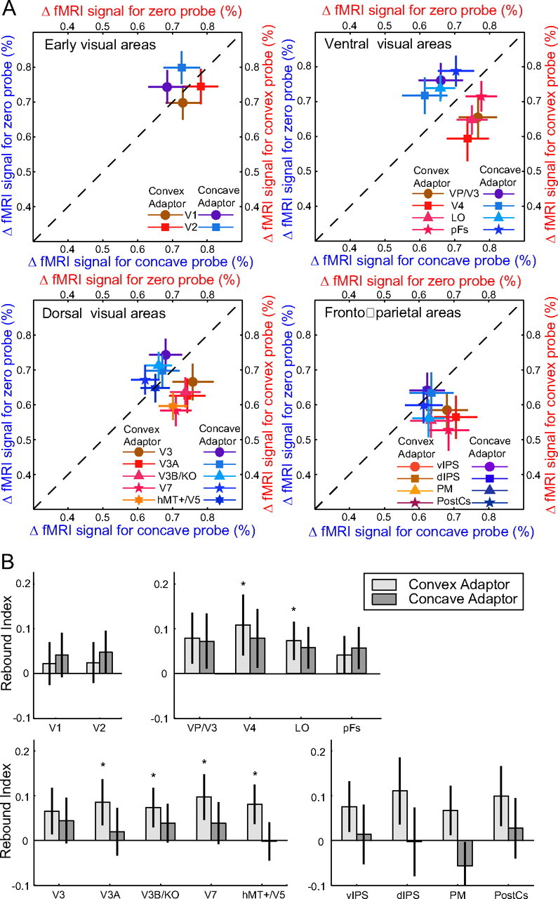
fMRI adaptation for the zero disparity Mach card probe stimulus. A, fMRI responses (percentage signal change from fixation baseline) for the zero probe stimulus are plotted against responses to the corresponding concave and convex probe stimuli across cortical regions of interest. Data for the concave (blue) adaptor show the fMRI response for the zero probe stimulus plotted against the response for the concave probe stimulus (blue axis labels). Data for the convex adaptor (red) show the fMRI response for the zero probe stimulus plotted against the response for the convex probe stimulus (red axis labels). All data were normalized for each area by subtracting the mean response to the adaptor and adding the grand mean across all four adaptor-probe pairs. Error bars are bootstrapped 68% confidence intervals. Displacement from the diagonal dashed line indicates recovery from adaptation. B, Rebound indices for the zero probe stimulus when preceded by the convex or concave adaptor. Error bars show 68% confidence intervals.
Additionally, we tested fMRI selective adaptation for disparity-defined probe stimuli (Fig. 4; supplemental Fig. S3, available at www.jneurosci.org as supplemental material) by comparing fMRI responses evoked by (disparity-defined) convex and concave probes when they were preceded by a (disparity-defined) convex or concave adaptor. We tested for fMRI selective adaptation (i.e., stronger fMRI responses) when the adaptor and probe stimuli differed in their 3D shape (i.e., adaptor-probe pairings: convex–concave, concave–convex) compared with the (adapted) fMRI response evoked when the adaptor and probe stimuli had the same 3D shape (i.e., convex–convex, concave–concave). We found significant fMRI selective adaptation in ventral and dorsal (including the ventral IPS) areas (supplemental Table S3, available at www.jneurosci.org as supplemental material). Figure 4A contrasts the fMRI responses evoked by the convex and concave probe stimuli when they were preceded by a convex or concave adaptor. For the majority of localized regions the data are displaced from the diagonal, indicating recovery from adaptation when adaptor and probe stimuli differed in 3D shape. Quantifying the strength of the recovery using a rebound index (Fig. 4B) showed similar magnitude of fMRI selective adaptation for convex and concave adaptors in both ventral and dorsal cortical areas. This finding suggests that both ventral and dorsal cortical areas are sensitive to differences in disparity-defined shape independent of the shape of the adaptor.
Figure 4.
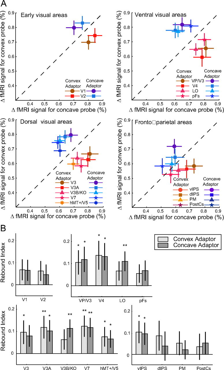
fMRI selective adaptation for concave and convex probe stimuli. A, fMRI responses (percentage signal change from fixation baseline) for the convex probe stimulus plotted against responses to the concave probe stimulus across cortical regions of interest. Data for the convex (red) and concave (blue) adaptor were normalized for each area by subtracting the mean response to the adaptor and adding the grand mean across all four adaptor-probe pairs. Time course and raw fMRI data are shown in supplemental Figure S3, available at www.jneurosci.org as supplemental material. Error bars are bootstrapped 68% confidence intervals. Displacement from the diagonal dashed line indicates recovery from adaptation. B, Rebound indices for the convex and concave probe stimuli across areas. This index indicates the difference in the fMRI responses for trials where adaptor and probe stimulus matched and trials where adaptor and probe stimulus differed. A positive index indicates recovery from adaptation (rebound effect). Error bars are bootstrapped 68% confidence intervals.
However, comparing fMRI-selective adaptation effects for the zero disparity probe (Fig. 3B) and the disparity-defined probe stimuli (Fig. 4B) suggest differential role of ventral and dorsal areas in 3D shape estimation. In particular, the asymmetry observed in the rebound effects between convex and concave adaptors was specific to the ambiguous probe stimulus and was not observed for the disparity-defined probe stimuli (F(14,70) = 0.63, p = 0.83), in line with the perceptual effects we measured. This was confirmed by a significant interaction (F(14,70) = 2.31, p = 0.011) between the adaptor (convex, concave) and the probe stimulus type (zero, disparity-defined).
Together, these findings suggest cortical representations for 3D stimuli that vary in accordance with the observers' perceptual interpretation. Specifically, fMRI rebound effects in dorsal cortical areas and fronto-parietal regions reflect sensitivity to the perceived 3D structure of ambiguous figures as shaped by adaptation. In contrast, rebound effects in ventral areas (V4, LO) reflect sensitivity to changes in depth structure but show weaker modulation in line with the behavioral aftereffect.
fMRI selective adaptation for ambiguous kinetic depth stimuli
The fMRI adaptation asymmetry we observed for the Mach card stimulus is consistent with the pattern of behavioral aftereffects, suggesting a link between cortical responses and the perception of 3D shape. Several control analyses (detailed below) suggested that this was unlikely to result from differential responses to the disparity information in the stimuli within the main dorsal areas of interest. However, to provide a stronger test of these findings, and establish their generality, we chose to study depth aftereffects in bistable 3D stimuli in which disparity information was not informative. We used half cylinders (Fig. 1C) whose 3D structure can be perceived based on the movement of surface markers as the cylinder rotates around its vertical axis (KDE). Without additional information, the stimulus is ambiguous, and observers alternate between convex and concave interpretations, although they show a strong bias for convex interpretations (81% of trials). Adding texture and shading cues disambiguated the stimulus, allowing us to study the effect of adaptation to this stimulus on the perception and cortical representation of the bistable stimulus.
In line with the results from the Mach card, we observed a behavioral repulsion aftereffect (Fig. 1F) for the ambiguous KDE stimulus when it was preceded by a texture- and shading-defined adaptor (Nawrot and Blake, 1989). This change in perceived 3D shape relative to baseline was larger for the convex than the concave adapting stimulus (t2 = 21.4, p = 0.002) similar to the asymmetry observed for the Mach card stimulus (Fig. 1E). Consistent with this asymmetry, we observed significantly (F(1,2) = 52.50, p = 0.02) stronger fMRI rebound effects for convex than concave stimuli (Fig. 5A). Moreover, contrasting the response asymmetry between dorsal and ventral regions for the KDE data, confirmed stronger asymmetries in dorsal areas (t2 = 5.972, p = 0.027). Comparing the asymmetries in the fMRI response for the ambiguous Mach card and the ambiguous KDE stimuli (Fig. 5B), confirmed differences of asymmetry (i.e., higher fMRI selective adaptation for convex than concave adapting stimuli) across visual areas (F(12,96) = 2.389, p = 0.010 main effect of ROI) for both types of ambiguous stimuli and adaptors disambiguated by different cues. To determine the regions in which this asymmetry was statistically reliable, we performed t tests on the mean asymmetry across ROIs within each region against zero (no asymmetry). This revealed significant asymmetry effects (differences between convex and concave adaptor effects) in dorsal (t8 = 4.920, p = 0.001) and parietal areas (t8 = 4.648, p = 0.002) but not in ventral (t8 = 1.636, p = 0.141) or early visual areas (t8 = 0.006, p = 0.995). Previous imaging studies have implicated both ventral and dorsal regions in the processing of 3D shape from monocular cues (Orban et al., 1999; Sereno et al., 2002; Vanduffel et al., 2002; Murray et al., 2003; Peuskens et al., 2004; Georgieva et al., 2008). The similar behavioral repulsion and fMRI rebound effects observed in our study for different ambiguous 3D stimuli suggest common neural substrates mainly in dorsal visual areas for depth aftereffects independent of the cues (disparity, texture, shading) used to define the adapting stimulus.
Figure 5.
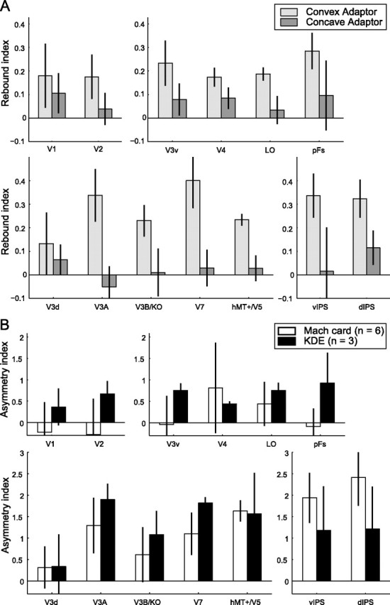
fMRI adaptation for the ambiguous KDE probe stimulus. A, Rebound indices for the ambiguous KDE stimulus when preceded by a concave or convex adapting stimulus. Error bars show 68% confidence intervals. B, A comparison between the asymmetry in the rebound indices for the ambiguous Mach card and KDE stimuli. Data are expressed as asymmetry index that contrasts the fMRI rebound effect for the ambiguous probe stimulus following a period of adaptation to convex and concave stimuli. The index is normalized between experiments (rebound effects were stronger for the denser KDE stimulus) by equating the mean rebound effect across all conditions and ROIs. This normalization of the rebound data can result in an asymmetry index above one. Error bars indicate SEM.
To test the link between behavioral performance and fMRI responses further, we compared individual differences in the asymmetry of the behavioral and fMRI effects. In particular, we conducted a linear regression of fMRI asymmetry on behavioral asymmetry using the individual subjects data (nine in total). This provided evidence for significant relationships between fMRI and behavioral asymmetry in areas V3A (r = 0.815, p = 0.007) and V7 (r = 0.756, p = 0.018) (supplemental Table S4, available at www.jneurosci.org as supplemental material), consistent with the higher fMRI asymmetry observed in dorsal rather than ventral areas.
Control experiments
Our analyses relating fMRI rebound and behavioral repulsion effects point to cortical representations that vary in a perceptually relevant manner. Nevertheless, we controlled for the alternative possibility that differential responses to the stimuli themselves may be responsible for the higher rebound effect for the convex than concave adaptor. Specifically, we found no significant differences between fMRI responses to convex and concave Mach card stimuli when they followed a period of adaptation to a flat, non-3D adapting stimulus (supplemental Fig. S4, supplemental Table S3, available at www.jneurosci.org as supplemental material). We also tested the possibility that weaker responses to far (uncrossed) disparities than near (crossed) disparities may result in weaker rebound effects for the concave adaptor. We measured fMRI responses when concave and convex Mach cards were presented at different depth positions (at, in front, and behind the fixation point). Consistent with a population preference for near disparities (Prince et al., 2002; DeAngelis and Uka, 2003; Preston et al., 2008), we observed significant linear regressions of fMRI response on stimulus disparity in retinotopic visual areas (V1, V2, V3, V3A) and hMT+/V5 (supplemental Fig. S5A, supplemental Table S5, available at www.jneurosci.org as supplemental material) reflecting higher responses for near disparities. Importantly, no significant relationships were observed for higher ventral (V4, LO), dorsal (V3B/KO, V7) and fronto-parietal regions. This suggests that rebound effects in these areas cannot be explained solely by the disparity content of the stimuli, a result bolstered by our findings with the KDE stimulus in which disparity signals were not informative. In addition, low-level cues are unlikely to account for fMRI rebound effects for the KDE stimuli, as luminance and texture size were matched between the adaptor and probe stimuli. Thus, fMRI rebound effects observed in V3A and hMT+/V5 for the KDE stimulus could not be due to low-level monocular cues. However, as fMRI rebound effects in these areas could relate to stimulus disparity content (supplemental Fig. S5A, supplemental Table S5, available at www.jneurosci.org as supplemental material), the relation between fMRI adaptation effects and the perceived 3D shape independent of the adapting cues appears weaker in V3A and hMT+/V5. Together, results from the Mach card, KDE and control experiments suggest that responses in dorsal cortical areas reflect the representation of perceived 3D shape rather than low-level image features.
The relationship between fMRI and behavioral effects could not be explained on the basis of differences in the attentional state or the task difficulty. In line with previous studies (Huk et al., 2001), observers performed a dual task that ensured that they attended similarly across conditions and neither performance nor reaction times differed between conditions (supplemental Fig. S1E, available at www.jneurosci.org as supplemental material). Finally, measures of eye movements suggested that observers were able to maintain fixation well and that there were no systematic differences between conditions (supplemental Fig. S6, available at www.jneurosci.org as supplemental material). Furthermore, we took a number of precautions to ensure that eye vergence changes did not contribute to differences between conditions. First, nonius lines were provided to promote appropriate eye vergence. Second, as part of the control experiment in which stimuli were presented with different disparities, observers performed a subjective assessment of eye vergence (Popple et al., 1998) that suggested vergence was stable despite disparity manipulations (supplemental Fig. S6C, available at www.jneurosci.org as supplemental material). Third, no significant differences (F(1,4) = 0.785, p = 0.43) were observed between fMRI responses when observers made eye movements to points in front or behind the fixation plane with disparities chosen from the Mach card stimuli (supplemental Fig. S5B, available at www.jneurosci.org as supplemental material). Thus, it is unlikely that eye vergence significantly confounded fMRI responses to the stimuli in the regions of interest examined in our study.
Discussion
Estimating the 3D structure of the environment is a principle goal of the visual system. The brain exploits a range of different sensory cues for the purpose as well as incorporating information gained through previous experience to resolve the inherent ambiguities (Sinha and Poggio, 1996; Bülthoff et al., 1998). Here, we examine depth aftereffects to investigate the cortical circuits that mediate the perceptual estimation of 3D structure from ambiguous sensory signals. Although previous imaging studies have used fMRI adaptation to study aftereffects related to the perception of basic visual features (e.g., motion) (Tootell et al., 1995b; He et al., 1998; Culham et al., 1999; Huk et al., 2001) to our knowledge, no previous physiological or fMRI studies have investigated the perceptual aftereffects following adaptation to 3D shape. Using two different ambiguous depth figures, we demonstrate that fMRI adaptation responses in dorsal cortical areas (V3B/KO, V7 and IPS) are consistent with the perceptual 3D aftereffect. These findings suggest that depth processing in these areas relates to the interpretation of ambiguous depth signals as guided by the adaptive context.
We first identified a large network of areas that showed activity associated with spontaneous changes in the perceptual interpretation of constant, ambiguous visual input. This network included ventral (VP/V3, V4, LO), dorsal (V3A, V3B/KO, V7), parietal [vIPS, dorsal intraparietal sulcus (dIPS)] and frontal (PM, PostCS) regions. We then showed that adapting to a relatively unambiguous stimulus (disparity-defined Mach card or texture and shading defined KDE stimulus) had a strong influence on the perceptual interpretation and cortical representation of a subsequently presented ambiguous stimulus in dorsal cortical regions with weaker effects in ventral areas. In contrast, similar adaptation effects were observed in both ventral and dorsal areas (Fig. 4; supplemental Fig. S3, available at www.jneurosci.org as supplemental material) when adaptation and probe stimuli were defined by binocular or monocular depth cues. These results suggest that the asymmetry in fMRI adaptation (i.e., stronger fMRI rebound for convex that concave stimuli) observed in dorsal cortical areas could not be simply due to differential adaptive properties of neural populations in these areas but rather reflects neural processes consistent with the perceptual aftereffect. Our control experiments ruled out explanations based on low-level stimulus properties or artifacts related to eye movements or attention.
Previous studies using electrophysiology and brain imaging (for review, see Orban et al., 2006; Parker, 2007) have implicated both ventral and dorsal cortical areas in processing depth information. Our results suggest that there is a differential recruitment of cortical areas engaged in 3D shape estimation in different contexts. In cases of relatively unambiguous sensory input, sensory evidence about depth structure is processed in a network of ventral and dorsal visual areas. However, when the depth structure is more ambiguous, fMRI responses related to the perceptual aftereffect are manifest in higher dorsal areas and fronto-parietal regions rather than ventral areas. Although inferring interactions between these networks from fMRI data is difficult, it is possible that fronto-parietal regions guide the selection of competing perceptual interpretations and may modulate the processing of depth structure in dorsal cortical areas. Intriguingly, the commonalities between these two networks are centered on the junction between dorsal visual cortex and posterior parietal cortex (V3B/KO, V7, IPS), suggesting a confined ensemble of areas intricately involved in the estimation of 3D shape structure based on different depth cues.
Adaptation to depth structure
At what level does the adaptive processing related to depth aftereffects occur? Psychophysical evidence suggests that while adaptation to fronto-parallel planes may be mediated by the low-level disparity content (Kohler and Emery, 1947; Blakemore and Julesz, 1971; Long and Over, 1973), adaptation to slanted and curved surfaces (as we have used here) occurs at a level beyond the computation of local disparities (Domini et al., 2001; Berends et al., 2005; Knapen and van Ee, 2006). In line with these behavioral studies, the lack of significant adaptation in early visual areas (V1, V2) suggests the processing of depth structure rather than low-level feature analysis. The fMRI rebound effects we observed in ventral and dorsal cortical areas for disparity-defined Mach card stimuli indicate neural populations sensitive to disparity-defined depth. This is consistent with electrophysiology (Janssen et al., 2000; Taira et al., 2000; Uka and DeAngelis, 2004; Tanabe et al., 2005) and imaging studies (Backus et al., 2001; Tsao et al., 2003; Neri et al., 2004; Tyler et al., 2006; Chandrasekaran et al., 2007; Preston et al., 2008; Georgieva et al., 2009). However, the correspondence between fMRI rebound and behavioral repulsion effects for the ambiguous (zero disparity) probe stimulus in dorsal cortical areas (V3B/KO, V7, IPS) suggests neural representations related to perceived 3D shape rather than simply disparity. Moreover, our replication of the main results using the KDE stimulus strengthens this conclusion in suggesting adaptive estimation of 3D structure using information from both binocular and monocular depth cues.
One means of conceptualizing adaptive effects is that they correspond to fatigue in a subset of neurons tuned to different stimulus types (e.g., a habituated response to convex shapes). Such fatigue models have been proposed in relation to the population readout of signals (Barlow and Hill, 1963) where fatigue is believed to cause an imbalance between competing perceptual alternatives. An alternative interpretation is that, as an adaptive system, the brain strives to optimize its response to sensory input based on the prevailing statistics of the environment (Barlow, 1990; Wainwright, 1999; Clifford et al., 2007). Thus, adaptation can be viewed as increasing the resources available to encode differences from the adapting stimulus (Stocker and Simoncelli, 2005). In our case, the task of the visual system is to select the most likely interpretation of the ambiguous depth stimuli, a process often characterized as extracting the peak of a probability distribution representing the continuum of possible shapes (Knill et al., 1996; Mamassian et al., 2002). For the bistable stimuli we employ, this distribution is likely to be bimodal (i.e., one convex peak, one concave peak), with competition between these two modes responsible for the alternating perceptual interpretations. Through adaptation, we expect enhanced sensory encoding around the adapting stimulus (Stocker and Simoncelli, 2005) but an overall lowering of the mode of the likelihood associated with the adapting stimulus. As a result the perceptual interpretation is biased away from the adapting stimulus (i.e., a repulsion aftereffect). Such a change in sensory encoding provides a means of internalizing information about the environment at shorter timescales than the longer-term process of acquiring previous knowledge important in depth perception (Sinha and Poggio, 1996; Bülthoff et al., 1998; Mamassian and Goutcher, 2001).
The short-term repulsive aftereffects we measured contrast with the role of longer term priors that increase the probability of perceiving a stimulus in a given configuration (for instance, a bias for convexity). A number of recent psychophysical studies have considered priming or sensitization due to brief exposure (Kanai and Verstraten, 2005; Maloney et al., 2005; Klink et al., 2008) that results in attractive (rather than repulsive) effects when viewing ambiguous figures. In particular, presenting the same ambiguous figure intermittently will stabilize the observer's interpretation of the stimulus for a prolonged period (Leopold et al., 2002; Fang and He, 2004) and presenting a very brief stimulus can prime the interpretation of a subsequently viewed stimulus (Kanai and Verstraten, 2005; Klink et al., 2008). Similar effects have been observed with fMRI, suggesting priming related effects caused by the recent stimulus presentations (Moore and Engel, 2001). Adapted fMRI responses observed when repeating a stimulus have been attributed to reduction in the gain of the underlying neural response and/or retuning of the neural response (Grill-Spector et al., 2006; Krekelberg et al., 2006; Schlack et al., 2007). The 4 s adaptation period used in our study (Fang et al., 2005), and the repulsive aftereffects we observe (Klink et al., 2008), are most consistent with a gain change interpretation of fMRI adaptation. Finally, it is important to note that our fMRI findings relate to adaptive neural processing at the scale of large neural populations as measured by fMRI rather than selectivity at the level of single neurons. Further combined imaging and physiological studies are necessary to discern the relationship between behavioral repulsion, fMRI adaptation and neuronal selectivity in the areas we have investigated (Grill-Spector et al., 2006; Krekelberg et al., 2006; Sawamura et al., 2006).
In summary, here we study depth aftereffects using bistable stimuli to gain insight into the neural basis of 3D shape perception when the sensory input remains ambiguous but the perceptual interpretation is guided by adaptation. Our findings suggest an important role of dorsal cortical areas (V3B/KO, V7 and IPS) in 3D shape estimation, representing the depth structure of ambiguous signals in line with aftereffects produced by binocular or monocular depth cues. These adaptive effects rely on rapid changes in the brain's use of sensory signals that persist for a short time. Whether the same cortical circuits are involved in combining sensory input with long-term internalized statistical regularities (Knill et al., 1996; Mamassian et al., 2002), learning (Sinha and Poggio, 1996; Bülthoff et al., 1998) and sensory recalibration (Adams et al., 2004) remains an open and intriguing question for future investigation.
Footnotes
This work was supported by the Biotechnology and Biological Sciences Research Council (Grants C520620 and D52199X). We thank V. Conrad for help with pilot work and M. Dexter for technical support. We also thank C. Clifford, R. van Ee, E. Graf, D. Leopold, P. Mamassian, and R. van Wezel for comments and suggestions on this manuscript.
References
- Adams WJ, Graf EW, Ernst MO. Experience can change the ‘light-from-above’ prior. Nat Neurosci. 2004;7:1057–1058. doi: 10.1038/nn1312. [DOI] [PubMed] [Google Scholar]
- Andrews TJ, Schluppeck D, Homfray D, Matthews P, Blakemore C. Activity in the fusiform gyrus predicts conscious perception of Rubin's vase-face illusion. Neuroimage. 2002;17:890–901. [PubMed] [Google Scholar]
- Backus BT, Fleet DJ, Parker AJ, Heeger DJ. Human cortical activity correlates with stereoscopic depth perception. J Neurophysiol. 2001;86:2054–2068. doi: 10.1152/jn.2001.86.4.2054. [DOI] [PubMed] [Google Scholar]
- Barlow HB. A theory about the functional role and synaptic mechanism of visual after-effects. In: Blakemore C, Adler K, Pointon M, editors. Vision: coding and efficiency. Cambridge: Cambridge UP; 1990. pp. 363–375. [Google Scholar]
- Barlow HB, Hill RM. Evidence for a physiological explanation of the waterfall phenomenon and figural after-effects. Nature. 1963;200:1345–1347. doi: 10.1038/2001345a0. [DOI] [PubMed] [Google Scholar]
- Berends EM, Liu B, Schor CM. Stereo-slant adaptation is high level and does not involve disparity coding. J Vis. 2005;5:71–80. doi: 10.1167/5.1.7. [DOI] [PubMed] [Google Scholar]
- Bergman R, Gibson JJ. The negative aftereffect of the perception of a surface slanted in the 3rd dimension. Am J Psychol. 1959;72:364–374. [Google Scholar]
- Blakemore C, Julesz B. Stereoscopic depth aftereffect produced without monocular cues. Science. 1971;171:286–288. doi: 10.1126/science.171.3968.286. [DOI] [PubMed] [Google Scholar]
- Boynton GM, Finney EM. Orientation-specific adaptation in human visual cortex. J Neurosci. 2003;23:8781–8787. doi: 10.1523/JNEUROSCI.23-25-08781.2003. [DOI] [PMC free article] [PubMed] [Google Scholar]
- Brouwer GJ, van Ee R, Schwarzbach J. Activation in visual cortex correlates with the awareness of stereoscopic depth. J Neurosci. 2005;25:10403–10413. doi: 10.1523/JNEUROSCI.2408-05.2005. [DOI] [PMC free article] [PubMed] [Google Scholar]
- Bülthoff I, Bülthoff H, Sinha P. Top-down influences on stereoscopic depth-perception. Nat Neurosci. 1998;1:254–257. doi: 10.1038/699. [DOI] [PubMed] [Google Scholar]
- Chandrasekaran C, Canon V, Dahmen JC, Kourtzi Z, Welchman AE. Neural correlates of disparity-defined shape discrimination in the human brain. J Neurophysiol. 2007;97:1553–1565. doi: 10.1152/jn.01074.2006. [DOI] [PubMed] [Google Scholar]
- Clifford CW, Webster MA, Stanley GB, Stocker AA, Kohn A, Sharpee TO, Schwartz O. Visual adaptation: neural, psychological and computational aspects. Vision Res. 2007;47:3125–3131. doi: 10.1016/j.visres.2007.08.023. [DOI] [PubMed] [Google Scholar]
- Culham JC, Dukelow SP, Vilis T, Hassard FA, Gati JS, Menon RS, Goodale MA. Recovery of fMRI activation in motion area MT following storage of the motion aftereffect. J Neurophysiol. 1999;81:388–393. doi: 10.1152/jn.1999.81.1.388. [DOI] [PubMed] [Google Scholar]
- DeAngelis GC, Uka T. Coding of horizontal disparity and velocity by MT neurons in the alert macaque. J Neurophysiol. 2003;89:1094–1111. doi: 10.1152/jn.00717.2002. [DOI] [PubMed] [Google Scholar]
- DeYoe EA, Carman GJ, Bandettini P, Glickman S, Wieser J, Cox R, Miller D, Neitz J. Mapping striate and extrastriate visual areas in human cerebral cortex. Proc Natl Acad Sci U S A. 1996;93:2382–2386. doi: 10.1073/pnas.93.6.2382. [DOI] [PMC free article] [PubMed] [Google Scholar]
- Domini F, Adams W, Banks MS. 3D after-effects are due to shape and not disparity adaptation. Vision Res. 2001;41:2733–2739. doi: 10.1016/s0042-6989(01)00161-4. [DOI] [PubMed] [Google Scholar]
- Dupont P, De Bruyn B, Vandenberghe R, Rosier AM, Michiels J, Marchal G, Mortelmans L, Orban GA. The kinetic occipital region in human visual cortex. Cereb Cortex. 1997;7:283–292. doi: 10.1093/cercor/7.3.283. [DOI] [PubMed] [Google Scholar]
- Efron B, Tibshirani RJ. An introduction to the bootstrap. Boca Raton, FL: Chapman and Hall/CRC; 1993. [Google Scholar]
- Engel SA, Rumelhart DE, Wandell BA, Lee AT, Glover GH, Chichilnisky EJ, Shadlen MN. fMRI of human visual cortex. Nature. 1994;369:525. doi: 10.1038/369525a0. [DOI] [PubMed] [Google Scholar]
- Fang F, He S. Stabilized structure from motion without disparity induces disparity adaptation. Curr Biol. 2004;14:247–251. doi: 10.1016/j.cub.2004.01.031. [DOI] [PubMed] [Google Scholar]
- Fang F, Murray SO, Kersten D, He S. Orientation-tuned FMRI adaptation in human visual cortex. J Neurophysiol. 2005;94:4188–4195. doi: 10.1152/jn.00378.2005. [DOI] [PubMed] [Google Scholar]
- Georgieva S, Peeters R, Kolster H, Todd JT, Orban GA. The processing of 3D shape from disparity in the human brain. J Neurosci. 2009;29:727–742. doi: 10.1523/JNEUROSCI.4753-08.2009. [DOI] [PMC free article] [PubMed] [Google Scholar]
- Georgieva SS, Todd JT, Peeters R, Orban GA. The extraction of 3D shape from texture and shading in the human brain. Cereb Cortex. 2008;18:2416–2438. doi: 10.1093/cercor/bhn002. [DOI] [PMC free article] [PubMed] [Google Scholar]
- Grill-Spector K, Henson R, Martin A. Repetition and the brain: neural models of stimulus-specific effects. Trends Cogn Sci. 2006;10:14–23. doi: 10.1016/j.tics.2005.11.006. [DOI] [PubMed] [Google Scholar]
- He S, Cohen ER, Hu X. Close correlation between activity in brain area MT/V5 and the perception of a visual motion aftereffect. Curr Biol. 1998;8:1215–1218. doi: 10.1016/s0960-9822(07)00512-x. [DOI] [PubMed] [Google Scholar]
- Huk AC, Ress D, Heeger DJ. Neuronal basis of the motion aftereffect reconsidered. Neuron. 2001;32:161–172. doi: 10.1016/s0896-6273(01)00452-4. [DOI] [PubMed] [Google Scholar]
- Janssen P, Vogels R, Orban GA. Selectivity for 3D shape that reveals distinct areas within macaque inferior temporal cortex. Science. 2000;288:2054–2056. doi: 10.1126/science.288.5473.2054. [DOI] [PubMed] [Google Scholar]
- Kanai R, Verstraten FA. Perceptual manifestations of fast neural plasticity: motion priming, rapid motion aftereffect and perceptual sensitization. Vision Res. 2005;45:3109–3116. doi: 10.1016/j.visres.2005.05.014. [DOI] [PubMed] [Google Scholar]
- Kleinschmidt A, Büchel C, Zeki S, Frackowiak RS. Human brain activity during spontaneously reversing perception of ambiguous figures. Proc Biol Sci. 1998;265:2427–2433. doi: 10.1098/rspb.1998.0594. [DOI] [PMC free article] [PubMed] [Google Scholar]
- Klink PC, van Ee R, Nijs MM, Brouwer GJ, Noest AJ, van Wezel RJA. Early interactions between neuronal adaptation and voluntary control determine perceptual choices in bistable vision. J Vis. 2008;8:1–18. doi: 10.1167/8.5.16. [DOI] [PubMed] [Google Scholar]
- Knapen T, van Ee R. Slant perception, and its voluntary control, do not govern the slant aftereffect: multiple slant signals adapt independently. Vision Res. 2006;46:3381–3392. doi: 10.1016/j.visres.2006.03.027. [DOI] [PubMed] [Google Scholar]
- Knill DC, Kersten D, Yuille A. A Bayesian formulation of visual perception. In: Knill DC, Richards W, editors. Perception as Bayesian inference. Cambridge: Cambridge UP; 1996. pp. 1–22. [Google Scholar]
- Kohler W, Emery DA. Figural after-effects in the 3rd dimension of visual space. Am J Psychology. 1947;60:159–201. [PubMed] [Google Scholar]
- Kourtzi Z, Kanwisher N. Cortical regions involved in perceiving object shape. J Neurosci. 2000;20:3310–3318. doi: 10.1523/JNEUROSCI.20-09-03310.2000. [DOI] [PMC free article] [PubMed] [Google Scholar]
- Krekelberg B, Boynton GM, van Wezel RJ. Adaptation: from single cells to BOLD signals. Trends Neurosci. 2006;29:250–256. doi: 10.1016/j.tins.2006.02.008. [DOI] [PubMed] [Google Scholar]
- Langer MS, Bülthoff HH. A prior for global convexity in local shape-from-shading. Perception. 2001;30:403–410. doi: 10.1068/p3178. [DOI] [PubMed] [Google Scholar]
- Leopold DA, Wilke M, Maier A, Logothetis NK. Stable perception of visually ambiguous patterns. Nat Neurosci. 2002;5:605–609. doi: 10.1038/nn0602-851. [DOI] [PubMed] [Google Scholar]
- Liu B, Todd JT. Perceptual biases in the interpretation of 3D shape from shading. Vision Res. 2004;44:2135–2145. doi: 10.1016/j.visres.2004.03.024. [DOI] [PubMed] [Google Scholar]
- Long N, Over R. Stereoscopic depth aftereffects with random-dot patterns. Vision Res. 1973;13:1283–1287. doi: 10.1016/0042-6989(73)90203-4. [DOI] [PubMed] [Google Scholar]
- Lumer ED, Friston KJ, Rees G. Neural correlates of perceptual rivalry in the human brain. Science. 1998;280:1930–1934. doi: 10.1126/science.280.5371.1930. [DOI] [PubMed] [Google Scholar]
- Mach E. The analysis of sensations. New York: Dover; 1886. [Google Scholar]
- Maloney LT, Dal Martello MF, Sahm C, Spillmann L. Past trials influence perception of ambiguous motion quartets through pattern completion. Proc Natl Acad Sci U S A. 2005;102:3164–3169. doi: 10.1073/pnas.0407157102. [DOI] [PMC free article] [PubMed] [Google Scholar]
- Mamassian P, Goutcher R. Prior knowledge on the illumination position. Cognition. 2001;81:B1–B9. doi: 10.1016/s0010-0277(01)00116-0. [DOI] [PubMed] [Google Scholar]
- Mamassian P, Landy M, Maloney L. Bayesian modelling of visual perception. In: Rao RPN, Olshausen BA, Lewicki MS, editors. Probabilistic models of the brain. Cambridge, MA: MIT; 2002. pp. 13–36. [Google Scholar]
- Moore C, Engel SA. Neural response to perception of volume in the lateral occipital complex. Neuron. 2001;29:277–286. doi: 10.1016/s0896-6273(01)00197-0. [DOI] [PubMed] [Google Scholar]
- Murray SO, Olshausen BA, Woods DL. Processing shape, motion and three-dimensional shape-from-motion in the human cortex. Cereb Cortex. 2003;13:508–516. doi: 10.1093/cercor/13.5.508. [DOI] [PubMed] [Google Scholar]
- Nawrot M, Blake R. Neural integration of information specifying structure from stereopsis and motion. Science. 1989;244:716–718. doi: 10.1126/science.2717948. [DOI] [PubMed] [Google Scholar]
- Nawrot M, Blake R. The interplay between stereopsis and structure from motion. Percept Psychophys. 1991;49:230–244. doi: 10.3758/bf03214308. [DOI] [PubMed] [Google Scholar]
- Neri P, Bridge H, Heeger DJ. Stereoscopic processing of absolute and relative disparity in human visual cortex. J Neurophysiol. 2004;92:1880–1891. doi: 10.1152/jn.01042.2003. [DOI] [PubMed] [Google Scholar]
- Orban GA, Sunaert S, Todd JT, Van Hecke P, Marchal G. Human cortical regions involved in extracting depth from motion. Neuron. 1999;24:929–940. doi: 10.1016/s0896-6273(00)81040-5. [DOI] [PubMed] [Google Scholar]
- Orban GA, Janssen P, Vogels R. Extracting 3D structure from disparity. Trends Neurosci. 2006;29:466–473. doi: 10.1016/j.tins.2006.06.012. [DOI] [PubMed] [Google Scholar]
- Parker AJ. Binocular depth perception and the cerebral cortex. Nat Rev Neurosci. 2007;8:379–391. doi: 10.1038/nrn2131. [DOI] [PubMed] [Google Scholar]
- Peuskens H, Claeys KG, Todd JT, Norman JF, Van Hecke P, Orban GA. Attention to 3-D shape, 3-D motion, and texture in 3-D structure from motion displays. J Cogn Neurosci. 2004;16:665–682. doi: 10.1162/089892904323057371. [DOI] [PubMed] [Google Scholar]
- Polonsky A, Blake R, Braun J, Heeger DJ. Neuronal activity in human primary visual cortex correlates with perception during binocular rivalry. Nat Neurosci. 2000;3:1153–1159. doi: 10.1038/80676. [DOI] [PubMed] [Google Scholar]
- Popple AV, Smallman HS, Findlay JM. The area of spatial integration for initial horizontal disparity vengeance. Vision Res. 1998;38:319–326. doi: 10.1016/s0042-6989(97)00166-1. [DOI] [PubMed] [Google Scholar]
- Press WA, Brewer AA, Dougherty RF, Wade AR, Wandell BA. Visual areas and spatial summation in human visual cortex. Vision Res. 2001;41:1321–1332. doi: 10.1016/s0042-6989(01)00074-8. [DOI] [PubMed] [Google Scholar]
- Preston TJ, Li S, Kourtzi Z, Welchman AE. Multivoxel pattern selectivity for perceptually relevant binocular disparities in the human brain. J Neurosci. 2008;28:11315–11327. doi: 10.1523/JNEUROSCI.2728-08.2008. [DOI] [PMC free article] [PubMed] [Google Scholar]
- Prince SJ, Cumming BG, Parker AJ. Range and mechanism of encoding of horizontal disparity in macaque V1. J Neurophysiol. 2002;87:209–221. doi: 10.1152/jn.00466.2000. [DOI] [PubMed] [Google Scholar]
- Sawamura H, Orban GA, Vogels R. Selectivity of neuronal adaptation does not match response selectivity: a single-cell study of the FMRI adaptation paradigm. Neuron. 2006;49:307–318. doi: 10.1016/j.neuron.2005.11.028. [DOI] [PubMed] [Google Scholar]
- Schlack A, Krekelberg B, Albright TD. Recent history of stimulus speeds affects the speed tuning of neurons in area MT. J Neurosci. 2007;27:11009–11018. doi: 10.1523/JNEUROSCI.3165-07.2007. [DOI] [PMC free article] [PubMed] [Google Scholar]
- Sereno ME, Trinath T, Augath M, Logothetis NK. Three-dimensional shape representation in monkey cortex. Neuron. 2002;33:635–652. doi: 10.1016/s0896-6273(02)00598-6. [DOI] [PubMed] [Google Scholar]
- Sereno MI, Dale AM, Reppas JB, Kwong KK, Belliveau JW, Brady TJ, Rosen BR, Tootell RBH. Borders of multiple visual areas in humans revealed by functional magnetic-resonance-imaging. Science. 1995;268:889–893. doi: 10.1126/science.7754376. [DOI] [PubMed] [Google Scholar]
- Sinha P, Poggio T. Role of learning in three-dimensional form perception. Nature. 1996;384:460–463. doi: 10.1038/384460a0. [DOI] [PubMed] [Google Scholar]
- Stocker AA, Simoncelli EP. Constraining a Bayesian model of human visual speed perception. In: Schölkopf B, Platt J, Weiss Y, editors. Advances in neural information processing systems NIPS. Cambridge, MA: MIT; 2005. pp. 1291–1298. [Google Scholar]
- Taira M, Tsutsui KI, Jiang M, Yara K, Sakata H. Parietal neurons represent surface orientation from the gradient of binocular disparity. J Neurophysiol. 2000;83:3140–3146. doi: 10.1152/jn.2000.83.5.3140. [DOI] [PubMed] [Google Scholar]
- Tanabe S, Doi T, Umeda K, Fujita I. Disparity-tuning characteristics of neuronal responses to dynamic random-dot stereograms in macaque visual area V4. J Neurophysiol. 2005;94:2683–2699. doi: 10.1152/jn.00319.2005. [DOI] [PubMed] [Google Scholar]
- Taya S, Sato M, Nakamizo S. Stereoscopic depth aftereffects without retinal position correspondence between adaptation and test stimuli. Vision Res. 2005;45:1857–1866. doi: 10.1016/j.visres.2005.01.018. [DOI] [PubMed] [Google Scholar]
- Tong F, Meng M, Blake R. Neural bases of binocular rivalry. Trends Cogn Sci. 2006;10:502–511. doi: 10.1016/j.tics.2006.09.003. [DOI] [PubMed] [Google Scholar]
- Tootell RB, Reppas JB, Kwong KK, Malach R, Born RT, Brady TJ, Rosen BR, Belliveau JW. Functional analysis of human MT and related visual cortical areas using magnetic resonance imaging. J Neurosci. 1995a;15:3215–3230. doi: 10.1523/JNEUROSCI.15-04-03215.1995. [DOI] [PMC free article] [PubMed] [Google Scholar]
- Tootell RB, Reppas JB, Dale AM, Look RB, Sereno MI, Malach R, Brady TJ, Rosen BR. Visual motion aftereffect in human cortical area MT revealed by functional magnetic resonance imaging. Nature. 1995b;375:139–141. doi: 10.1038/375139a0. [DOI] [PubMed] [Google Scholar]
- Tootell RB, Hadjikhani N, Hall EK, Marrett S, Vanduffel W, Vaughan JT, Dale AM. The retinotopy of visual spatial attention. Neuron. 1998;21:1409–1422. doi: 10.1016/s0896-6273(00)80659-5. [DOI] [PubMed] [Google Scholar]
- Tsao DY, Vanduffel W, Sasaki Y, Fize D, Knutsen TA, Mandeville JB, Wald LL, Dale AM, Rosen BR, Van Essen DC, Livingstone MS, Orban GA, Tootell RB. Stereopsis activates V3A and caudal intraparietal areas in macaques and humans. Neuron. 2003;39:555–568. doi: 10.1016/s0896-6273(03)00459-8. [DOI] [PubMed] [Google Scholar]
- Tyler CW, Likova LT, Chen CC, Kontsevich LL, Schira MM, Wade AR. Extended concepts of occipital retinotopy. Curr Med Imag Rev. 2005;1:319–329. [Google Scholar]
- Tyler CW, Likova LT, Kontsevich LL, Wade AR. The specificity of cortical region KO to depth structure. Neuroimage. 2006;30:228–238. doi: 10.1016/j.neuroimage.2005.09.067. [DOI] [PubMed] [Google Scholar]
- Uka T, DeAngelis GC. Contribution of area MT to stereoscopic depth perception: Choice-related response modulations reflect task strategy. Neuron. 2004;42:297–310. doi: 10.1016/s0896-6273(04)00186-2. [DOI] [PubMed] [Google Scholar]
- Vanduffel W, Fize D, Peuskens H, Denys K, Sunaert S, Todd JT, Orban GA. Extracting 3D from motion: differences in human and monkey intraparietal cortex. Science. 2002;298:413–415. doi: 10.1126/science.1073574. [DOI] [PubMed] [Google Scholar]
- Wainwright MJ. Visual adaptation as optimal information transmission. Vision Res. 1999;39:3960–3974. doi: 10.1016/s0042-6989(99)00101-7. [DOI] [PubMed] [Google Scholar]
- Wallach H, O'Connell DN. The kinetic depth effect. J Exp Psychol. 1953;45:205–217. doi: 10.1037/h0056880. [DOI] [PubMed] [Google Scholar]
- Zeki S, Watson JD, Lueck CJ, Friston KJ, Kennard C, Frackowiak RS. A direct demonstration of functional specialization in human visual-cortex. J Neurosci. 1991;11:641–649. doi: 10.1523/JNEUROSCI.11-03-00641.1991. [DOI] [PMC free article] [PubMed] [Google Scholar]