Correlating Stimulus-Specific Adaptation of Cortical Neurons and Local Field Potentials in the Awake Rat

Abstract

Changes in the sensory environment are good indicators for behaviorally relevant events and strong triggers for the reallocation of attention. In the auditory domain, violations of a pattern of repetitive stimuli precipitate in the event-related potentials as mismatch negativity (MMN). Stimulus-specific adaptation (SSA) of single neurons in the auditory cortex has been proposed to be the cellular substrate of MMN (Nelken and Ulanovsky, 2007). However, until now, the existence of SSA in the awake auditory cortex has not been shown. In the present study, we recorded single and multiunits in parallel with evoked local field potentials (eLFPs) in the primary auditory cortex of the awake rat. Both neurons and eLFPs in the awake animal adapted in a stimulus-specific manner, and SSA was controlled by stimulus probability and frequency separation. SSA of isolated units was significant during the first stimulus-evoked “on” response but not in the following inhibition and rebound of activity. The eLFPs exhibited SSA in the first negative deflection and, to a lesser degree, in a slower positive deflection but no MMN. Spike adaptation correlated closely with adaptation of the fast negative deflection but not the positive deflection. Therefore, we conclude that single neurons in the auditory cortex of the awake rat adapt in a stimulus-specific manner and contribute to corresponding changes in eLFP but do not generate a late deviant response component directly equivalent to the human MMN. Nevertheless, the described effect may reflect a certain part of the process needed for sound discrimination.

Introduction

The representation of behaviorally relevant stimuli in a noisy and complex environment that consists of multiple signals from different sources is one of the major challenges for the auditory system. The statistics of stimuli provide critical cues for structuring such an environment (Bregman, 1990) for optimizing the neuronal coding of it (Brenner et al., 2000; Kvale and Schreiner, 2004; Dean et al., 2005) and for selecting vital information from it. In this respect, infrequent deviations in a repetitive auditory background are often events of behavioral importance. Such rarely occurring events are represented in the nervous system by a preattentive and automatic auditory process (Näätänen et al., 2007), which is only partially under attentional control (Sussman, 2007).

A correlate in human EEG recordings for neuronal mechanisms of change detection is the so-called mismatch negativity (MMN) that may serve as a trigger for reallocating attention toward the deviants (Escera et al., 1998). Its characteristic feature is a negative wave occurring ∼200 ms after stimulus onset in response to an infrequent deviant stimulus (Dev), which is embedded in a sequence of repetitive standard tones (St). To evoke MMN, the deviant and standard stimuli can be selected from a variety of stimuli (i.e., pure tones, vowels) and differ in various aspects such as frequency (Näätänen et al., 1978), duration (Giard et al., 1995), and level (Schröger, 1996) or even being omitted (Yabe et al., 1997). Different cortical sources contribute to MMN generation with one being the auditory cortex (AC) (Näätänen et al., 2007) or probably only a subdivision of AC (Pincze et al., 2001).

Although there is a large data basis on MMN available, only few publications approach its cellular basis in terms of cortical neuronal response properties. Recently, stimulus-specific adaptation (SSA) has been proposed as a candidate neuronal mechanism underlying the generation of MMN (Ulanovsky et al., 2003; Nelken and Ulanovsky, 2007). In experiments on anesthetized animals, SSA was identified at different stages of the auditory pathway, namely cat AC (Ulanovsky et al., 2003), mouse auditory thalamus (Anderson et al., 2009), and rat inferior colliculus (Malmierca et al., 2009). In addition, there were attempts to demonstrate MMN with means of event-related potentials in rodents (Ruusuvirta et al., 1998; Lazar and Metherate, 2003; Sambeth et al., 2003; Eriksson and Villa, 2005; Umbricht et al., 2005; Astikainen et al., 2006; Tikhonravov et al., 2008), but the resulting patterns are weak or ambiguous.

To address the neuronal basis of MMN, the present study focuses on the awake rat primary auditory cortex (A1). We used both recordings from neurons and evoked local field potentials (eLFPs), which could provide a bridge between cellular properties and EEG recordings. The following questions are addressed. Whether and how is SSA present in neurons of A1 in the awake rat? Do the eLFPs adapt in a similar manner as neurons and do they exhibit an MMN-like pattern? Finally, can we establish a contribution of single neuron adaptation to eLFP adaptation?

Materials and Methods

Subjects and implantation.

Experiments were performed on eight female adult rats weighing 270–370 g at the date of implantation (Sprague Dawley; Charles River Laboratories). All animals were implanted chronically with electrodes in the left auditory cortex under deep anesthesia with chloral hydrate (300 mg · kg⁻¹ · h⁻¹, i.p., Sigma-Aldrich) and ketamine (10 mg · kg⁻¹ · h⁻¹, i.p., Ketavet; Pfizer,) plus atropine (1.2 mg/kg, s.c., administered every 2 h; Sigma-Aldrich). Electrodes were attached to a customized microdrive, carrying three to five tungsten microelectrodes (shaft diameter, 75 μm; impedance before black plating at 1 kHz, 9–12 MΩ; FHC). The drive allowed to move all electrodes simultaneously. Electrodes were oriented in a tangential approach, thereby moving through the auditory cortex in parallel to the cortical layers. Tip-to-tip spacing of electrodes along the rostrocaudal axis was 250–350 μm. A low-impedance silver wire was implanted within the corpus callosum serving as the reference electrode for the extracellular and eLFP recordings. A ground screw was fixed in the temporal bone. The implant was fixed on the skull with dental cement (Haraeus Kulzer). Recordings started at the earliest 10 d after implantation. Animals were trained to sit quietly and with the head oriented forward on an elevated platform in the sound booth within 10 d after implantation. Animals were kept in a light/dark cycle shifted by 12 h. Experimental procedures were in full compliance with federal regulations and to the Guide for the Care and Use of Laboratory Animals (National Research Council, 1996) and approved by the local animal care committee.

Electrophysiological recordings.

All experiments were performed in a sound-attenuating chamber (IAC) during the wake phase of the rats (8:00 A.M. to 8:00 P.M.). Electrodes were advanced before each recording session for between 87 and 175 μm beyond the previous recording site by turning the screws of the implanted microdrive (350 μm per revolution). Each electrode advancement was followed by an interval of at least 15 min to check for clearly separable spikes and let the brain tissue settle. After each recording session, the electrodes were retracted by half of the advanced distance to avoid any disturbance of the next recording location. The recordings were performed in the A1, identified by the tonotopic gradient of characteristic frequencies (CFs) of different units recorded with different electrodes along the rostrocaudal axis and from response properties, such as latency (Rutkowski et al., 2003). In addition, electrode locations were confirmed histologically after recording. An electrolytic lesion marked the start point and endpoint of an electrode track. After transcardially perfusing the animal under deep anesthesia (500 mg of sodium pentobarbital per kilogram of body weight), the brain was sectioned (50 μm thick) and Nissl stained. Electrode tracks were reconstructed from the lesions, and the recording sites were confirmed to be in A1.

The neural signal was preamplified with a custom-made 25-channel head stage (Frank et al., 2001) that was attached to the connector of the microdrive and fixed firmly on the animal's head before every recording session. The signal from each electrode was then separated into a continuously sampled channel for recording LFP signals and a spike channel (extracellular recording). Filtering, amplification, and digitalization of the signals was performed with a Cheetah 32 system (Neuralynx). The LFP signal was filtered at 1–475 Hz, amplified (5000×; Lynx8 Amplifier), and sampled with a rate of 2 kHz, whereas the spike signal was filtered at 600–3000 Hz, amplified with higher gain (20,000×; Lynx8 Amplifier), and inverted. Every spike waveform was sampled with 32 kHz. Cheetah software (Neuralynx) was used for data acquisition. The quality of the spike waveforms and cluster separation from the background was continuously monitored online during the experiments. Additionally, postrecording manual spike sorting was done to select only well isolated units (Spikesort; Neuralynx). Single units (SUs) had <5% of refractory violations (interspike interval <1 ms). After identifying a unit as being stable and well separated, its tuning properties were characterized. In 61 sessions with eight animals, a total of 76 units that fulfilled our selection criteria [27 SUs and 49 multiunits (MUs)] were recorded.

Sound generation.

Acoustic stimuli were presented under free-field conditions. Pure tones were generated with a Tucker-Davis Technologies System 3 with 10 ms rise/fall times. The digital stimuli were converted to the analog signal (RX6), attenuated to the desired level (PA5), and presented by an electrodynamic speaker (ScanSpeak R2904/7000; Tymphany) on the right side of the animal. To achieve a linear speaker output, the systems transfer function was measured with a microphone (model 4939; Brüel & Kjær) and compensated for by filtering the signal with a digital finite impulse response (FIR) filter realized on the signal processor (402 taps, coefficients calculated with function “FIR2,” Matlab 7; MathWorks).

Stimulus design and presentation.

Stimulus presentation and triggering of physiological recording was controlled with a program written in C for experimental control. Frequency response areas were measured using pure tones (100 ms duration) with intensities from −10 or 0 to 60 dB sound pressure level (SPL) and frequencies in the range of 0.5–45 kHz, with logarithmically spaced frequency steps (0.2 or 0.25 octaves). Stimuli were presented in a pseudorandomized sequence at a rate of 1 Hz and with 10–15 repetitions. A tuning curve was calculated immediately afterward, and the CF was determined.

For the adaptation experiment, first a sequence of 800 pure tones (200 ms duration, 1 Hz repetition rate) was presented. In this sequence, a tone could be either a frequently presented standard or a rarely presented deviant differing from the standard in the frequency dimension. In the next sequence, frequencies of standard and deviant were swapped. The complete dataset from both sequences included neural responses to two tones presented each once as standard and once as deviant. The frequencies of the two tones were centered around the CF of a selected unit with frequency 1 (tone f₁) placed below the CF and frequency 2 (tone f₂) placed above the CF (Fig. 1C). In each sequence, the position of the standards and deviants was pseudorandomized, generating sequences with identical deviant probabilities (pDev) but different deviant positions within the sequences. Two stimulus parameters were changed to investigate their influence on adaptation: frequency separation (Δf in octaves) and pDev. Frequency separation was either 0.5 or 0.25 octaves, and deviant probability was either 0.1 or 0.3, adding up to four possible combinations of frequency and probability [condition (pDev/Δf), 01/0.5, 0.1/0.25, 0.3/0.5, and 0.3/0.25]. Additional measurements were done with a deviant probability of 0.5 as control [condition (pDev/Δf), 0.5/0.5]. Another control consisted in the omission of the deviant tone (p = 0.1). All stimuli had a level of 50 dB SPL. Not all of these six stimulus conditions were measured for every unit because unrestrained rats cooperated only a limited time (usually ∼2 h/session and day).

Figure 1.

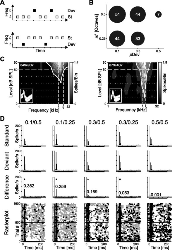
Adaptation paradigm and example data. A, Schema of the stimulation sequence comprising two pure tones of different frequency. After presenting tone f₁ as standard with high probability and tone f₂ as deviant with low probability in pseudorandom order (top sequence), f₂ is presented as standard tone and f₁ as deviant tone in a second sequence (bottom sequence). B, Five stimulus conditions were tested with varying pDev and Δf (in octaves). The number of recorded units for each parameter combination is given and encoded in dot size. The 0.5/0.5 condition is a control. C, Frequency response areas from two example neurons and the respective position of the two tones f₁ and f₂ within the response areas. The left example shows a single unit with f₁ and f₂ separated by ½ octave centered around the units CF. The right example shows a multiunit with two tones separated by ¼ octave. D, Example for an adapting neuron (same unit as in C, left). Depicted are PSTHs for different stimulus conditions [as indicated above the top row (pDev/Δf)]. The rows show neuronal response to f₁ and f₂ together as PSTHs (5 ms bin size) to standard tones, deviant tones, and the difference signal (Dev − St) for five different stimulus conditions. A black bar under PSTHs indicate stimulus duration. Numbers given in the difference PSTH (third row) indicate the sAI for the bin with the highest difference (equivalent to a change of activity of 113.5, 68.9, 40.7, 11.2, and −0.2% from left to right). Bins with a significant difference in activity are indicated in the PSTHs (*p < 0.05). Neuronal responses to all 1600 stimuli are shown as dot plot in the bottom row. Each dot indicates the occurrence of a spike, gray dots for spikes from standard trials, and black dots for spikes from deviant trials.

Data analysis of extracellular recordings.

For every unit, a frequency tuning curve was generated from the frequency response area (Fig. 1C), and the CF was computed. The threshold criterion of the frequency tuning curve was set to 20–40% of the maximum activity measured in the frequency response area. This value had to be adjusted individually in different neurons because of a high background activity in awake animals and the small number of averages. The activity was quantified on the basis of peristimulus time histograms (PSTHs). A linear interpolation algorithm was used for calculating the borders of the tuning curve (function “CONTOURC” in Matlab) and tuning parameters. A 100 ms window preceding the stimuli was used for measuring spontaneous firing rate of each unit. Response latency was determined on the basis of PSTHs as the bin after stimulus onset with maximum activity (in spikes per second, 2 ms bin size). The degree of spike adaptation was quantified using a normalized spike adaptation index (sAI), which is identical to the selectivity index described by Ulanovsky et al. (2003):

where Dev(f₁) and St(f₁) represent spike responses to the tone f₁ as deviant and standard, respectively. The same nomenclature applies for spike responses to tone f₂. Three different time windows were considered for measuring the activity and the adaptation index. Beginning from the stimulus onset, these time windows were 50 and 250 ms long, and one window just comprised the bin with the highest activity for every experimental condition. For analyzing adaptation to the two frequencies separately, the sAI index was calculated for f₁ and f₂ individually.

Data analysis of evoked local field potentials.

Before analyzing the eLFPs, the continuously sampled signal was filtered by applying a fast Fourier transformation (FFT) (function “FFT” in Matlab) to the continuous signal (FFT time window of ∼13 min), removing all frequency components above 50 Hz and below 1 Hz and then recovered with an inverse FFT (function “IFFT” in Matlab). The threshold for artifact rejection was four times the average peak negative amplitude. Two components of the eLFPs were considered for additional analysis: the first fast negative deflection (Nd) and the slower positive deflection (Pd). The latencies of these two components were calculated on the basis of the lowest (for Nd) and highest (for Pd) amplitude of the deflections with a temporal accuracy of 0.5 ms determined by the sampling rate of 2 kHz. Across all sessions, the eLFPs were averaged for each stimulus condition generating a grand mean and an SEM. Adaptation of eLFPs was quantified on the basis of the response amplitude measured as Nd and Pd. Comparable with the spike data, a normalized adaptation index of the eLFP (pAI) was calculated as follows:

where Dev(f_x) and St(f_x) represent the eLFP amplitude in response to deviant tones and standard tones, respectively. The response could be either the negative (Nd) or the positive (Pd) deflection, resulting in two adaptation indices for eLFPs: pAI–Nd and pAI–Pd, respectively.

Correlation analysis of spikes and eLFPs.

For analyzing the relationship between the spike adaptation (sAI) and the adaptation present in the field potential (pAI), the linear correlation between them was computed. For each stimulus configuration, the Spearman's rank correlation coefficient r_s (function “CORR” in Matlab) was computed for sAI versus pAI–Nd and sAI versus pAI–Pd. Significant nonzero correlations are indicated (p < 0.05).

Neuronal receiver operator characteristic.

In analogy to human psychophysical signal detection theory, a neuronal receiver operator characteristic (ROC) was constructed, giving rise to a neurometric detection function for each unit (Barlow et al., 1971). The neuronal ROC was built as described by Stüttgen and Schwarz (2008). The distribution of spike counts was generated for the two stimulus types, deviant and standard. Next, a criterion was shifted through the distributions with a step size of one spike. At each new criterion, the number of spikes above and below it were computed for deviants and the standards. All spike numbers in response to the deviant being above the criterion were considered to be hits, and all spike numbers in response to the standard were considered to be false alarms. For both hits and false alarms, the proportion of the total spike count were computed at each criterion level. By plotting this false alarm rate versus the hit rate, an ROC was generated. The area under the ROC [area under curve (AUC)] is a measure of how well the two distributions of spike numbers (deviant and standard) are separated. To make the AUC values more comparable with the other data, 0.5 was subtracted from it. It then ranges from −0.5 (no overlap in distribution, standard > deviant) to +0.5 (no overlap in distribution, deviant > standard), with 0 corresponding to a total overlap of distributions and thus nonseparability. For the standard ROC analysis, the neuronal response was integrated from 10 to 50 ms after stimulus onset and was pooled for the two stimulation frequencies f₁ and f₂. For analyzing the optimal window duration and position in time allowing the best discrimination between standard and deviant, both were varied in 5 ms steps, with the time windows ranging from 5 to 50 ms duration and the position ranging from 0 to 250 ms after stimulus onset.

Results

We recorded a total of 76 single units and small multiunit clusters (n = 27 and n = 49, respectively) from A1 of the awake rat. For a subset of units, eLFPs were recorded in parallel to the extracellular spike recordings from the same electrode (condition 0.1/0.5: n = 17; condition 0.1/0.25: n = 19; condition 0.3/0.5: n = 10; condition 0.3/0.25: n = 27). The frequency response area was characterized for each unit, and, depending on its CF, two frequencies, symmetrically centered around the CF, were chosen for the two tones in the adaptation paradigm (Fig. 1A–C). The two pure tones (f₁ and f₂) were presented in an oddball sequence of 800 tones, with one tone being the highly probable standard and the other one the rarely occurring deviant. In a second consecutive sequence, the frequencies of standard and deviant were swapped (Fig. 1A). To identify different factors controlling SSA, deviant probability and frequency separation were varied systematically, giving rise to four different stimulus conditions and one control condition (Fig. 1B).

Adaptation of isolated units

A typical neuron in A1 responded with very phasic activity to the standard and deviant tones (Fig. 1D, first and second rows). A significant difference in spike activity elicited by standard tones compared with deviant tones was only present within this phasic onset (20–25 ms after stimulus onset) (Fig. 1D, third row). Responses to all stimulus conditions (pDev/Δf: 0.1/0.5, 0.1/0.25, 0.3/0.5, 0.3/0.25, and as control condition 0.5/0.5) (last column) are shown in Figure 1D. The normalized sAI (Fig. 1D, indicated in the third row) increased with decreasing deviant probability (Fig. 1D, compare first with third column or second with fourth column) and with increasing frequency separation between f₁ and f₂ (Fig. 1D, compare first with second column and third with fourth column). As in most cases, the response of the neuron was phasic, and consequently there was no difference between standard and deviant activity beyond this onset responses. A binwise comparison of spike rates over stimulus duration yielded a significant difference in responses to deviants compared with standards in the fourth bin (20–25 ms) after stimulus onset for all four stimulus conditions (Fig. 1D) (rank sum test, Bonferroni's-corrected p level for multiple tests; condition 0.1/0.5: p < 0.05; condition 0.1/0.25: p < 0.05; condition 0.3/0.5: p < 0.05; condition 0.3/0.25: p < 0.05). The degree of adaptation decreased systematically with increasing deviant probability and decreasing separation in tone frequency, as indicated by comparing spike adaptation indices: sAI_0.1/0.5 > sAI_0.1/0.25 > sAI_0.3/0.5 > sAI_0.3/0.25. No significant difference in activity during stimulus presentation was found in the control condition (0.5/0.5, p > 0.05).

The same pattern of adaptation as shown in this example was found at the population level. Different time windows after stimulus onset were used for analyzing adaptation (0–250, 0–50, and the 5 ms bin with the maximum activity), and all revealed the same pattern of adaptation but with different magnitude. Bins with the largest adaptation effects were used to analyze the distribution of sAIs for each stimulus condition (Fig. 2A). Strongest spike adaptation was found when deviant probability was the lowest (pDev = 0.1), and the two tones were clearly separated in frequency (Δf = 0.5 octaves). Each sAI distribution was significantly different from 0, except in the control condition (signed rank test, condition 0.1/0.5: p < 0.001; condition 0.1/0.25: p < 0.001; condition 0.3/0.5: p < 0.001; condition 0.3/0.25: p < 0.001). This was also the case when all single units and all multiunits were tested separately against 0. There was no significant difference between the distributions of single units and multiunits for any of the five stimulus conditions (rank sum test, p > 0.05). To compare the degree of adaptation for all stimulus conditions, a nonparametric one-way ANOVA was computed analyzing the effect of deviant probability and frequency separation on spike adaptation. This yielded a significant effect of stimulus condition on sAI (Kruskal–Wallis test, df = 4, χ² = 22.54, p < 0.001).

Figure 2.

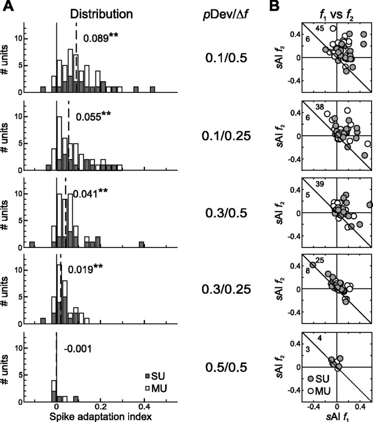
Neuronal adaptation in the awake rat A1. A, Distribution of sAIs for different stimulus conditions (indicated in the middle column; pDev/Δf) for SUs (gray bars) and MUs (white bars), with the last one (0.5/0.5) being the control condition. Median sAIs are indicated as dashed lines with the actual value printed next to it (**p < 0.01). B, Comparison of adaptation indices for f₁ and f₂ in each unit. Shown are comparisons for all stimulus configurations tested (top to bottom) and all SU recordings (gray dots) and MU recordings (white dots). There was no statistical difference between sAI for f₁ and f₂ in a given unit. In each panel, the numbers of units above versus below the drawn diagonal axis are indicated in the upper left corner.

For each unit, two sAI were calculated, separately for the lower frequency tone f₁ (sAI f₁) and the higher frequency tone f₂ (sAI f₂) to investigate asymmetries in adaptation to either of them. The vast majority of units was characterized by positive adaptation indices (Fig. 2B, points above the diagonal, indicated as numbers). This was the case for all stimulus conditions except the control condition. Any imbalance in adaptation to the lower or higher frequency would give rise to different adaptation indices sAI f₁ and sAI f₂. However, the distribution of the differences between sAI f₁ and sAI f₂ was not statistically different from 0 (signed rank test; condition 0.1/0.5: p = 0.857; condition 0.1/0.25: p = 0.074; condition 0.3/0.5: p = 0.448; condition 0.3/0.25: p = 0.688; condition 0.5/0.5: p = 0.078). In addition, there was no significant effect of unit type (single unit or multiunit) on the frequency-specific sAI (rank sum test, p > 0.05).

Time course of spike rate adaptation

The time course of adaptation during the response of a neuron to a tone was assessed by computing for each unit the difference in activity elicited by deviants and standards [difference signal (DS)]. For the stimulus condition that gave rise to the strongest adaptation (pDev = 0.1, Δf = 0.5), the mean responses (summed PSTH) of all units during stimulation with pure tone deviant stimuli and standard stimuli were compared (Fig. 3A). The average response characteristic was a transient phasic response, followed by an inhibition of activity and, after stimulus offset, a rebound in spiking activity.

Figure 3.

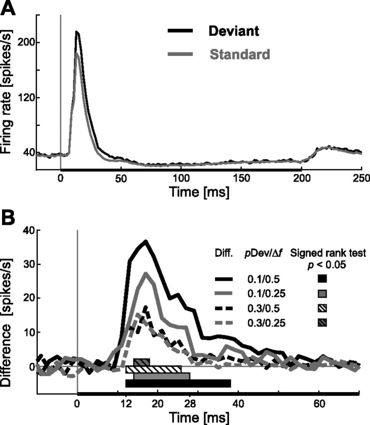
Time course of neuronal adaptation during acoustic stimulation in A1. A, Average response of 51 units during pure tone stimulation with the standard (gray line) and the deviant (black line) in a population PSTH (bin size, 2 ms; stimulus condition 0.1/0.5). Duration of the pure tone stimulus (200 ms) is indicated by a black horizontal bar below the PSTH. B, Time course of the difference signal (deviant response − standard response) from all four different stimulus configurations (i.e., 4 lines, as indicated) during the first 70 ms after stimulus onset (bin size, 2 ms). A binwise statistical comparison (signed rank test) was performed for all units for each stimulus configuration (4 populations) against a 0 distribution. Bars below the graphs indicate the period in which each difference curve was significant different from 0 (p < 0.05, Bonferroni's corrected for multiple comparisons).

The spike response to standard tones profoundly decreased relative to the response to the deviant tones within the first 50 ms after stimulus onset. After that, there was no difference observable between the two responses, in either the inhibition of activity or the rebound. Comparison of the difference signals from all four stimulus conditions (Fig. 3B) showed that the difference increased systematically with decreasing deviant probability and increasing frequency separation between the two tones, as expected from the previous results. Adaptation for all conditions, assessed binwise for each stimulus conditions (signed rank test, p < 0.05, Bonferroni's corrected for multiple comparisons) was strongest between 12 and 38 ms after stimulus onset, as indicated by bars below the difference signals (Fig. 3B). At least two difference signals differed significantly from 0 in a time window starting 12 ms after stimulus onset and lasting 16 ms until 28 ms after stimulus onset. An additional analysis was performed for these time points to see whether the deviant probability and frequency separation were significant factors controlling the amplitude of the difference signal. To this end, the means of the difference signals were computed from 12 to 28 ms after stimulus onset for each condition (condition 0.1/0.5: 27.3 spikes/s; condition 0.1/0.25: 17.1 spikes/s; condition 0.3/0.5: 9.5 spikes/s; condition 0.3/0.25: 8.6 spikes/s) and the corresponding distributions of means tested in an ANOVA [two-way ANOVA, F_(3,168) = 9.1 with pDev (p < 0.001) and Δf (p = 0.044) as factors and their interaction (p = 0.167)]. Peak latency in the mean difference signal curves was 16 ms in three cases (conditions 0.1/0.5, 0.1/0.25, and 0.3/0.5) and in one case 14 ms (condition 0.3/0.25).

To analyze the dependence of adaptation strength on stimulation history, short-term adaptation was displayed against the number of standard tones played in a row before the deviant tone (Fig. 4). During stimulus condition 0.1/0.5, deviant-related activity (normalized to the mean activity) increased by up to 34.3% when the number of standard stimuli played before increased from 0 to 5 (Fig. 4, top left panel). This increase was less pronounced for the three other stimulus conditions, but all cases revealed the same trend: the deviant response increased with the number of intersecting standard tones. After three presentations of standard stimuli, the deviant response showed the strongest increase. The mean of the deviant response after one, two, and three standard presentation was, in all but one case, >50% of the maximum activity (condition 0.1/0.5: 59.7%; condition 0.1/0.25: 57.9%; condition 0.3/0.5: 51.4%; condition 0.3/0.25: 30.2%). Therefore, the adaptation effect seems to occur mainly within the first few stimuli.

Figure 4.

Dependence of spike adaptation on the short-term stimulus history. The normalized response to deviant tones was analyzed depending on the number of standard tones presented right before. Spike activity was normalized to the mean response over all trials for one stimulus configuration. “Zero” standards means that there was deviant presented followed by a second one. Mean values from all units analyzed are given (±SEM). Activity from deviant stimuli after 10 or more standard stimuli in a row were analyzed together.

Adaptation improved neuronal discrimination of deviant stimuli

From the perspective of a neuron, one possible way for increasing the detectability (“saliency”) of low probability stimuli is to change the mean response rate to the deviant compared with the standard. This was clearly the case in the rat AC (see above), because a majority of units had positive sAIs (Fig. 2B). However, such a simple view on encoding the deviants only takes into account changes in mean spike rate but not changes in the shape of spike probability distributions. In signal detection theory, a gauge of such a change is the area under the receiver operator characteristic (AUC).

Briefly, the AUC is a measure of how well two distributions can be told apart and therefore of their discriminability. The probability distributions of spiking rates in an example neuron (Fig. 5A, left diagram) differed in response to a highly probable standard tone (p = 0.9; gray) compared with a rare deviant tone (p = 0.1; black). By simply increasing the probability of the deviant to p = 0.3, the two distributions became almost identical (Fig. 5A, middle diagram) and therefore nearly indiscriminable. These distributions (for pDev = 0.1 and pDev = 0.3) resulted in two very different ROCs and areas under ROCs (Fig. 5A, right panel). Such a change in distribution and discriminability is remarkable insofar as the frequency separation between deviant and standard in both stimulus conditions was the same (Δf = 0.5 octaves), and thus their responses derived from the tuning curve should have been very similar. The stimulus condition had a significant impact on the discriminability between deviant and standard measured as AUC for all recorded units (Fig. 5B). For every stimulus condition, the median AUC was tested against 0 and found to be significantly different, except for the control condition (signed rank test; condition 0.1/0.5: p < 0.001; condition 0.1/0.25: p < 0.001; condition 0.3/0.5: p < 0.001; condition 0.3/0.25: p < 0.001; control condition 0.5/0.5: p > 0.05). This also held true when single units and multiunits were tested separately (signed rank test, p < 0.05). There was no statistical difference between single unit and multiunit distributions (rank sum test, p > 0.05). A highly significant effect of the stimulus condition on the AUC was revealed by nonparametric ANOVA for all units (Kruskal–Wallis test, df = 4, χ² = 49.37, p < 0.001), single units (Kruskal–Wallis test, df = 4, χ² = 17.54, p = 0.001), and multiunits (Kruskal–Wallis test, df = 4, χ² = 36.56, p < 0.001). How good a measure is the adaptation index sAI for discriminating deviants from standards stimuli? There was a good correlation between the sAI of units and their area under ROC (Fig. 5C) (Spearman's rho, r_s = 0.64, p < 0.001). The correlation for the subpopulations of single units (r_s = 0.65, p < 0.001) and multiunits (r_s = 0.68, p < 0.001) were almost identical.

Figure 5.

Adaptation improves neuronal discrimination. A, Spike probability distributions for responses to standard and deviant tones from an example neuron. The left and middle panels show data from stimulation with two different stimulus condition (values for pDev and Δf are given in top right corner). Their corresponding receiver operator characteristics are depicted in the right. Numbers given along the curves in the right indicate the AUC for the two stimulus condition. B, Neuronal discrimination in A1 cortical neurons is dependent on stimulus condition. Distribution of AUC values for five different stimulus conditions are given in different panels (top to bottom, conditions as indicated). The AUC was computed from the ROC curve on the basis of the receiver operator characteristic minus 0.5 (which corresponds to 2 nonseparable distributions), giving rise to a range of possible values from −0.5 to 0.5. Values near 0 indicate nondistinguishable responses to deviant tones and standard tones. The dashed line indicates the position of the median of the AUC distribution, and the actual value is given beside the line (signed rank test, **p < 0.01). Data are shown separately for single units (gray bar) and multiunits (white bars). C, Correlation of the discriminability (measured as AUC) and the adaptation index (sAI) for each unit and for all stimulus conditions (n = 179). The Spearman's correlation coefficient r_s showed a highly significant linear correlation between these parameters (***p < 0.001, r_s value given in the panel). Single units (black dots) and multiunits (white dots) show overlapping distributions. D, Analysis of the optimal window (size and position) for pure tone signal detection by primary cortical neurons. The top two plots show the AUC encoded in grayscale depending on temporal parameters of the analysis window used. Shown are AUC values depending on the starting point (x-axis) and duration (y-axis) of the analysis window relative to stimulus onset. This examples is the same unit as shown in Figure 5A. A box plot (bottom) shows the median and range of optimal window durations for the four different stimulus conditions (stimulation parameters pDev/Δf are given on the x-axis).

Because the adaptation effect in the average difference signal was restricted to a very narrow time window (Fig. 3B), it was of interest whether there is an optimal time window and optimal window position after stimulus onset for computing the AUC and therefore for discriminating standard from deviant stimuli. The analysis of AUC with varying window durations and window positions in time relative to stimulus onset revealed a certain range of window durations and positions that were optimal in terms of discrimination between deviant and standard responses (Fig. 5D, same example as in A). The highest AUC values (0.339) at the 0.1/0.5 stimulus condition was found for a window starting 10 ms after stimulus onset and lasting 30 ms (Fig. 5D, top plot). For the 0.3/0.5 stimulus condition, the optimal window of 10 ms duration started 15 ms after stimulus onset (Fig. 5D, bottom plot), but the AUC value was low (0.04). The median of the optimal position for the analysis window in all stimulus conditions was 15 ms after stimulus onset, which matched the peak latency in the difference signal of 14–16 ms (Fig. 3B). The optimal window durations for signal detection theory shifted slightly from longer window durations to shorter durations over the stimulus conditions (from median 30 ms for condition 0.1/0.5 to a median of 20 ms for condition 0.3/0.25), but this was not significant (Kruskal–Wallis test, df = 3, χ² = 6.6, p = 0.086).

Stimulus-specific adaptation in the evoked local field potentials

To address whether SSA is present in larger neuronal ensembles, local field potentials were measured. These potentials include several signal components, for example, from the afferent pathway as well as from intracortical connections. Low-pass-filtered LFPs and high-pass-filtered spike activity were recorded simultaneously from the same electrodes to allow for a direct comparison of both signals. LFP analysis was restricted to the evoked components (eLFPs), which were manifest as a specific waveform in response to an auditory stimulus and contribute to event-related potentials recorded at even coarser spatial scales, such as EEG. The typical eLFP waveform in response to pure tones consisted of three components. Initially, there was a fast negative deflection, followed by a slower positive deflection. At the end of the stimulus, there was another negative deflection (Fig. 6, recorded simultaneously with the neuronal spike activity shown in Fig. 1C,D with the same electrode). Two components in the eLFP waveforms were analyzed: the first fast negative deflection and the slower first positive deflection. Adaptation indices for these two components (pAI–Nd and pAI–Pd, respectively) were computed on the basis of the peak negative and positive amplitudes of the mean eLFPs (see Materials and Methods). Such a procedure allowed for direct comparison of eLFP adaptation and spike adaptation (sAI). Values of pAI–Nd changed with deviant probability and frequency separation between standard and deviant stimuli (Fig. 6) in a similar way as the sAI values did (Fig. 1D). Adaptation was strong when the deviant occurred rarely (pDev = 0.1) and when the frequency separation between standard and deviant was large (Δf = 0.5 octaves). Both adaptation measures (pAI–Nd and sAI) were within a very similar range. For the pAI–Pd derived from the slower stimulus-evoked positive deflection, however, the result was different. For this component, adaptation indices were smaller than for pAI–Nd and did not vary that systematically with stimulus condition (Fig. 6).

Figure 6.

Example for adaptation in the evoked local field potentials, recorded simultaneously with the spike data (same electrode) shown in Figure 1, C and D. eLFPs to standard tones (gray line) differed mainly during response onset from eLFPs to deviant tones (black lines). The difference signal is shown as dashed line, and the stimulus is shown as black bar on the time axis. All five stimulus conditions were measured, each panel showing one condition. Two components of the response were further analyzed: the Nd and Pd as indicated in the first plot. Adaptation indices for each component (pAI–Nd and pAI-Pd) were computed on the basis of the respective peak amplitudes of the mean curves. Their values are given in the graphs.

The three components of eLFPs responses and their adaptation are more obvious in the grand means (Fig. 7A). This eLFP response pattern was well matched to the three different components of the summed spike response: phasic “on” response, inhibition, and rebound of activity (Fig. 3A). For all grand means, the deviant response was tested over the stimulus duration against the standard response (post hoc t test, p < 0.01) (p value is shown under each graph in Fig. 7A as a white line). Differences in responses to the two types of stimuli were confined to Nd in all stimulus conditions. The mean amplitude of the Nd response to standard tones was almost constant across all stimulus conditions (condition 0.1/0.5: −187 μV; condition 0.1/0.25: −191 μV; condition 0.3/0.5: −205 μV; condition 0.3/0.25: −187 μV) and did not differ significantly [two-way ANOVA, F_(3,66) = 0.57) with pDev (p = 0.42) and Δf (p = 0.7) as factors and their interaction (p = 0.74)]. The mean amplitude of the Nd responses to deviant tones seemed to change over the different stimulus conditions (condition 0.1/0.5: −235 μV; condition 0.1/0.25: −222 μV; condition 0.3/0.5: −227 μV; condition 0.3/0.25: −199 μV), but this effect was not significant [two-way ANOVA, F_(3,66) = 0.1 with pDev (p = 0.9) and Δf (p = 0.9) as factors and their interaction (p = 0.64)]. Only the differences between deviant and standard response amplitude were significant changed by deviant probability and frequency separation [two-way ANOVA, F_(3,66) = 15.5 with pDev (p < 0.001) and Δf (p = 0.006) as factors and their interaction (p = 0.46)].

Figure 7.

Grand means of eLFPs and difference signal in A1. A, Grand mean of eLFPs for standard tones (gray line) and deviant tones (black line) for all stimulus conditions (indicated at the right of the plots). Stimulation parameters are given for each panel as pDev/Δf in the column between A and B. The dashed line represents the difference signal (deviant − standard) and the black bar the stimulus (200 ms). The difference between responses to deviants and standards was tested for each time point during stimulation for statistical significance (signed rank test), and the resulting p values are plotted below the eLFPs curves as white lines with a gray background (logarithmic scale) together with the Bonferroni's level for multiple testing (white line). Maximum SEM values for the three different eLFP curves are indicated as small bars in the top right corner of each panel. B, Distribution of adaptation indices of eLFPs in the rat AC depending on stimulation condition. Adaptation indices (pAI) were calculated for each eLFP for two of its components, negative deflection (gray) and positive deflection (white), in the same way it was done for quantifying the spike adaptation. Dashed lines in histograms indicate the median of pAI–Nd, and dotted lines indicate the median of pAI–Pd (signed rank test, *p < 0.05). C, Grand mean of the difference signal of eLFPs indicates adaptation during the stimulus onset-related negative wave for all stimulus configurations. The time window in which all four difference signals are significantly different from 0 (signed rank test, **p < 0.01) is indicated by the thick black bar (including **) above the four curves and as values on the time axis (15–29 ms). Stimulus duration is indicated by the horizontal bar at the bottom. Stimulation parameters for each curve are given as pDev/Δf.

Unlike responses of single neurons, eLFPs adapted not only in the first, fast response (Nd) but also in the second, slower component (Pd). However, the adaptation in Pd was less systematic and weaker than in Nd. As in the spike data, median adaptation indices of Nd varied with deviant probability and frequency separation (Fig. 7B). Only the distribution of pAI–Nd was statistically different from 0 in all four stimulus condition (median and signed rank test; condition 0.1/0.5: 0.1, p < 0.001; condition 0.1/0.25: 0.055, p < 0.001; condition 0.3/0.5: 0.043, p = 0.004; condition 0.3/0.25: 0.035, p < 0.001; control condition 0.5/0.5: −0.013, p = 0.844), and an ANOVA showed a significant effect of stimulus condition on pAI–Nd (Kruskal–Wallis test, df = 4, χ² = 26.43, p < 0.001). There was an effect of stimulus condition on pAI–Pd as well, but it was less systematic (median and signed rank test; condition 0.1/0.5: 0.102, p = 0.001; condition 0.1/0.25: 0.063, p = 0.002; condition 0.3/0.5: 0.01, p = 0.375; condition 0.3/0.25: 0.01, p = 0.174; control condition 0.5/0.5: −0.027, p = 0.219).

This difference between Nd and Pd was more obvious in the difference signal (deviant − standard) (Fig. 7C). For all four stimulus conditions, a significant Nd difference amplitude was found (post hoc t test, nondirectional, p < 0.01; indicated by the horizontal bar with asterisk above the graphs). The temporal range of maximum difference covered only a short span of 14 ms (from 15 to 29 ms after stimulus onset), which was almost identical to the significant spike difference signal (Fig. 3B, 12–28 ms). Peak latencies of the mean negative difference signals were 25 ms (condition 0.1/0.5), 26 ms (condition 0.1/0.25), 25 ms (condition 0.3/0.5), and 23 ms (condition 0.3/0.25). Adaptation in the positive eLFP deflection Pd was less clear. There was a difference in response to standard tones compared with deviant tones that was significant (Fig. 7A, first three panels) but only for stimulus conditions that gave rise to strong adaptation in the negative deflection as well. Differences in Pd amplitude were not as systematically ordered as was the case for Nd amplitude. It has to be emphasized that the negative component of the difference signal was not attributable to a change in signs for the standard eLFP while the deviant eLFP remained negative but solely to an increased negative amplitude of the deviant eLFP. In addition, we note that there was a prominent “off” component in the eLFPs after stimulus offset that was only marginally present in simultaneously recorded spike activity (compare Figs. 1D, 3A). This component showed no adaptation to the standard and was not affected by stimulus condition, hinting toward additional factors contributing to eLFP signal compared with spike responses. All adaptation indices calculated for this late eLFP component at stimulus offset (200–300 ms after stimulus onset) were not significantly different from 0 (signed rank test; condition 0.1/0.5: p = 0.078; condition 0.1/0.25: p = 0.31; condition 0.3/0.5: p = 0.13; condition 0.3/0.25: p = 0.57; condition 0.5/0.5: p = 0.15), nor was there a significant effect of stimulus condition on this pAI (Kruskal–Wallis test, df = 4, χ² = 5.68, p = 0.22).

A stimulus omission elicited no change in neuronal activity

To exclude that the shown effects are attributable to a mere change in the sequence of expected repetitive stimuli, we substituted the deviant with a stimulus omission of the same duration (200 ms). All other parameters were identical to stimulus condition 0.1/0.5. For this experiment, units with a high level of interstimulus activity (“spontaneous activity”) were selected because they allow to study both excitatory and inhibitory effects. During stimulus omission, interstimulus spike activity and eLFPs did not change. In summary, there was no adaptation-like effect of stimulus omission in an otherwise constant sequence of pure tones at a repetition rate of 1 Hz in the awake rat A1.

Correlation between spike adaptation and eLFP adaptation

To assess the relationship between the spike adaptation shown so far and the adaptation present in the eLFPs, a correlation analysis was performed for simultaneously recorded datasets of both types of signals (Fig. 8). For each stimulus condition, the Spearman's rank correlation coefficient (r_s) was computed for sAI versus pAI–Nd and sAI versus pAI–Pd. There was a tight correlation between sAI and pAI–Nd for all four stimulus conditions (rank correlation; condition 0.1/0.5: p = 0.002; condition 0.1/0.25: p = 0.0023; condition 0.3/0.5: p < 0.001; condition 0.3/0.25: p = 0.009) but not the control (condition 0.5/0.5: p = 0.62). This was not the case for adaptation indices calculated for the positive deflection pAI–Pd (condition 0.1/0.5: p = 0.13; condition 0.1/0.25: p = 0.91; condition 0.3/0.5: p = 0.58; condition 0.3/0.25: p = 0.11; condition 0.5/0.5: p = 0.79). For sAI versus pAI–Nd, the rank correlation coefficient r_s with sAI was always larger than for sAI versus pAI–Pd. This very consistent correlation pattern indicates that there is close relationship between spike adaptation and the first negative deflection of eLFPs.

Figure 8.

Correlation of adaptation between spiking response and eLFPs. For a certain number of units, eLFPs were recorded in parallel and allowed for comparison of their respective adaptation indices. This was done for all four stimulus conditions (from left to right, pDev/Δf). The top row shows spike adaptation versus eLFP adaptation of the negative deflection, and the bottom row shows sAI versus eLFP adaptation of the positive deflection. For each stimulus condition, a correlation analysis was done between sAI and pAI. All correlations were tested nonparametrically (Spearman's rho), and test results are shown in each plot (**p < 0.01).

Latencies of the spike and eLFP response

To clarify the temporal relationship between adaptation present in spikes and eLFPs, it is important to compare their respective latencies (Fig. 9). There was a significant effect of stimulus condition on neither response latency of the spike difference signal (Kruskal–Wallis test, df = 3, χ² = 1.88, p = 0.6) (see also Fig. 3B) nor the latency of the Nd difference signal (Kruskal–Wallis test, df = 3, χ² = 4.74, p = 0.19) (compare with Fig. 7C) or the Pd difference signal (Kruskal–Wallis test, df = 3, χ² = 5.73, p = 0.12) (Fig. 7C). Median latencies of both responses (spike, 16 ms; Nd, 22 ms) were well matched by peak latencies of the difference signal (spike DS: 16, 16, 16, and 14 ms; Nd DS: 25, 26, 25, and 23 ms). There was no statistical difference in the latencies of responses to standard tones and deviant tones for any stimulus condition for neither the spike response (rank sum test, p > 0.1), eLFP–Nd (rank sum test, p > 0.1), nor eLFP–Pd (rank sum test, p > 0.1). The latency difference between spike responses and eLFP responses could be a consequence of the hardware filter applied during the recordings.

Figure 9.

Latencies of the isolated units and eLFPs peak negative deflection. Distribution of peak latencies of spikes (1 ms resolution) and eLFPs negative deflection, separated for deviants and standards. The spike latencies were computed as the bin with maximum response in the PSTH and the eLFP latencies as the sample point with the lowest amplitude. There is no statistical difference between any of the deviant–standard combinations and no effect of stimulus configuration.

To ensure that small latency differences between deviant and standard responses were not masked by the high variability of absolute latencies, we further analyzed latency differences between deviant and standard responses for each unit and eLFP–Nd recording. The median of the differences (deviant latency − standard latency) was exactly 0 for both spike response latency and eLFP–Nd response latency. For all except one stimulus condition, the median of these differences was statistically not different from 0 for spike latencies (signed rank test; all conditions, p > 0.05, corrected for multiple testing) and eLFP–Nd latencies (signed rank test; condition 0.1/0.5: p = 0.01; all other conditions: p > 0.05, corrected for multiple testing).

Histological confirmation of recording sites

After finishing the recordings in an animal, the recording sites were reconstructed based on electrolytic lesions and histological staining of coronal brain sections. The lesions were set at two positions: the depth of the last and the first recording site. For each animal, the cortical region and laminar position of the lesion was reconstructed and compared with A1 (Paxinos and Watson, 1998) and to the field Te1 (Zilles, 1985), respectively (Fig. 10). For all eight animals in this study, the recordings sites were confirmed to be in A1. The laminar reconstruction of recording sites varied between layer III and V, with majority of sites being in layers IV–V (animal 31, layer IV; animal 34, layer V; animal 41, layer V; animal 42, layer III; animal 48, layer V; animal 51, layer IV; animal 52, layer V; animal 57, layer III). The median adaptation indices spikes (sAI) for different layers were 0.065 (layer III), 0.033 (layer IV), and 0.04 (layer V) and for LFPs (pAI–Nd) were 0.052 (layer III), 0.042 (layer IV), and 0.044 (layer V). There was no significant effect of the layer (layers III–V) on neither sAI (Kruskal–Wallis test, df = 2, χ² = 1.32, p = 0.516) nor pAI–Nd (Kruskal–Wallis test, df = 2, χ² = 4.17, p = 0.124). Furthermore, the individual animal was no significant factor influencing sAI (Kruskal–Wallis test, df = 7, χ² = 12.46, p = 0.085) or pAI–Nd (Kruskal–Wallis test, df = 3, χ² = 4.92, p = 0.177) .

Figure 10.

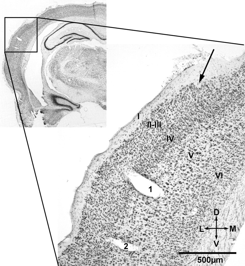
Histological reconstruction of recording sites. Example of the histological reconstruction of recordings sites in one animal. The inset at the top left side shows the left hemisphere with the region of higher magnification indicated by a black frame. The magnified coronal section (50 μm thick; scale bar, 500 μm) shows the electrolytic lesions of one electrode track in the primary auditory cortex [according to Paxinos and Watson (1998) at ∼6 mm caudal from bregma]. Lesions were performed after finishing the experiments at the site of the first recording (marked with 1) and the last recording (marked with 2) in a tangential approach. The arrow at the top right side shows the penetration site of the electrode into the cortex. Additionally, the cortical layers are indicated (according to Zilles, 1985) in roman numbers.

Discussion

This study investigated, with an oddball paradigm, neuronal adaptation in A1 of the awake rat at the level of isolated units and eLFPs. The main findings were as follows. (1) Isolated units in A1 of the awake rat showed SSA primarily during the onset response but could not be observed during later inhibition or rebound of activity. SSA of isolated units depended on at least two factors: frequency separation and the deviant probability. However, SSA was independent of the specific frequency (f₁ or f₂), indicating that SSA might be a more general property of cortical neurons. (2) Certain components of eLFPs adapted in a stimulus-specific manner (i.e., the fast negative deflection and partially the slower positive deflection). There was, however, no MMN response present. (3) Spike adaptation correlated well with the adaptation of Nd but not Pd. Adaptation of Nd resembled spike adaptation with respect to magnitude and dependency on Δf and pDev.

Role of cortical state

Most of the recent studies investigating adaptation at the level of single neurons were done in anesthetized animals, e.g., rats (Pérez-González et al., 2005; Malmierca et al., 2009), guinea pigs (Dean et al., 2005, 2008) or cats (Ulanovsky et al., 2003, 2004). These studies found on average stronger adaptation effects than the ones presented here but are hard to compare because of the differences in animal model, brain region, and paradigm. Furthermore, one has to consider the interstimulus interval (ISI) (onset to onset) of 1000 ms applied here, which is in the typical range of many MMN studies (Javitt et al., 1992; Sussman et al., 1998; Jemel et al., 2002) but rather slow compared with other SSA studies (Ulanovsky et al., 2003: ISI of 375–4000 ms; Anderson et al., 2009: ISI of 400–800 ms; Malmierca et al., 2009: ISI of 125–500 ms). It is reasonable to expect bigger effects at smaller ISIs, as was shown previously for neurons in the auditory cortex (Ulanovsky et al., 2003) and MMN (Sabri and Campbell, 2001).

However, another hypothesis would be that the difference also might be attributable to the effects of anesthetics. It has been shown in rat AC that, under anesthesia, there is larger decrease in multiunit response during a sequence of clicks compared with the awake state (Rennaker et al., 2007). The AC is very susceptible to anesthesia. Response properties of A1 neurons in rodent are changed profoundly by application of Equithesin, urethane, or ketamine (Gaese and Ostwald, 2001; Cotillon-Williams and Edeline, 2003; Syka et al., 2005). Different anesthetics can exert a variety of effects on auditory cortical neurons resulting in, for example, threshold changes (Cheung et al., 2001), altered spontaneous rate (Zurita et al., 1994), or evoked oscillations (Cotillon-Williams and Edeline, 2003). This holds true not only for single neuron activity but also for evoked auditory potentials in rats (Borbély and Hall, 1970; Kisley and Gerstein, 1999; Miyazato et al., 1999). Similar studies performed in awake animals (Condon and Weinberger, 1991; Malone et al., 2002; Brosch and Scheich, 2008) apply paradigms with different timescales and therefore are difficult to compare with the typical oddball paradigm used for SSA and MMN.

Pattern and origin of spike and eLFP adaptation

Adaptation of spike responses and eLFPs as shown here was a phenomenon present only within a short time window of a few milliseconds after stimulus onset. In the eLFPs, the slower positive deflection showed adaptation as well but was less pronounced. The very phasic response patterns in both Nd and spikes are characteristic for A1 of the rat (Borbély, 1970; DeWeese et al., 2003), determining strongly the temporal structure of adaptation, as in our case during the onset but not the following inhibition or rebound of activity. As demonstrated by Wang et al. (2005), the response pattern in the awake AC depends critically on the nature of the stimulus. Because neurons in the rat A1 are capable of representing a wide range of temporally and spectrally dynamic stimuli (Zhang et al., 2003; Hromádka et al., 2008), it is likely that there are other stimuli evoking more tonic responses. The recorded eLFPs are characteristic for the rat AC and correspond to layers IV–V (Borbély, 1970; Barth and Di, 1990), which matches our histological reconstruction and the spike response patterns found in layer V pyramidal neurons (Hefti and Smith, 2000). The LFP signal is the weighted averaged of the negative time derivative of coherent postsynaptic excitatory potentials of mostly cortical pyramidal cells (Creutzfeldt et al., 1966; Kaur et al., 2004; Burkhard et al., 2006). Postsynaptic depolarization is therefore measured as a negative wave in the eLFPs paralleled by an increased spike rate (Destexhe et al., 1999). Therefore, eLFPs are good predictors for spike occurrence (Eggermont and Smith, 1995; Rasch et al., 2008). The first negative deflection in the rat A1 layers IV–V stems from a current sink and can be accounted for mainly by apical dendrites of pyramidal cells in supragranular and infragranular layers (Barth and Di, 1990; Sukov and Barth, 1998). A conservative estimate for the spatial origin of LFPs is in the range of ≤1 mm (rat AC: Kaur et al., 2004), but recently a study gauged this distance at ∼250 μm (cat visual cortex: Katzner et al., 2009).

Different networks contribute to the eLFPs

Our results show a close correlation between eLFP fast negative deflection adaptation and spike adaptation (Fig. 8, top row), whereas the adaptation of the slower eLFP positive deflection has no complement in the spike response. We think that there is a strong contribution of the very local circuitry to the eLFP fast negative deflection, which strongly influences isolated neurons as well as the summed potentials. One aspect could be a layer specificity of adaptation, as was shown for MMN in the primate AC (Javitt et al., 1994). In the rat AC, the first intracortical negative wave matches with the first epidural positive wave (P1) (Barth and Di, 1990). The timing of LFP components depends, however, on cortical depth, and, therefore, the epicortical waves cannot be matched directly to LFP components. We consider the first negative wave in our eLFP recordings to contribute to P1/N1 complex because of the matching latencies [Fig. 9, compare with Ohl et al. (2000) and Barth and Di (1990)]. Following the same reasoning, the slower positive wave contributes to the P2/N2 complex.

In rat AC, the fast P1/N1 complex presumably has a focal topology and may reflect cortical responses to stimulus-specific and spectrally selective thalamocortical input, whereas the slower waves P2/N2 depend on more widespread corticocortical connections (Shaw, 1988; Barth and Di, 1990; Brett et al., 1996). This spatial dichotomy between the fast and slow waves is supported by Barth et al. (1993) and Ohl et al. (2000), who both showed that fast P1 and N1 are centered in A1 and that slow P2 and N2 originate in A1 plus secondary AC. We suspect that adaptation in rat A1 reflects properties of the thalamocortical projections because we saw a good correlation between spike adaptation and adaptation of the fast Nd. The adaptation of the slower Pd did not correlate with spiking activity and therefore seemed to originate from a different source such as a corticocortical network.

Adaptation without MMN in A1

Single neuron and LFP adaptation phenomena (i.e., SSA) are a presumed neuronal basis of the MMN. One of the hallmarks of MMN is the dependency on the deviance and probability of the deviant, just as we have shown it for the adaptation of spike activity and eLFPs. The origin of MMN is still a matter of debate. There are few rodent studies approaching MMN generation by means of event-related potentials, but, so far, the results show no unequivocal pattern (Nelken and Ulanovsky, 2007). Here we show that there is deviant-related adaptation of activity in the rat A1 at the level of isolated units and eLFPs. Although we could demonstrate that adaptation improves neuronal discrimination (Fig. 5), the characteristics of this adaptation does not match those of human MMN or of MMN demonstrated for cat (Pincze et al., 2001) and monkeys (Javitt et al., 1992, 1994, 1996). Rather, it seems as if spike adaptation contributed profoundly to a change in amplitude of the P1/N1 complex but could not be related to the slower P2/N2 complex. The N1 wave amplitude of human EEG is susceptible to frequency deviants probably by recruiting new afferent elements (Näätänen et al., 1988). Thus, spike adaptation and the correlating changes in the eLFPs negative deflection, which corresponds to N1, may contribute to a larger network for sound discrimination, which ultimately is the foundation of MMN.

It has been argued that MMN is attributable to changes in N1 subcomponents [adaptation hypothesis (Jääskeläinen et al., 2004)] and not to a change-specific memory-based response, as has been postulated by Näätänen et al. (2005). From our results, we conclude that SSA of isolated units in rat A1 contribute to changes in the N1/P1 complex. However, adaptation of eLFPs can occur without the response characteristics of MMN. Later changes in the eLFP response (Pd) are not directly related to the adaptation present in spikes in terms of neither latency nor magnitude. However, it resembled repetition positivity, which is discussed as a contributor to MMN (Haenschel et al., 2005). The absence of MMN could be attributable to either the chosen animal model or the cortical region from which we recorded. For the cat and guinea pig, it has been shown that MMN is generated in the nonprimary auditory pathway (Kraus et al., 1994; Pincze et al., 2001). Only a systematic comparison of different auditory fields and different species could resolve this question.

References

- Anderson LA, Christianson GB, Linden JF. Stimulus-specific adaptation occurs in the auditory thalamus. J Neurosci. 2009;29:7359–7363. doi: 10.1523/JNEUROSCI.0793-09.2009. [DOI] [PMC free article] [PubMed] [Google Scholar]
- Astikainen P, Ruusuvirta T, Wikgren J, Penttonen M. Memory-based detection of rare sound feature combinations in anesthetized rats. Neuroreport. 2006;17:1561–1564. doi: 10.1097/01.wnr.0000233097.13032.7d. [DOI] [PubMed] [Google Scholar]
- Barlow HB, Levick WR, Yoon M. Responses to single quanta of light in retinal ganglion cells of the cat. Vision Res. 1971;3(Suppl):87–101. doi: 10.1016/0042-6989(71)90033-2. [DOI] [PubMed] [Google Scholar]
- Barth DS, Di S. Three-dimensional analysis of auditory-evoked potentials in rat neocortex. J Neurophysiol. 1990;64:1527–1536. doi: 10.1152/jn.1990.64.5.1527. [DOI] [PubMed] [Google Scholar]
- Barth DS, Kithas J, Di S. Anatomic organization of evoked potentials in rat parietotemporal cortex: somatosensory and auditory responses. J Neurophysiol. 1993;69:1837–1849. doi: 10.1152/jn.1993.69.6.1837. [DOI] [PubMed] [Google Scholar]
- Borbély AA. Changes in click-evoked responses as a function of depth in auditory cortex of the rat. Brain Res. 1970;21:217–247. doi: 10.1016/0006-8993(70)90365-3. [DOI] [PubMed] [Google Scholar]
- Borbély AA, Hall RD. Effects of pentobarbitone and chlorpromazine on acoustically evoked potentials in the rat. Neuropharmacology. 1970;9:575–586. doi: 10.1016/0028-3908(70)90008-0. [DOI] [PubMed] [Google Scholar]
- Bregman AS. Auditory scene analysis: the perceptual organization of sound. Cambridge, MA: MIT; 1990. [Google Scholar]
- Brenner N, Bialek W, de Ruyter van Steveninck R. Adaptive rescaling maximizes information transmission. Neuron. 2000;26:695–702. doi: 10.1016/s0896-6273(00)81205-2. [DOI] [PubMed] [Google Scholar]
- Brett B, Krishnan G, Barth DS. The effects of subcortical lesions on evoked potentials and spontaneous high frequency (gamma-band) oscillating potentials in rat auditory cortex. Brain Res. 1996;721:155–166. doi: 10.1016/0006-8993(96)00168-0. [DOI] [PubMed] [Google Scholar]
- Brosch M, Scheich H. Tone-sequence analysis in the auditory cortex of awake macaque monkeys. Exp Brain Res. 2008;184:349–361. doi: 10.1007/s00221-007-1109-7. [DOI] [PubMed] [Google Scholar]
- Burkhard RF, Don M, Eggermont JJ, editors. Auditory evoked potentials: basic principles and clinical application. Baltimore: Lippencott Williams and Wilkins; 2006. [Google Scholar]
- Cheung SW, Nagarajan SS, Bedenbaugh PH, Schreiner CE, Wang X, Wong A. Auditory cortical neuron response differences under isoflurane versus pentobarbital anesthesia. Hear Res. 2001;156:115–127. doi: 10.1016/s0378-5955(01)00272-6. [DOI] [PubMed] [Google Scholar]
- Condon CD, Weinberger NM. Habituation produces frequency-specific plasticity of receptive fields in the auditory cortex. Behav Neurosci. 1991;105:416–430. doi: 10.1037//0735-7044.105.3.416. [DOI] [PubMed] [Google Scholar]
- Cotillon-Williams N, Edeline JM. Evoked oscillations in the thalamo-cortical auditory system are present in anesthetized but not in unanesthetized rats. J Neurophysiol. 2003;89:1968–1984. doi: 10.1152/jn.00728.2002. [DOI] [PubMed] [Google Scholar]
- Creutzfeldt OD, Watanabe S, Lux HD. Relations between EEG phenomena and potentials of single cortical cells. I. Evoked responses after thalamic and epicortical stimulation. Electroencephalogr Clin Neurophysiol. 1966;20:1–18. doi: 10.1016/0013-4694(66)90136-2. [DOI] [PubMed] [Google Scholar]
- Dean I, Harper NS, McAlpine D. Neural population coding of sound level adapts to stimulus statistics. Nat Neurosci. 2005;8:1684–1689. doi: 10.1038/nn1541. [DOI] [PubMed] [Google Scholar]
- Dean I, Robinson BL, Harper NS, McAlpine D. Rapid neural adaptation to sound level statistics. J Neurosci. 2008;28:6430–6438. doi: 10.1523/JNEUROSCI.0470-08.2008. [DOI] [PMC free article] [PubMed] [Google Scholar]
- Destexhe A, Contreras D, Steriade M. Spatiotemporal analysis of local field potentials and unit discharges in cat cerebral cortex during natural wake and sleep states. J Neurosci. 1999;19:4595–4608. doi: 10.1523/JNEUROSCI.19-11-04595.1999. [DOI] [PMC free article] [PubMed] [Google Scholar]
- DeWeese MR, Wehr M, Zador AM. Binary spiking in auditory cortex. J Neurosci. 2003;23:7940–7949. doi: 10.1523/JNEUROSCI.23-21-07940.2003. [DOI] [PMC free article] [PubMed] [Google Scholar]
- Eggermont JJ, Smith GM. Synchrony between single-unit activity and local field potentials in relation to periodicity coding in primary auditory cortex. J Neurophysiol. 1995;73:227–245. doi: 10.1152/jn.1995.73.1.227. [DOI] [PubMed] [Google Scholar]
- Eriksson J, Villa AEP. Event-related potentials in an auditory oddball situation in the rat. Biosystems. 2005;79:207–212. doi: 10.1016/j.biosystems.2004.09.017. [DOI] [PubMed] [Google Scholar]
- Escera C, Alho K, Winkler I, Näätänen R. Neural mechanisms of involuntary attention to acoustic novelty and change. J Cogn Neurosci. 1998;10:590–604. doi: 10.1162/089892998562997. [DOI] [PubMed] [Google Scholar]
- Frank LM, Brown EN, Wilson MA. A comparison of the firing properties of putative excitatory and inhibitory neurons from CA1 and the entorhinal cortex. J Neurophysiol. 2001;86:2029–2040. doi: 10.1152/jn.2001.86.4.2029. [DOI] [PubMed] [Google Scholar]
- Gaese BH, Ostwald J. Anesthesia changes frequency tuning of neurons in the rat primary auditory cortex. J Neurophysiol. 2001;86:1062–1066. doi: 10.1152/jn.2001.86.2.1062. [DOI] [PubMed] [Google Scholar]
- Giard MH, Lavikahen J, Reinikainen K, Perrin F, Bertrand O, Pernier J, Näätänen R. Separate representation of stimulus frequency, intensity, and duration in auditory sensory memory: an event-related potential and dipole-model analysis. J Cogn Neurosci. 1995;7:133–143. doi: 10.1162/jocn.1995.7.2.133. [DOI] [PubMed] [Google Scholar]
- Haenschel C, Vernon DJ, Dwivedi P, Gruzelier JH, Baldeweg T. Event-related brain potential correlates of human auditory sensory memory-trace formation. J Neurosci. 2005;25:10494–10501. doi: 10.1523/JNEUROSCI.1227-05.2005. [DOI] [PMC free article] [PubMed] [Google Scholar]
- Hefti BJ, Smith PH. Anatomy, physiology, and synaptic responses of rat layer v auditory cortical cells and effects of intracellular GABAA blockade. J Neurophysiol. 2000;83:2626–2638. doi: 10.1152/jn.2000.83.5.2626. [DOI] [PubMed] [Google Scholar]
- Hromádka T, Deweese MR, Zador AM. Sparse representation of sounds in the unanesthetized auditory cortex. PLoS Biol. 2008;6:e16. doi: 10.1371/journal.pbio.0060016. [DOI] [PMC free article] [PubMed] [Google Scholar]
- Jääskeläinen IP, Ahveninen J, Bonmassar G, Dale AM, Ilmoniemi RJ, Levänen S, Lin FH, May P, Melcher J, Stufflebeam S, Tiitinen H, Belliveau JW. Human posterior auditory cortex gates novel sounds to consciousness. Proc Natl Acad Sci U S A. 2004;101:6809–6814. doi: 10.1073/pnas.0303760101. [DOI] [PMC free article] [PubMed] [Google Scholar]
- Javitt DC, Schroeder CE, Steinschneider M, Arezzo JC, Vaughan HG., Jr Demonstration of mismatch negativity in the monkey. Electroencephalogr Clin Neurophysiol. 1992;83:87–90. doi: 10.1016/0013-4694(92)90137-7. [DOI] [PubMed] [Google Scholar]
- Javitt DC, Steinschneider M, Schroeder CE, Vaughan HG, Jr, Arezzo JC. Detection of stimulus deviance within primate primary auditory cortex: intracortical mechanisms of mismatch negativity (MMN) generation. Brain Res. 1994;667:192–200. doi: 10.1016/0006-8993(94)91496-6. [DOI] [PubMed] [Google Scholar]
- Javitt DC, Steinschneider M, Schroeder CE, Arezzo JC. Role of cortical N-methyl-d-aspartate receptors in auditory sensory memory and mismatch negativity generation: implications for schizophrenia. Proc Natl Acad Sci U S A. 1996;93:11962–11967. doi: 10.1073/pnas.93.21.11962. [DOI] [PMC free article] [PubMed] [Google Scholar]
- Jemel B, Achenbach C, Müller BW, Röpcke B, Oades RD. Mismatch negativity results from bilateral asymmetric dipole sources in the frontal and temporal lobes. Brain Topogr. 2002;15:13–27. doi: 10.1023/a:1019944805499. [DOI] [PubMed] [Google Scholar]
- Katzner S, Nauhaus I, Benucci A, Bonin V, Ringach DL, Carandini M. Local origin of field potentials in visual cortex. Neuron. 2009;61:35–41. doi: 10.1016/j.neuron.2008.11.016. [DOI] [PMC free article] [PubMed] [Google Scholar]
- Kaur S, Lazar R, Metherate R. Intracortical pathways determine breadth of subthreshold frequency receptive fields in primary auditory cortex. J Neurophysiol. 2004;91:2551–2567. doi: 10.1152/jn.01121.2003. [DOI] [PubMed] [Google Scholar]
- Kisley MA, Gerstein GL. Trial-to-trial variability and state-dependent modulation of auditory-evoked responses in cortex. J Neurosci. 1999;19:10451–10460. doi: 10.1523/JNEUROSCI.19-23-10451.1999. [DOI] [PMC free article] [PubMed] [Google Scholar]
- Kraus N, McGee T, Littman T, Nicol T, King C. Nonprimary auditory thalamic representation of acoustic change. J Neurophysiol. 1994;72:1270–1277. doi: 10.1152/jn.1994.72.3.1270. [DOI] [PubMed] [Google Scholar]
- Kvale MN, Schreiner CE. Short-term adaptation of auditory receptive fields to dynamic stimuli. J Neurophysiol. 2004;91:604–612. doi: 10.1152/jn.00484.2003. [DOI] [PubMed] [Google Scholar]
- Lazar R, Metherate R. Spectral interactions, but no mismatch negativity, in auditory cortex of anesthetized rat. Hear Res. 2003;181:51–56. doi: 10.1016/s0378-5955(03)00166-7. [DOI] [PubMed] [Google Scholar]
- Malmierca MS, Cristaudo S, Pérez-González D, Covey E. Stimulus-specific adaptation in the inferior colliculus of the anesthetized rat. J Neurosci. 2009;29:5483–5493. doi: 10.1523/JNEUROSCI.4153-08.2009. [DOI] [PMC free article] [PubMed] [Google Scholar]
- Malone BJ, Scott BH, Semple MN. Context-dependent adaptive coding of interaural phase disparity in the auditory cortex of awake macaques. J Neurosci. 2002;22:4625–4638. doi: 10.1523/JNEUROSCI.22-11-04625.2002. [DOI] [PMC free article] [PubMed] [Google Scholar]
- Miyazato H, Skinner RD, Cobb M, Andersen B, Garcia-Rill E. Midlatency auditory-evoked potentials in the rat: effects of interventions that modulate arousal. Brain Res Bull. 1999;48:545–553. doi: 10.1016/s0361-9230(99)00034-9. [DOI] [PubMed] [Google Scholar]
- Näätänen R, Gaillard AW, Mäntysalo S. Early selective-attention effect on evoked potential reinterpreted. Acta Psychol (Amst) 1978;42:313–329. doi: 10.1016/0001-6918(78)90006-9. [DOI] [PubMed] [Google Scholar]
- Näätänen R, Sams M, Alho K, Paavilainen P, Reinikainen K, Sokolov EN. Frequency and location specificity of the human vertex N1 wave. Electroencephalogr Clin Neurophysiol. 1988;69:523–531. doi: 10.1016/0013-4694(88)90164-2. [DOI] [PubMed] [Google Scholar]
- Näätänen R, Jacobsen T, Winkler I. Memory-based or afferent processes in mismatch negativity (MMN): a review of the evidence. Psychophysiology. 2005;42:25–32. doi: 10.1111/j.1469-8986.2005.00256.x. [DOI] [PubMed] [Google Scholar]
- Näätänen R, Paavilainen P, Rinne T, Alho K. The mismatch negativity (MMN) in basic research of central auditory processing: a review. Clin Neurophysiol. 2007;118:2544–2590. doi: 10.1016/j.clinph.2007.04.026. [DOI] [PubMed] [Google Scholar]
- Nelken I, Ulanovsky N. Mismatch negativity and simulus-specific adaptation in animal models. J Psychophysiol. 2007;21:214–223. [Google Scholar]
- Ohl FW, Scheich H, Freeman WJ. Topographic analysis of epidural pure-tone-evoked potentials in gerbil auditory cortex. J Neurophysiol. 2000;83:3123–3132. doi: 10.1152/jn.2000.83.5.3123. [DOI] [PubMed] [Google Scholar]
- Paxinos G, Watson C. The rat brain in stereotaxic coordinates. London: Academic; 1998. [DOI] [PubMed] [Google Scholar]
- Pérez-González D, Malmierca MS, Covey E. Novelty detector neurons in the mammalian auditory midbrain. Eur J Neurosci. 2005;22:2879–2885. doi: 10.1111/j.1460-9568.2005.04472.x. [DOI] [PubMed] [Google Scholar]
- Pincze Z, Lakatos P, Rajkai C, Ulbert I, Karmos G. Separation of mismatch negativity and the N1 wave in the auditory cortex of the cat: a topographic study. Clin Neurophysiol. 2001;112:778–784. doi: 10.1016/s1388-2457(01)00509-0. [DOI] [PubMed] [Google Scholar]
- Rasch MJ, Gretton A, Murayama Y, Maass W, Logothetis NK. Inferring spike trains from local field potentials. J Neurophysiol. 2008;99:1461–1476. doi: 10.1152/jn.00919.2007. [DOI] [PubMed] [Google Scholar]
- Rennaker RL, Carey HL, Anderson SE, Sloan AM, Kilgard MP. Anesthesia suppresses nonsynchronous responses to repetitive broadband stimuli. Neuroscience. 2007;145:357–369. doi: 10.1016/j.neuroscience.2006.11.043. [DOI] [PubMed] [Google Scholar]
- Rutkowski RG, Miasnikov AA, Weinberger NM. Characterisation of multiple physiological fields within the anatomical core of rat auditory cortex. Hear Res. 2003;181:116–130. doi: 10.1016/s0378-5955(03)00182-5. [DOI] [PubMed] [Google Scholar]
- Ruusuvirta T, Penttonen M, Korhonen T. Auditory cortical event-related potentials to pitch deviances in rats. Neurosci Lett. 1998;248:45–48. doi: 10.1016/s0304-3940(98)00330-9. [DOI] [PubMed] [Google Scholar]
- Sabri M, Campbell KB. Effects of sequential and temporal probability of deviant occurrence on mismatch negativity. Brain Res Cogn Brain Res. 2001;12:171–180. doi: 10.1016/s0926-6410(01)00026-x. [DOI] [PubMed] [Google Scholar]
- Sambeth A, Maes JH, Van Luijtelaar G, Molenkamp IB, Jongsma ML, Van Rijn CM. Auditory event-related potentials in humans and rats: effects of task manipulation. Psychophysiology. 2003;40:60–68. doi: 10.1111/1469-8986.00007. [DOI] [PubMed] [Google Scholar]
- Schröger E. The influence of stimulus intensity and inter-stimulus interval on the detection of pitch and loudness changes. Electroencephalogr Clin Neurophysiol. 1996;100:517–526. [PubMed] [Google Scholar]
- Shaw NA. The auditory evoked potential in the rat: a review. Prog Neurobiol. 1988;31:19–45. doi: 10.1016/0301-0082(88)90021-4. [DOI] [PubMed] [Google Scholar]
- Stüttgen MC, Schwarz C. Psychophysical and neurometric detection performance under stimulus uncertainty. Nat Neurosci. 2008;11:1091–1099. doi: 10.1038/nn.2162. [DOI] [PubMed] [Google Scholar]
- Sukov W, Barth DS. Three-dimensional analysis of spontaneous and thalamically evoked gamma oscillations in auditory cortex. J Neurophysiol. 1998;79:2875–2884. doi: 10.1152/jn.1998.79.6.2875. [DOI] [PubMed] [Google Scholar]
- Sussman E, Ritter W, Vaughan HG., Jr Predictability of stimulus deviance and the mismatch negativity. Neuroreport. 1998;9:4167–4170. doi: 10.1097/00001756-199812210-00031. [DOI] [PubMed] [Google Scholar]
- Sussman ES. A new view on the MMN and attention debate: the role of context in processing auditory events. J Psychophysiol. 2007;3–4:164–175. [Google Scholar]
- Syka J, Suta D, Popelár J. Responses to species-specific vocalizations in the auditory cortex of awake and anesthetized guinea pigs. Hear Res. 2005;206:177–184. doi: 10.1016/j.heares.2005.01.013. [DOI] [PubMed] [Google Scholar]
- Tikhonravov D, Neuvonen T, Pertovaara A, Savioja K, Ruusuvirta T, Näätänen R, Carlson S. Effects of an NMDA-receptor antagonist MK-801 on an MMN-like response recorded in anesthetized rats. Brain Res. 2008;1203:97–102. doi: 10.1016/j.brainres.2008.02.006. [DOI] [PubMed] [Google Scholar]
- Ulanovsky N, Las L, Nelken I. Processing of low-probability sounds by cortical neurons. Nat Neurosci. 2003;6:391–398. doi: 10.1038/nn1032. [DOI] [PubMed] [Google Scholar]
- Ulanovsky N, Las L, Farkas D, Nelken I. Multiple time scales of adaptation in auditory cortex neurons. J Neurosci. 2004;24:10440–10453. doi: 10.1523/JNEUROSCI.1905-04.2004. [DOI] [PMC free article] [PubMed] [Google Scholar]
- Umbricht D, Vyssotki D, Latanov A, Nitsch R, Lipp HP. Deviance-related electrophysiological activity in mice: is there mismatch negativity in mice? Clin Neurophysiol. 2005;116:353–363. doi: 10.1016/j.clinph.2004.08.015. [DOI] [PubMed] [Google Scholar]
- Wang X, Lu T, Snider RK, Liang L. Sustained firing in auditory cortex evoked by preferred stimuli. Nature. 2005;435:341–346. doi: 10.1038/nature03565. [DOI] [PubMed] [Google Scholar]
- Yabe H, Tervaniemi M, Reinikainen K, Näätänen R. Temporal window of integration revealed by MMN to sound omission. Neuroreport. 1997;8:1971–1974. doi: 10.1097/00001756-199705260-00035. [DOI] [PubMed] [Google Scholar]
- Zhang LI, Tan AY, Schreiner CE, Merzenich MM. Topography and synaptic shaping of direction selectivity in primary auditory cortex. Nature. 2003;424:201–205. doi: 10.1038/nature01796. [DOI] [PubMed] [Google Scholar]
- Zilles K. The cortex of the rat: a stereotaxic atlas. Berlin: Springer; 1985. [Google Scholar]
- Zurita P, Villa AE, de Ribaupierre Y, de Ribaupierre F, Rouiller EM. Changes of single unit activity in the cat's auditory thalamus and cortex associated to different anesthetic conditions. Neurosci Res. 1994;19:303–316. doi: 10.1016/0168-0102(94)90043-4. [DOI] [PubMed] [Google Scholar]