Is there Catch-Up Growth? Evidence from Three Continents

Abstract

The ability to correct deficiencies in early childhood malnutrition, what is known as catch-up growth, has widespread consequences for economic and social development. While clinical evidence of catch-up has been observed, less clear is the ability to correct for chronic malnutrition found in impoverished environments in the absence of extensive and focused interventions. This paper investigates whether nutritional status at early age affects nutritional status a few years later among children using panel data from China, South Africa and Nicaragua. The key research question is the extent to which state dependence in linear growth exists among young children, and what family and community level factors mediate state dependency. The answer to this question is crucial for public policy due to the long term economic consequences of poor childhood nutrition. Results show strong but not perfect persistence in nutritional status across all countries, indicating that catch-up growth is possible though unobserved household behaviors tend to worsen the possibility of catch-up growth. Public policy that can influence these behaviors, especially when children are under 24 months old, can significantly alter nutrition outcomes in South Africa and Nicaragua.

1. Introduction

The ability to correct childhood malnutrition, or for children to display ‘catch-up growth’, has important population-level implications for economic and social development. According to most recent estimates, over one third of all children under the age of five in developing countries suffer from some form of nutritional deficiency, with approximately 27% classified as underweight, 31% exhibiting stunting and 10% exhibiting wasting (UNICEF, 2006).¹ These health outcomes are costly to individuals and society. Even in moderate forms, early nutritional deficiencies have been linked to a range of adverse outcomes in later life, including lower schooling (Alderman, Behrman, Lavy & Menon, 2001), cognitive capacity (Paxson & Case, 2008; Glewwe, Jacoby and King, 2001), earning potential as adults (Strauss & Thomas, 1998; Grantham McGregor et al 2008) and increased risk of delivery complications for adult women, adolescent obesity and childhood mortality (Popkin et al., 1996; Ong et al., 2000; Martorell, 1997). It is estimated that more than half of deaths among children under age five, and 15 percent of total disability-adjusted life years lost in developing countries is due to underlying malnutrition (WHO, 2005). These consequences of malnutrition add up to large economic losses for nations—in India for example losses due to under-nutrition are estimated at 2.95% of GDP (World Bank 2008). With such large potential damage associated with early childhood stunting, the key question is whether, at the aggregate level, early linear growth deficits can be corrected in the short term to enable children to reach their full developmental potential.

The term ‘catch-up growth’ was first in introduced in the early 1960’s to describe a phase of rapid linear growth under favorable circumstances which allowed a child to accelerate toward his or her pre-illness growth curve (Prader et al., 1963).² Since human growth follows a fairly regular curve throughout the life course, theoretically a period of height velocity above the statistical limits of normality following a period of growth inhibition should be identifiable and sensitive to various interventions (Boersma and Wit, 1997). Although catch-up growth has been observed in laboratory and clinical settings, a key question is whether these clinical studies translate to the real world. That is, at the population level, and in the absence of sustained, focused intervention, is catch-up growth possible? The existing social science literature is mixed on the possibility of catch-up growth in ‘natural’ settings. This is due to differences in the definition of catch-up growth, measurement of nutritional status, age ranges, lag lengths and statistical methodology, including the treatment of endogeneity (see next section for references). The objective of this paper is to present a systematic discussion of the concept of catch-up growth, its application in social science research, and to provide more robust evidence of its existence by using independent population level panel data from three developing countries spanning different continents, races, cultures, and economic environments: China, South Africa and Nicaragua. The application of a common statistical approach to samples from such widely diverse populations allows us to comprehensively test the hypothesis of catch-up growth as a possible universal phenomenon among children in developing countries.

Our empirical approach to this question is guided by a dynamic household economic model of human resource decision-making. In such a model, households apply current health inputs (food, care, medicine) to prior observed health status to achieve a desired health outcome in the subsequent period. Decisions about the amount of inputs to use depend on, among other things, the health endowment of the child. For example, a frail or sickly child may attract more attention and resources (inputs) from parents in an attempt to ensure his or her survival. Furthermore, the overall level and mix of inputs depends on the parents’ value or preferences for health. Thus, the OLS regression coefficient of previous nutritional status on current nutritional status, a common way to investigate the phenomenon of catch-up growth, will reflect both the underlying relationship between past and current height as well as parental behavioral choices regarding health inputs, which are in part determined by the child’s health endowment which is unobserved by the researcher and by definition correlated across time periods. The extent of the divergence between the OLS coefficient of lagged health on current health and the coefficient that is purged of these behaviors (using instrumental variables for example) provides insight on the type of behavior the household exhibits towards malnourished children. For example, OLS effects that are smaller than the ‘true’ or corrected effect would be consistent with parents engaging in compensatory behavior; that is, providing additional inputs to malnourished children in order to boost their health status. On the other hand a larger OLS coefficient would suggest that unobserved characteristics such as preferences or health knowledge actually diminish the chances of catch-up growth. Consequently, our empirical investigation of catch-up growth explicitly recognizes the potential endogeneity of prior health status, an approach that is not always taken in the literature (Adair, 1999; Vella et al., 1994, Osberg, Shau & Xu, 2009). The identification strategy, discussed in more detail below, is two-fold. First, for all three countries where two time periods of data are available, we use time varying information on lagged prices and their interactions with household level exogenous variables as well as household or community level shocks as our identifying instruments. Second, for China where we have more than two periods of data available, we use a GMM system estimator that jointly estimates a first differenced and levels specification of the dynamic conditional demand function, which has been shown to be more efficient than separate estimation of either equation (Blundell & Bond, 1998). In this framework, two period lagged height is a key instrument in the differenced equation while the lagged difference in height is a key instrument in the levels equation. Both these approaches are consistent with the dynamic optimization process of households because in such a process, time invariant factors (such as a child’s health endowment) affect health choices in each and every period.

Our contribution to the existing literature on child growth is that we provide estimates of catch-up growth from three diverse settings using similar econometric techniques, and for one country, China, we provide estimates using alternative econometric identification assumptions; taken together our results allow us to thus assess the sensitivity of catch-up growth estimates to country setting and to identification strategy, something that has not been possible in previous work in this area. In the next section we review the concept of catch-up growth in social science research and highlight the main findings to date; section 3 describes the theoretical and empirical model and identification strategy; section 4 describes the data we use, results are presented in section 5, and their implications are discussed in section 6.

2. Catch-up growth: A review

Research on catch-up growth although classically found in the medical and nutrition fields, has grown in popularity among economists and economic demographers. Neither field has a strong position regarding the possibility of full or partial catch-up growth nor under what conditions it may occur. For example Martorell et al., 1992; Checkley et al., 1998; Monyeki, Cameron and Getz, 2000; Hoddinott and Kinsey, 2001 and Li et al., 2003, conclude that full catch-up growth is improbable, while Adair, 1999; Fedorov and Sahn, 2005; Saleemi et al., 2001 conclude that full catch-up growth is probable. Although the underlying biological mechanism regulating catch-up growth is unknown, there is no evidence that short term malnutrition permanently damages growth plates, thus leaving the potential of catch-up growth physically possible (Boersma and Wit, 1997).³ Much of the ambiguity in social science research is due to the variability in data such as age ranges, sample sizes, time between survey rounds, research design and model specification.⁴ These factors have been shown to influence results and have the potential of introducing bias if proper methods to control for mediating factors and endogeniety are not implemented. Part of the objective of this paper is to provide results that are directly comparable by replicating the same model specification in three different populations, which may be subject to varying environmental conditions, genetic/racial endowments and socio-economic conditions affecting behavior, food choice and susceptibility to childhood malnutrition.

Clinically, catch-up growth has been defined as “a height velocity above the statistical limits of normality for age and/or maturity during a defined period of time, following a transient period of growth inhibition (Boersma and Wit, 1997).” However, it is acknowledged that the height velocity of a normal healthy individual fluctuates with seasonal or longer periodicity and therefore using a clinical definition of catch-up growth requires knowledge of a narrow and predictable growth tract as a benchmark.⁵ More specifically, Boersma and Wit suggest that biologically three varieties of catch-up growth may be distinguished (Boersma and Wit, 1997). Type A is the classic case of catch-up growth, where when a ‘restrictor’ is removed, height velocity increases sometimes up to four times the mean velocity for age, until the deficit is eliminated and the growth curve returns to normal. This type of catch-up growth is common in infancy and childhood, and may be observed when a child recovers from starvation or illness. In Type B, the catch-up period is longer and growth velocity curve may not change, but simply extend into adolescence or puberty. Finally Type C is a mixture of types A and B, such that when the child experiences a favorable environment, there may be both a delay and prolongation of growth coupled with an increased height velocity. In settings where a controlled nutrition intervention is implemented and frequent anthropometric measurements are taken, these types of growth velocities may be distinguishable and are feasible indicators of catch-up growth. However, in field settings, outside clinical and laboratory research, the distinctions between these three types are often blurred. In social science research examining population level child growth, nutrition related measurements may be years apart and the variety of catch-up growth may only be hypothesized based on the age ranges of sample children. Examining pre-adolescent samples, such as the three panels presented here, is the simplest case, since growth differences in puberty need not be accounted for. Therefore, in these samples, nutrition improvements should suggest a lower bound of catch-up growth potential, only capturing Type A and/or Type C categories of catch-up growth.

Outside of clinical research, in the absence of reliable height velocity measurements, social scientists have sought alternate measures of improvement in childhood nutrition. Although there is a large body of research investigating improvement of nutritional status, there is no standard definition of catch-up growth. In fact, in contrast to clinical research, often no distinction is made by social scientists between compensatory growth, catch-up growth and correcting deficiencies in nutritional status. Ultimately, economists and public health researchers are most concerned with the potential of permanent damage caused by childhood malnutrition. The relevant question essentially becomes: if a child exhibits moderate forms of malnutrition, are they ‘locked into’ a lower growth trajectory with a lower growth potential? If the answer is no, then relevant policy influential factors which may promote catch up are also sought.⁶ Researchers have tried to evidence this question using a variety of definitions. For example, Adair defines catch-up growth as a recovery from stunting over an 8.5 or 10 year panel from the Philippines (Adair, 1999)⁷. In 2000, Ong et al. defined “clinically significant catch-up growth” as an increase in 0.67 z-scores in weight from birth to two years of age based on growth behavior in a sample of relatively well nourished children from the UK (Ong et al., 2000). Others consider any type of positive gain or improvement as a catch-up in nutritional status (Knops et al., 2005). Using an economic framework, Fedorov and Sahn (2005) define catch-up growth as a relationship between height in the previous period and height in the current period using a panel of Russian children. The authors hypothesize that if no significant association is found, then damage incurred in the past does not transmit to the future period; Hoddinott & Kinsey (2001) use a similar approach but relate lagged height to growth in height rather than actual height itself.

In addition to contrasting definitions and model specifications applied to explain the catch-up growth phenomena, the choice of actual nutrition indicator has implications on conclusions. This analysis uses height-for-age z-score as an indicator of catch-up growth following the rationale presented recently by Cameron, Preece and Cole (2005). The authors give three main reasons why z-scores are superior to other previously used measurements. The first has to do with measurement of height (or other single variable such as weight or height increments), where they note the correlation between baseline and follow-up height is dependent on the ratio of height standard deviations of the two measurements, which itself varies with age.⁸ In contrast z-scores are not subject to this bias because they already take into consideration reference groups of equal age. The second justification is that demonstration of catch-up growth needs to be compared with growth in a control group, which z-score measurement fulfills but a single height measurement does not. Third and most importantly, the authors note that by using z-score measurements, catch-up growth may be separated from correlations predicted by regression to the mean in a large sample.⁹

3. Theoretical framework, empirical model and identification

3A. Theoretical framework

In economic models, child health and nutrition can be thought of as either a household production process or a human capital accumulation process. Nutrition is assumed to contain components of both ‘stock’ and ‘flow’ variables. For example, some components of nutritional status are long term cumulations or ‘stocks’ of inputs such as height or resistance to disease. Other components of child nutrition are ‘flow’ variables, such as caloric intake, which are produced with current inputs and consumed in the current period. This is not the case for stock variables, which may be carried over for consumption in a future period. These types of variables can be modeled using a dynamic health production function, which represents the technology available to a household seeking to use inputs to produce better health (see for example Cebu Study Team, 1992):

$$H_t{}_{}=f\left(N_{t,},N_{t-1},\mathrm{...},N_1,N_0,X_t,X_{t-1},\mathrm{...},X_1,X_0,{\mu }_i|G\right);$$ (1)

where H_t represents current health (e g. height)and N_t represents a vector of endogenous nutritional inputs at time t. Vector X_t represents exogenous characteristics at the individual, household and community level which affect health in time t. Inputs as far back as from birth (t=0) may affect the current stock of health and are conditional on G or genetic endowment¹⁰ The μ_i term captures unobserved (to the researcher) variables of the child such as frailty or susceptibility to disease. The right hand side of equation (1) may be reduced by making the assumption that one measurement of lagged nutritional status is sufficient to measure the stock or accumulation of all previous inputs (Strauss and Thomas, 1995). This assumption has been adopted by subsequent theoretical and empirical evaluations (Fedorov and Sahn, 2003; Hoddinott and Kinsey, 2001). Thus, current health may be reduced to a function of lagged health, current period nutritional inputs and current period individual, household and community exogenous variables related to health, conditional on genetic endowment:

$$H_t=f\left(H_{t-1},N_t,X_t,{\mu }_i|G\right);$$ (2)

Each household is assumed to use a utility maximizing framework to determine the optimal level of input for each child’s health production. Utility depends on the consumption of goods, leisure and the health stock of children (Ht) and is maximized inter-temporally subject to budget and time constraints as well as the health technology implicit in (1). Details of this model are well known and can be found in Cebu Study team (1992) and Strauss & Thomas (2007). The solution to this inter-temporal utility maximization problem yields optimal inputs N* in each time period which are functions of the exogenous variables in the model such as prices including the wage and interest rate (p), assets or other unearned or exogenous components of income (A). The dynamic conditional health demand function for child i is derived by substituting these optimal inputs N* into equation (2):

$$H_t=f\left(H_{t-1},N*(H_{t-\mathit{1}},p_t,A_t),X_t,{\mu }_i|G\right);$$ (3)

Equation (3) displays current stock of health (or nutrition) as a function of its value in the previous period, contemporaneous prices of consumption goods and health inputs (p), unearned income or assets (A), exogenous characteristics (X) observed genetic endowment (G) and unobserved individual heterogeneity. The empirical counterpart to (3) can be written as follows:

$$HA{Z}_{\mathrm{i}\mathrm{t}}={\beta }_0+{\beta }_1\left(HA{Z}_{\mathrm{i}\mathrm{t}-1}\right)+{\beta }_2\left(X_i{}_{\mathrm{t}}\right)+{\beta }_3\left(X_h{}_{\mathrm{t}}\right)+{\beta }_4\left(X_c{}_{\mathrm{t}}\right)+{\epsilon }_{\text{it}}+{\mu }_i$$ (4)

In equation (4), X_it represents a vector of child level characteristics (some fixed, some time varying) which are associated with child nutrition; similarly, X_ht and X_ct represent time specific household and community level variables associated with child nutrition and ε_it is a period specific random error that is not correlated across periods. The key empirical issue is that μ_i (the unobserved child specific health endowment) appears in each period as a determinant of health status, and is thus correlated with the lagged z-score.¹¹

3B. Identification

The credibility of results emanating from non-experimental research, the degree to which they represent true causal effects, hinges critically on the plausibility of behavioral assumptions invoked to achieve identification. The type of question posed here—whether catch-up growth is possible in natural settings across continents—can only be answered through non-experimental methods and thus requires assumptions which we set forth in this section. We use two different instrumental variable approaches to purge (4) of the correlation between lagged z-score and μ_i . The ideal instrument is a time varying variable that affects height in the prior period only but is unrelated to the child’s health endowment. Under certain conditions, time varying exogenous variables such as prices and wages are candidate instruments, as are unanticipated weather conditions and other unexpected ‘shocks’. Each of our three data sets includes prices of food and other basic needs measured at the community level in each time period, which we use as instruments. Following Alderman, Behrman, Lavy & Menon (2001) we include regional dummy variables measured at the same geographical level as these prices, which controls for permanent spatial differences across villages, effectively creating identification through village or cluster level, period specific price deviations from permanent trends.¹² To generate additional variation at the household level we also include interactions of prices with mother’s education, an approach used by Alderman, Behrman, Lavy & Menon (2001), Alderman, Hogeveen & Rossi (2009) and Liu, Mroz & Adair (2009).¹³ The Nicaragua data set includes two measures of household level shocks (drought and crop disease) while the South Africa data set includes a community indicator of rainfall—these can also serve as exclusion restrictions to identify lagged height, and are also interacted with mother’s education. For the shocks to be valid instruments, they must be important enough to influence contemporaneous nutritional inputs but not so severe that they directly influence health inputs in subsequent periods after controlling for prices and shocks in those (future) periods. Similarly, contemporaneous prices should also not appear directly in future input demand decisions after controlling for realized height and (future) prices. In terms of equation (3), lagged prices and shocks must not appear in N*. Given the length of time between measures (2–5 years) and the fact that these are not extreme shocks that engulfed the entire country, we believe they are plausible assumptions , and indeed are typical in the empirical literature (see below).

In a dynamic model such as the one we estimate, lagged values of all time varying exogenous variables can also serve as valid exclusion restrictions ( Bhargava (1991); Cameron & Trivedi (2005)). In our case we have constructed a wealth index using principal components analysis that is based on a comprehensive set of assets, durable goods and housing characteristics (see appendix for full list of variables used in this construction) and which varies over time; importantly this index is not based on either income or expenditure. Because of the comprehensiveness of the index, additions or depletions in any one characteristic in a given period will not drastically affect its overall value in that period, making it a relatively robust measure of medium term wealth (the variable A_t in equation (3)). Table A2 in the appendix reports the correlation coefficient of the wealth index with itself across time and with contemporaneous pc household income. The correlation in the wealth index across time is high, ranging from 0.88 to 0.76, while the correlation of household income across time is significantly lower than the analogous correlation for the wealth index. In addition, the contemporaneous correlation between the wealth index and income is only between 0.31 and 0.55 in any given period. The index thus appears to be highly correlated across time, but only weakly correlated with income in any particular time period. Consequently, under the maintained assumption that this index is exogenous, it provides additional identification at the household level.¹⁴

In the case of China we can build a panel over 3 equally spaced time periods which opens up additional avenues of identification. Writing equation (4) in first differences allows us to purge μ_i from the model:

$$\Delta \mathrm{H}\mathrm{A}{\mathrm{Z}}_{\mathrm{i}\mathrm{t}}={\beta }_1\left(\Delta \mathrm{H}\mathrm{A}{\mathrm{Z}}_{\mathrm{i}\mathrm{t}-1}\right)+{\beta }_2\left(\Delta {\mathrm{X}}_{\mathrm{i}\mathrm{t}}\right)+{\beta }_3\left(\Delta {\mathrm{X}}_{\mathrm{h}\mathrm{t}}\right)+{\beta }_4\left(\Delta {\mathrm{X}}_{\mathrm{c}\mathrm{t}}\right)+\left({\epsilon }_{\mathrm{i}\mathrm{t}}-{\epsilon }_{\mathrm{i}\mathrm{t}-1}\right)$$ (5)

The correlation between ΔHAZ_it-1 and (ε_it - ε_it-1) can now be resolved by instrumenting the lagged difference in height with height lagged two periods (measured in levels) as well as lagged differences in the time varying exogenous variables (prices, their interactions, shocks and wealth) (Arellano & Bond, 1991). The potential problem with this estimator in cases where T is small and n large (as it is here) is that the first difference of the endogenous variable is often only weakly correlated with its lagged value, which turns out to be the case in the China data as we show below. However, efficiency can be gained with the Generalized Method of Moments (GMM) system estimator proposed by Blundell & Bond (1998), which entails estimating (5) jointly with (4) and using the lagged difference in height (ΔHAZ_it-1) along with the lagged levels of the time varying exogenous variables as instruments in the levels equation (Arellano & Bover, 1995). The system estimator overcomes the potential problem of weak instruments in the differenced equation and is the estimator we pursue in the results below.

It is useful to compare our identification strategy and associated assumptions with others who have reported estimates of early life nutrition on later life outcomes. In addition to the articles cited above, Glewwe & King (2001) also use weather shocks and lagged prices interacted with exogenous household characteristics as instruments. Glewwe, Jacoby & King (2001) and Alderman, Hoddinot & Kinsey (2006) both employ a sibling difference estimator to eliminate unobserved household heterogeneity, and instrumental variables to address individual heterogeneity. The former study uses the lagged height (at age 2) of the older sibling to instrument the sibling difference in height, which assumes away the possibility of catch-up growth after age 2; the latter study uses differential time of exposure to drought and civil war in Zimbabwe as an instrument which, as explained above, assumes a shock that is strong enough to influence differences in sibling height but sufficiently transitory to not directly affect subsequent attainments. Hoddinott & Kinsey (2001) use birth weight as an instrument for prior height which assumes that genetic endowment at age two is uncorrelated with genetic endowment at birth. Finally, Fedorov & Sahn (2005) use the two-period lagged difference in height as an instrument for lagged height (the Arellano & Bover GMM levels equation described above), but they do not use the more efficient system estimator we employ here. Our first identification strategy is thus consistent with many of the approaches used in the literature to date, while our second approach builds on Fedorov & Sahn by estimating the differenced equation (5) and levels equation (4) jointly as a system. Finally, unlike any of these previous studies, we provide estimates across 3 population level samples, and in the case of China, use two distinct identification approaches, which collectively allows us to assess the robustness of results to alternative assumptions across different regions, age ranges and lag lengths.

4. Data and variables

4A. Data

The data used come from three independent population level panels surveyed during the years of 1989 to 2004. The China Health and Nutrition Survey (CHNS) is a panel of approximately 4,400 households in nine Chinese provinces, designed and implemented by the Carolina Population Center at the University of North Carolina at Chapel Hill.¹⁵ Information was collected on health, nutrition, employment, household possessions, and education on the household level, as well as matching community level information on markets, health facilities and other social services; additional details of the survey method and instruments are described in Carolina Population Center (2005). This paper utilizes the three panels taken in 1989, 1991 and 1993 which covers 32 towns and 96 villages; we use children aged 7 and under in 1989 and have a final sample of 1121 children in the panel. The South African data are part of a panel of approximately 1,390 households in the KwaZulu-Natal province of South Africa conducted in 1993 and 1998¹⁶. At the time of the baseline survey, KwaZulu-Natal contained nearly 1/5 of the country’s 40.6 million people, making it South Africa’s largest province (Carter et al., 2003). The Kwa-Zulu Natal Income Dynamics Survey (KIDS) covered a wide range of topics including demography, household services, household expenditure, educational status, land access and use, employment and income, health status and anthropometry—additional details about the survey are contained in Carter et al. (2003) and May et al. (2000). The sample of matched children with valid anthropometric measurements is 514 and ranges from age zero to five years at baseline. The final panel is taken from the 1998 and 2001 Nicaraguan Living Standards Measurement Survey (Encuesta Nacional de Hogares sobre Medicion de Nivel de Vida—EMNV) designed by the National Institute for Statistics and Census. This is a multi-topic nationally representative survey designed to measure poverty and assess changes in living standards and is described in World Bank ( 2002). The final sample of matched children with valid anthropometric measurements and household variables in both years is 497 and ranges from age zero to three years at baseline.¹⁷

4B. Variables

As indicated in equations (3) and (4), control variables are grouped into individual, household and community level variables believed to be associated with child health. Individual level variables include age of child, sex, ethnic dummies, mother’s height, mother’s age and indicator of low mother’s education. Mother’s age and education signal knowledge in child rearing and are proxy indicators of earning potential, access to information and higher woman’s status. Mother’s age represents genetic endowment and/or parental human capital. Household level variables include household size, travel time to nearest health clinic and the wealth score described previously; in the case of Nicaragua we include two variables indicating whether the household experienced agricultural shocks .¹⁸ Community level variables include the wage rate (China), rainfall (South Africa), regional dummy indicators measured one level above the village, prices for foods and other staples. ¹⁹ Descriptive statistics for control variables at baseline are presented in Table 2.

Table 2:

Descriptive Statistics of Core Control Variables at Baseline

	CHNS : China		KIDS : South Africa		EMNV : Nicaragua
	(N=1,121)		(N=514)		(N=497)
	Mean	SD	Mean	SD	Mean	SD
Child Level Variables:
Age in months	40.80	22.61	37.05	20.17	12.05	7.15
Male (=1)	0.55	0.50	0.50	0.50	0.53	0.50
Ethnicity (East Indian/Indigenous=1)1	---		0.11	0.31	0.03	0.17
Mother’s age (in years)	29.48	4.75	30.82	7.09	26.40	7.38
Mother’s height (in cm)	155.55	5.56	157.49	4.98	153.17	8.14
Mother’s Education < primary (=1)2	0.12	0.33	0.46	0.50	0.19	0.39
Missing information on mother (=1)	---		0.08	0.28	0.02	0.15
Household Level Variables:
Wealth score	−0.01	0.84	−0.00	0.95	0.00	0.93
Household size	4.95	1.67	8.71	3.72	7.23	3.05
Log of distance to clinic (in min)	−3.00	3.42	---		0.74	0.92
Experienced drought	---		---		0.39	0.49
Experienced crop loss due to pests	---		---		0.29	0.45
Community Level Variables:
Normal rainfall	---		0.84	0.37	---
Urban (=1)	0.27	0.44	0.09	0.29	0.45	0.49
Metro(=1)	---		0.16	0.37	---

1/ East Indian indicator is used in KIDS, the Indigenous Indian used in LSMS. 2/ The indicator for ‘low mother’s education’ varies by data set, meant to capture the same concept. For CHNS it is defined as partial primary or less, for KIDS it is defined as primary education or lower while for LSMS it is defined as the mother being illiterate.

Complete case analysis was used for all three data. The exception was information on the mother of the child and information on community level variables. Missing values on mother’s education were replaced with the highest female education in the household. Mother’s age is replaced by the sample mean, mother’s height is imputed and a binary indicator is included as a control variable for observations which are missing mother’s information. Missing community level prices were replaced step wise with the average of the district or municipality in which the community was located.

4C: Measurement error in height

Height is notoriously difficult to measure accurately in large scale field surveys such as the ones we use in this study. We have followed WHO (1995) guidelines in excluding cases that are not biologically feasible. ²⁰ These same guidelines indicate that data quality can be assessed by the sample standard deviation, which should be no greater than 1.30. Table 1 indicates that, using this yardstick, the quality of height measurements is best in the CHNS, and worst in KIDS, where both baseline and follow-up standard deviations lie above 1.30. In Nicaragua, baseline measurements also may be of lower quality, and is plausibly related to the young age group in the study, as height tends to be harder to measure accurately the younger is the child. Indeed in the KIDS, the standard deviation of the height z-score is less than the 1.30 threshold among children older than 24 months.

Table 1:

Height-for-Age Z-score Comparisons

	CHNS	CHNS	KIDS	LSMS
	China	China	South Africa	Nicaragua
Panel survey years:	1989–1991	1989–1993	1993–1998	1998–2001
Ages of anthro measurements at baseline (months)	0–84	0–84	0–80	0–36
Sample sizes	1130	1130	530	492
Mean z-score in base year	−1.23	−1.23	−1.01	−0.37
(Standard deviation)	(1.24)	(1.24)	(1.36)	(1.46)
Mean z-score in follow-up year	−1.27	−1.16	−0.97	−1.01
(Standard deviation)	(1.13)	(1.14)	(1.42)	(1.10)
Percentage in panel (where cutoff is -1.0):
Catching-up:*	9.83	12.66	19.25	6.91
Regressing:**	11.01	10.62	17.74	23.78
Remaining undernourished:	48.49	44.93	30.75	23.37
Remaining healthy:	30.67	31.78	32.26	45.93

^*Refers to the percent in the sample that went from below to above -1.0 z-scores.

^**Refers to the percent in the sample that went from above to below -1.0 z-scores.

4D. Sample attrition

Non-random panel attrition is a concern when working with longitudinal data, especially when the years between survey rounds increases. In theory, the number of households dropped from any given panel depends on the mobility of the target population, the political situation in the country, survey policy on tracking households and the time elapsed between survey years and the rate at which households refuse interviews. In practice, there is also the possibility of errors in the fieldwork, inability to locate houses and finding members to interview. The total number of successful re-interviews by household was 90.7 % (CHNS), 84.1% (KIDS) and 75 % (EMNV) (Carolina Population Center, 2005; May et al., 2000; Stampini and Davis, 2003).²¹ For this analysis, attrition that is systematically related to baseline child nutritional status may potentially bias results. We check this by conducting t-tests for mean differences in z-scores for children retained in the panel and those that dropped out. WE found no significant non-random panel attrition within the KIDS and EMNV data.^22, Within the CHNS the children who were not re-interviewed were statistically significantly different than those contained in our panel, based on the 1989–1993 panel, but the mean z-score of the dropped children was 0.18 z-scores higher than those who remained in the panel, suggesting the possibility of positive attrition. If these households care about child health, and thus likely to recover the fastest after an adverse event, we might under-estimate the possibility of catch-up growth in the CHNS.²³

5. Results

5A. Descriptive statistics

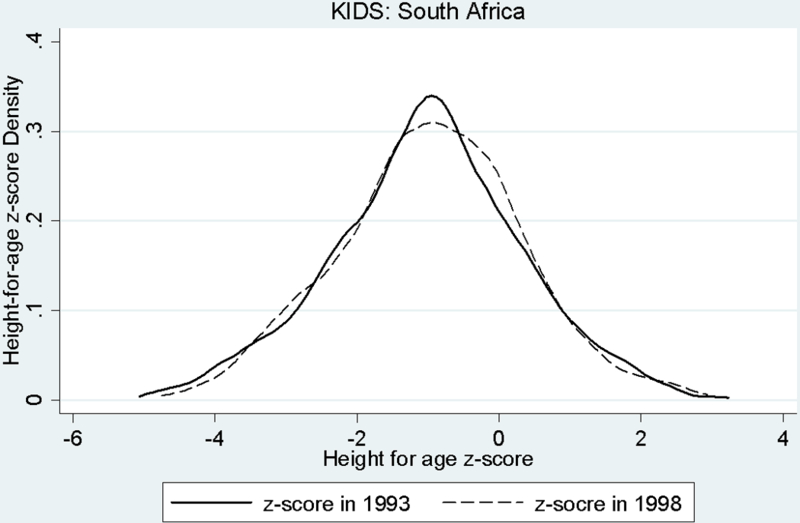
According to UN country level statistics averaging data from 1995 to 2004, the percentage of children less than five years old displaying under nutrition (height-for-age) in each country is approximately 16% (China), 25% (South Africa) and 20% (Nicaragua) (UNDP, 2004). Table 1 presents means of height-for-age z-scores and years of survey in each panel. The baseline and follow-up (1993) values of height-for-age in China are the worst (-1.23 and -1.16), closely followed by South Africa (-1.01 and -.97). Nicaraguan children start significantly better off (-0.37), however fall behind in the follow-up (-1.01), presumably because this is a younger sample and nutritional status deteriorates rapidly at younger rages and then tapers off. These distributions follow a fairly normal curve and are presented as kernel density graphs in Figures 1–3. In addition, a descriptive analysis of the percentage of movement within each sample is presented in Table 1, where the cut point is a z-score of -1.0. In each case, the percentage of children remaining either below or above -1.0 over the panel periods is greater than those moving from above to below -1.0 z-scores and vice versa. For example, among the CHNS data, approximately 45%-49% are less than -1.0 z-scores in both years and approximately 32% are above -1.0 z-scores in both years. Smaller percentages improve or regress over the panel period (10–13% and 11% respectively). In comparison to China, South Africa has a greater percentage of improvements and regressions in nutritional status, while Nicaragua shows more regressions and fewer improvements. In all cases there is enough movement to confidently examine changes in nutritional status.

Figure 1:

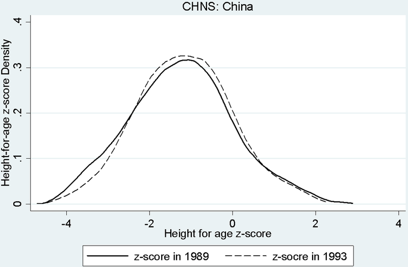
Distribution of Height-for-age z-scoresss

Figure 3:

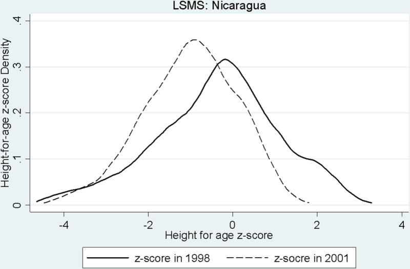
Distribution of Height-for-age z-scores

Table 2 presents the remaining core control variables measured at baseline. Children and their mothers in EMNV are on average younger than in CHNS and KIDS. Mother’s in all three samples on average are of similar stature, with the Nicaraguan mothers slightly shorter (153.2 cm) in comparison to Chinese mothers (155.5 cm) and South African mothers (157.5 cm). Height may in part be distinctive among ethnic groupings, however these account for a relatively small percentage of the sample. Approximately 11% of the South African sample is East Indian and 3% of the Nicaraguan sample is identified as Indigenous Indian. As would be expected, family size of Chinese households is the smallest (4.95 members), followed by Nicaraguan families (7.23 members) and South African families (8.71 members). The low category of mother’s education contains 12% (CHNS), 46% (KIDS) and 19% (EMNV) of the sample respectively. The percentage of households residing in urban areas varies from 9% in South Africa to 45% in Nicaragua. Finally, Figure 4 displays local linear regressions of height on lagged height for each of the 4 samples. In China the relationship appears to be the strongest, while in Nicaragua and South Africa the relationship is strongest for children between -2 and 2 z-scores but much weaker in the tails.

Figure 4:

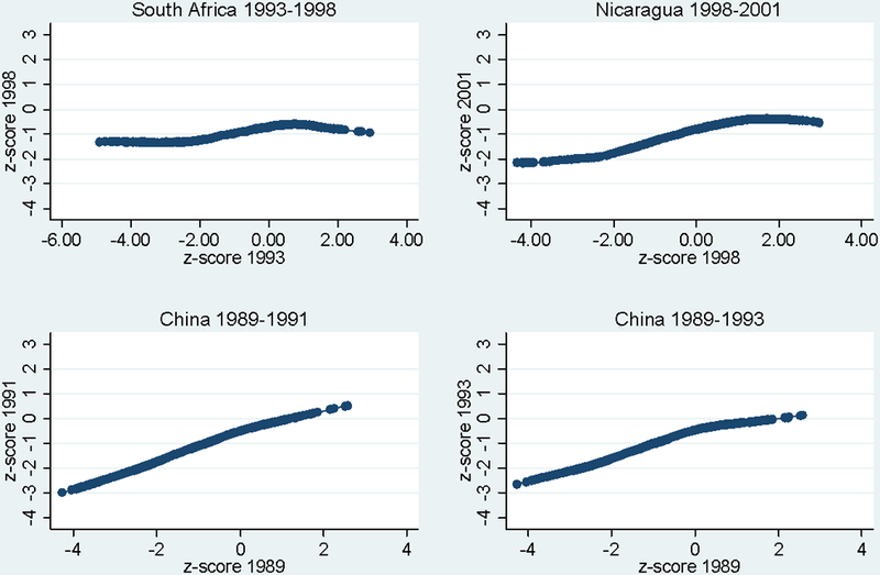
Non-Parametric Relationship of Current and Lagged Height

Notes: Figure depicts non-parametric (local linear regression) relationships between lagged (x-axis) and current (y-axis) height z-score for each of the four samples.

5B. Summary of catch-up growth effects across 3 continents

Table 3 presents a summary of the catch-up growth effects as indicated by the coefficient of lagged height z-score on current height z-score; full estimates for the control variables are provided in the appendix. A coefficient of 1 indicates complete state dependency in health or no catch-up and a coefficient of 0 indicates complete catch-up, or no persistence in health across time. For each data set the OLS coefficient of lagged z-score predicting current z-score is displayed, as well as the preferred instrumental variable coefficient which accounts for the endogeneity of lagged z-score. In all cases the OLS coefficient of lagged height-for-age is positive and significantly different from both 0 (shown) and 1 (not shown), with effect sizes highest in the 2 year panel in China (0.495) and smallest in the 5 year panel in South Africa (0.265); in the China 4 year panel the catch-up effect drops to 0.418 and is of roughly the same magnitude as in the 3 year panel in Nicaragua.

Table 3:

Summary coefficients of Lagged Height-for-age Z-scores on Current Z-score

	CHNS : China 1989–91		CHNS : China 1989–93		KIDS : South Africa		LSMS : Nicaragua
	OLS	IV	OLS	IV	OLS	IV	OLS	IV
	(1)	(2)	(3)	(4)	(5)	(6)	(7)	(8)
Coefficient	0.495	0.381	0.418	0.386	0.265	0.201	0.425	0.358
(Standard error)	(0.030)	(0.107)	(0.035)	(0.103)	(0.046)	(0.101)	(0.053)	(0.063)
t-statistic	16.50	3.56	11.94	3.75	5.76	1.99	8.02	5.68
R-squared value	0.558	0.369	0.475	0.348	0.285	0.229	0.479	0.316
Observations	1121		1121		514		497
			First stage diagnostics
F(instruments)1		14.55		14.55		9.89		1906.14
Partial R-squared (instruments only)		0.16		0.16		0.26		0.15
Overid test (all instruments) (p-value)2		0.10		0.18		0.09		0.76
Over id test (prices only)		0.13		0.36		0.05		0.81
Over id test (prices and price interactions)		0.07		0.19		0.11		0.28
Over id test (shocks only)		-		-		-		0.71
Overall R-squared	0.42			0.42		0.33		0.54

1/ Instruments are lagged prices, lagged prices interacted with mother’s education dummy and lagged wealth. For KIDS the instrument set includes rainfall shocks; in LSMS the instrument set includes rainfall and crop shocks.2/ Test statistic is distributed chi-square with degrees of freedom equal to the number of instruments less the number of endogenous variables. Standard errors for the IV models are bootstrapped. Full regression results presented in the Appendix.

The even numbered columns in Table 3 report the IV estimates that account for health related behaviors and preferences and these are all smaller than OLS, though the pattern of effect sizes is the same—the largest effects are in China (0.381 and 0.386) and Nicaragua (0.358) and the smallest effect in South Africa (0.201). The ratio of OLS to IV coefficients is between 76% and 92% in China and 84% and 76% in Nicaragua and South Africa respectively. This decrease indicates that once unobserved heterogeneity is controlled, the possibility of catch-up growth improves. Therefore, parents do not display compensating behavior, but instead engage in investment type behavior and favor innately stronger children. Alternatively, (positive) health related knowledge or preferences are positively correlated with innate health. Both of these scenarios reduce the possibility of catch-up growth, and is strongest in South Africa (where the divergence between OLS and IV is the largest), followed by the 2 year panel in China and then Nicaragua. We note that the pattern of OLS and IV estimates is also consistent with measurement error in height, so not all the difference in coefficient estimates may be due to household behaviors.

The bottom panel of Table 3 reports auxiliary statistics from the first stage regression predicting lagged height. The F-statistic for the joint significance of the instruments (prices, shocks, their interactions with maternal education and wealth) exceeds the Staiger & Stock (1997) rule of thumb of 10 except in South Africa where it is 9.89, while the partial R-squared of the instruments (Shea, 1997) only in stage 1 ranges from 15% (Nicaragua) to 26% (South Africa). We calculate the test for overidentification proposed by Sargan (1958) by regressing the residuals from the first stage regression on all the exogenous variables. The R-squared from this regression, multiplied by the number of observations, is distributed as chi-square with degrees of freedom equal to the number of overidentified instruments. The bottom of Table 3 shows the p-value for the null hypothesis that the instruments are not valid, which indicate that the full set of instruments are valid in each of the four specifications, although lagged prices by themselves may not be valid in the KIDS. Finally, we have also replicated the results in Table 3 excluding wealth from the instrument set. These results are reported in Table A6 in the Appendix, and are very similar to those reported in Table 3.

5C. Catch-up growth effects in China using alternative identification strategy

Table 4 summarizes the catch-up growth effects using the 3 equally spaced rounds (1989, 91, 93) of the CHNS and employing the Blundell & Bond GMM system estimator. The OLS estimate of the catch-up effect (column 1) is slightly larger than in the 1989–91 panel and the equivalent 2SLS estimator which uses the same exclusion restrictions as in Table 3 (reported in column 6) is only slightly smaller at 0.642. However in this sample the instruments are weak and probably irrelevant as indicated by the partial R-squared and F-statistic at the bottom of column 6. A 2SLS specification which adds the two period lagged difference in height to the instrument set performs much better (column 5) and produces a point estimate that is much lower at 0.530, or 78% of the OLS estimate.

Table 4:

Summary coefficients of Lagged Height-for-age Z-scores on Current Z-score, China 1991–1993

Estimator	OLS	Arellano-Bond	Blundell-Bond System		2SLS
	Levels	First difference	First difference		Levels	Levels	Levels
	(1)	(2)	(3)	(4)	(5)	(6)	(7)
Coefficient	0.683	0.091	0.566	0.510	0.530	0.642	0.391
(Standard error)	(0.023)	(0.110)	(0.064)	(0.085)	(0.070)	(0.083)	(0.084)
t-statistic	29.70	0.83	8.84	6.00	7.57	7.73	4.65
Instrument set
2 period lagged height	N/A	YES	YES	YES	YES1	NO	YES1
Prices, interactions and wealth	N/A	YES1	YES1	NO	YES	YES	NO
F(instruments)		1.90			11.35	2.1	108.08
Partial R-squared for stage one instruments		0.065			.296	0.04	0.130

Observations are 1130. The first difference estimator uses two period lagged height as instrument as well as lagged differences in prices and wealth. The levels equation uses the two period lagged difference in height as the instrument and lagged prices and wealth. See text for details. 1/ Measured in differences.

The GMM system estimator which uses prices, their interactions and wealth plus two period lagged height (column 3) as instruments results in a point estimate of the catch-up growth effect of 0.566, about 83% of the OLS estimate in column 1, a difference which is in line with the pattern reported in Table 3 and close to the 2SLS estimate in column 5 of Table 4. Notice that the single-equation Arellano-Bond estimator in this sample does not perform well (column 2) due to the weak instrument problem, and is precisely the motivation set forth by Blundell & Bond (1998) for the system estimator. The result in column 3, our preferred estimate, is generally consistent with those reported in Table 3 using the alternative identification strategy: unobserved heterogeneity tends to reduce catch-up growth possibilities, either because of investment type behavior by parents or because health knowledge is positively correlated with health endowment.

We are able to implement both the Arellano-Bond and the GMM system estimator because we assume that lagged height is a sufficient statistic for all previous realizations of height. Is this assumption supported by the data? If we add two-period lagged height (1989) to the specification reported in column 1 of Table 4, the coefficient of lagged height drops to 0.607 (a drop of 11 percent) and is still highly statistically significant (t=21.58) while other coefficients remain unaltered. On the other hand, the coefficient of two period lagged height is 0.128 (t=3.38), which is a 73 percent reduction from its value of 0.418 as reported in column 2 of Table 3. Thus it appears that while lagged height is not a sufficient statistic per se, an additional lag add relatively little extra information and does not affect the interpretation of other coefficients, a finding that is consistent with the education production literature (Todd & Wolpin 2007).

5D. Sub-sample estimates of catch-up growth

Table 5 presents catch-up growth effects for different sub-samples. The top panel shows results for the sub-sample of children who were at least mildly malnourished in the base year (z-score of less than -1.0). This group is of interest for two reasons. First, they are at higher risk and therefore of policy interest. Second, there is more room for improvement among this group, suggesting that the estimated coefficient on lagged z-score would be smaller among this group (the familiar regression-to-the-mean story). In two of the four estimates (South Africa and Nicaragua) the sample size for this sub-group is very small and the resulting IV point estimates are no longer statistically significant. In China where sample size continues to be large, the IV estimates are smaller than OLS, statistically different from 0, and smaller than the full sample IV estimates from Table 3, supporting the idea that catch-up growth is more likely in this group.

Table 5:

Sub Sample Summary Coefficients of Lagged Height-for-age Z-scores on Current Z-score

	CHNS : China 1989–91		CHNS : China 1989–93		KIDS : South Africa		LSMS : Nicaragua
	OLS	IV	OLS	IV	OLS	IV	OLS	IV
	(1)	(2)	(3)	(4)	(5)	(6)	(7)	(8)
Z-score<-1 at baseline
Coefficient	0.501	0.290	0.433	0.226	0.256	0.279	0.254	0.245
(Standard error)	(0.050)	(0.100)	(0.053)	(0.104)	(0.152)	(0.264)	(0.109)	(0.196)
t-statistic	10.02	2.90	8.17	2.17	1.68	1.06	2.33	1.25
R-squared value	0.437	0.306	0.479	0.345	0.279	0.301	0.428	0.409
F(instruments in first stage)		11.55		11.55		1021.10		1.10
Observations	705		705		258		149
Age<=24 months at baseline
Coefficient	0.363	0.336	0.308	0.318	0.281	0.223	0.427	0.351
(Standard error)	(0.053)	(0.084)	(0.053)	(0.069)	(0.070)	(0.182)	(0.059)	(0.141)
t-statistic	6.85	4.00	5.81	4.61	4.01	1.23	7.24	2.49
R-squared value	0.619	0.306	0.536	0.483	0.416	0.358	0.479	0.315
F(instruments in first stage)		16.09		16.09		1148.00		1.02
Observations	331		331		152		475
Age >24 months at baseline
Coefficient	0.596	0.520	0.512	0.520	0.216	0.258
(Standard error)	(0.035)	(0.12)	(0.043)	(0.128)	(0.053)	(0.119)
t-statistic	16.87	4.30	11.95	4.06	4.08	2.17
R-squared value	0.62	0.395	0.510	0.395	0.342	0.306
F(instruments in first stage)1		8.08		8.08		9700.00
Observations	790		790		362

1/ Instruments are lagged prices, lagged prices interacted with mother’s education dummy, lagged wealth and shocks. Standard errors for the IV models are bootstrapped with 1000 repetitions. Coefficients significant at 5% are in bold. The Nicaragua sample only ranges from 0–36 months at baseline so estimates for the older sub-sample are not possible.

The middle and bottom panels of Table 5 reports results based on the sub-sample of children who were less than or equal to 24 months of age and older than 24 months at baseline. In the middle panel the sample size for South Africa drops to 152 and cannot support a statistically significant t-statistic, but IV estimates are significant in the other three panels and slightly smaller than the IV estimates reported in Table 3 over the full sample. The IV results for older children, only estimable in CHNS and KIDS due to sample size, are all larger than those for younger kids and are consistent with the idea that height deficits that occur at earlier ages are more able to be reversed. These findings support a programming approach that focuses on early intervention (under age 2) of nutrition interventions.²⁴

5E. Interaction effects in the CHNS

In this section we explore the possibility that catch-up growth varies with family background and environmental factors using the CHNS. The existence of facilitators (or inhibitors) of improved growth are of policy interest because these factors could be used for targeting interventions to malnourished children or be the objective of interventions themselves. We explore interactions between lagged height and mother’s schooling, mother’s height, distance to nearest health facility, household wealth, and the sex of the child. Mother’s height and schooling have themselves been the focus of studies on the determinants of childhood malnutrition.

One possible role of maternal height is as an indicator of genetic potential. Although there is some evidence that the genetic component of the differences in children’s height is on average small in comparison to environmental influences, parental height is still a significant component of potential height (Golden, 2005). In developing countries, the idea of height potential is somewhat of a problem if the parents themselves are short because of malnutrition when they were children. This implies two very different definitions of catch-up. One is a catch-up to a standard height based on a healthy population, and the other is a catch-up to what is expected of the child, given trends of malnutrition. To catch-up by international standards or essentially correcting for generations of malnutrition may be expecting more then is plausible from any given child. However, there is evidence that suggests that not only does mother’s height indicate inherited stature, but also in part inherited disease susceptibility due to its significance on survival rates, even after controlling for other characteristics (Thomas, Strauss and Henriques, 1990). In this way, mother’s height could be thought of as a control for the ‘human capital’ of the mother or parents (Strauss and Thomas, 1995). Further, it has been suggested that the significance of parental height increases as the child ages (Cebu Study Team, 1992).

Mother’s education has been cited in numerous studies as showing strong associations with nutrition status of children (Barrera, 1990; Strauss and Thomas, 1995; Thomas, Strauss and Henriques, 1990). Education may signal knowledge in child caring, as well as a proxy indicator of earning potential, access to information and higher woman’s status. In all three data sets, mother’s education is not a significant determinant of child health, suggesting that it might be correlated with other control variables in the equation such as mother’s height and wealth score.²⁵ For example, Barrera found that estimates for mother’s education fell by between 20 and 50 percent when mother’s height is controlled for using data predicting height for age in the Philippines (Barrera, 1990). Similarly, using data from Brazil predicting child survival, Thomas, Strauss and Henriques find that the coefficient on mother’s education drops between ¼ and ⅓ in size when household income is introduced (Thomas, Strauss and Henriques, 1990).

We experimented with separate specifications that exclude mother’s height and household wealth and find that the coefficient of mother’s education is not sensitive to the exclusion of height, but is sensitive to the exclusion of wealth. Specifically, the impact of maternal education in the stage one regressions increase (in absolute terms) when wealth is excluded from the model, while in the second stage, the impact also increases in absolute value but does not become statistically significant (results available from the authors upon request).

Table 6 reports the coefficient estimate of the interaction term between lagged z-score and the indicated variable, with lagged z-score and its interaction treated as endogenous and reported t-statistics based on bootstrapped standard errors. The interpretation of the sign of the interaction term depends on the way the variable is measured. If higher values of the variable are thought to be positively correlated with height (e.g. wealth and maternal height), then a positive interaction indicates a factor which exacerbates earlier malnutrition while a negative one indicates a factor which mitigates earlier malnutrition. However if the variable is measured such that lower values are thought to be positively associated with better nutrition (such as distance to health facility, and mother’s education since our indicator is for low maternal education) than the opposite is the case: a negative coefficient exacerbates and a positive one mitigates. Since the catch-up growth hypothesis is supported when the impact of lagged z-score is closer to zero, factors that mitigate improve the chance of catch-up growth. Results in Table 6 do not show any statistically significant interactions except for maternal education, which appears to mitigate the impact of earlier malnutrition.

Table 6:

Coefficient Estimates of Lagged Height Interacted with Household/Environmental Factors

	CHNS: China 1989–91		CHNS : China 1989–93
Interaction of lagged height z-score with:	Interaction	Lagged Height	Interaction	Lagged Height
Maternal education	−0.268	0.412	−0.040	0.391
standard error	0.125	0.059	0.114	0.066
(t-statistic)	(2.14)	(6.98)	(0.35)	(5.92)
Maternal height	−0.001	0.537	0.001	0.241
standard error	0.006	0.928	0.008	1.160
(t-statistic)	(0.17)	(0.58)	(0.13)	(0.21)
Household wealth index	−0.005	0.381	0.012	0.385
standard error	0.047	0.061	0.047	0.064
(t-statistic)	(0.11)	(6.25)	(0.26)	(6.02)
Distance to nearest health facility	0.027	0.367	0.046	0.367
standard error	0.016	0.062	0.039	0.066
(t-statistic)	(1.69)	(5.92)	(1.18)	(5.56)
Male	0.052	0.355	0.097	0.335
standard error	0.069	0.072	0.071	0.077
(t-statistic)	(0.75)	(4.93)	(1.37)	(4.35)

Each row represents a separate regression. Lagged height and its interaction treated as endogenous, standard errors bootstrapped with 1000 repetitions. Coefficients in bold are significant at 5%.

6. Discussion and conclusions

The possible existence of catch-up growth has attracted the attention of economists and public health researchers due to the growing evidence that early childhood malnutrition is associated with a range of adverse outcomes at later life stages. Researchers have approached the question in different ways, using a variety of sample designs (lag lengths and age groups), statistical techniques and measures of nutritional status. Three key points stand-out from our review of the literature: 1) the endogeneity of lagged health on current or future health is not fully accounted for in many of the studies; 2) the preferred measure of nutritional status is in z-scores and not actual height in centimeters or ranges as is common in some of the literature; 3) there is no consensus on the possibility of catch-up growth based on population samples, but this is not surprising given the variation in statistical techniques, measures and sample design.

We contribute to the catch-up growth debate by presenting results from three widely varying population based samples using identical statistical techniques, controlling for endogeneity of lagged health in several different ways, and measuring height in z-scores. Our estimates of the association between lagged and current z-score based on OLS range from 0.265 to 0.683 for these three different populations, indicating that while previous health does not track future health perfectly, there is still significant persistence in health status for young children. These estimates do not account for household health-related behavior. When such behavior is accounted for, point estimates are reduced to the 0.201–0.566 range. While this drop implies a greater possibility of catch-up growth, the point estimates are still significantly different from zero, indicating some persistence in health status. This basic result is robust to our identification strategy and to height measured in centimeters.

The relative magnitudes of the OLS and IV point estimates indicate that household behavioral decisions about children’s health reduce the possibility of catch-up growth. This is consistent with several alternative explanations of household behavior: 1) that households pursue an investment or wealth maximizing strategy and invest more in children with better innate health endowment, or; 2) that (positive) household knowledge and caring practices are positively associated with health endowments and thus exacerbate initial differences in health. The difference between the OLS and IV estimates of catch-up growth represents the behavioral component of the catch-up phenomenon, and thus provides a rough indication of the extent to which child growth can be influenced by public policy. To better understand the potential magnitudes we simulate the distribution of z-scores in the later period based on the IV and OLS point estimates reported in Table 3, holding other variables at the means and using other coefficients from the preferred IV model. Table 7 shows the potential influence on mean height z-score if public policy could reduce the negative behavioral effect estimated in this paper. In China the scope for public policy seems to be limited as the IV and OLS predictions of mean height at follow-up are very similar. On the other hand, the differences in South Africa (0.46 standard deviations) and Nicaragua (0.51 standard deviations) are quite substantial, and as noted in the introduction, these improvements can have substantial implications for later school attainment, learning and ultimately economic productivity. Based on the results in this paper, we conclude that catch-up growth in linear height among children in developing countries is possible, especially when the child is less than 24 months of age.

Table 7:

Simulations of mean follow-up Z-scores

	China 1991		China 1993		South Africa		Nicaragua
Lagged z-score coefficient estimated by :	Mean	SD	Mean	SD	Mean	SD	Mean	SD
OLS	−1.564	(0.63)	−1.152	(0.67)	−1.592	(0.61)	−1.527	(0.85)
Instrumental Variables	−1.426	(0.48)	−1.136	(0.49)	−1.125	(0.26)	−1.013	(0.52)

Means based on predicted distribution of height z-score in the follow-up period using the regression models in Table 3, holding all other variables at the means, and varying the coefficient of z-score as indicated in the first column.

Figure 2:

Distribution of Height-for-age z-scores

Appendix

Table A1:

Variables used in Principal Component Analysis of Wealth Score

	CHNS : China	KIDS : South Africa	LSMS : Nicaragua
(1)	Television (=1)	Flush Toilet (=1)	Number of rooms
(2)	Piped water (=1)	Piped water (=1)	Electricity (=1)
(3)	Radio (=1)	Refrigerator (=1)	Television (=1)
(4)	Interior toilet (=1)	Telephone (=1)	Stove (=1)
(5)	Electricity (=1)	Electricity (=1)	Electric fan (=1)
(6)	VCR (=1)	Radio (=1)	Refrigerator (=1)
(7)	Bicycle (=1)	Bicycle (=1)	Iron (=1)
(8)	Scooter/motorbike (=1)		Piped water (=1)
(9)	Car (=1)		Non-dirt floor (=1)
(10)	Sheep (=1)		VCR (=1)
(11)	Chicken (=1)		Sewing machine (=1)
(12)	Horse (=1)		Flush toilet (=1)
(13)	Pig (=1)		Bicycle (=1)
(14)			Car (=1)
(15)			Toaster (=1)
(16)			Oven (=1)
(17)			Scooter/motorbike (=1)
(18)			Washing machine (=1)

^*Principle components are listed in order of their contribution to the score in the baseline; higher contributing variables are listed first.

Table A2:

Correlation coefficients of per capita income and wealth index

	China		South Africa	Nicaragua
	1989–91	1989–93
Wealth index across years	0.80	0.76	0.88	0.86
Income across years	0.39	0.35	0.75	0.63
Contemporaneous wealth and income (baseline)	0.40	0.40	0.55	0.41
Contemporaneous wealth and income (follow-up)	0.40	0.38	0.53	0.31

In South Africa pc expenditure is used instead of pc income.

Table A3:

Second Stage Height-for-age estimates for KwaZulu-Natal Income Dynamics Survey

	(1)		(2)
	OLS		IV
Variables	Coefficient	SE	Coefficient	SE
Lagged Height for age z-score	0.265	(0.05)	0.201	(0.09)
Child Level Variables:
Age (years)	−0.100	(0.03)	−0.094	(0.04)
Male (=1)	0.081	(0.10)	0.081	(0.11)
East Indian ( =1)	3.494	(0.52)	3.567	(0.54)
Mother’s age (in years)	0.066	(0.07)	0.055	(0.07)
Mother’s age squared (in years X100)	−0.091	(0.00)	−0.077	(0.00)
Mother’s Education <= primary (=1)	0.153	(0.15)	0.142	(0.15)
Missing information on mother (=1)	−0.129	(0.20)	−0.109	(0.22)
Mother’s height (in cm)	0.027	(0.01)	0.027	(0.01)
Household Level Variables:
Household size	0.004	(0.02)	0.002	(0.02)
Wealth score	−0.007	(0.14)	−0.006	(0.16)
Community Level Variables:
Urban	−0.309	(0.56)	−0.258	(0.63)
Metro	−0.382	(0.61)	−0.387	(0.66)
R-squared	0.291		0.229

Observations are 514. Community level prices of 32 foods and basic items, a constant term and 29 magisterial district dummy variables included but not reported.

Table A4:

Second Stage Height-for-age estimates for Nicaraguan EMNV

	OLS		IV
Variable	Coefficient	SE	Coefficient	SE
Child Level Variables:
Lagged Height for age z-score	0.425	(0.05)	0.358	(0.07)
Male (=1)	−0.115	(0.06)	−0.126	(0.08)
Age 7–12 months	0.583	(0.12)	0.536	(0.15)
Age 13–36 months	0.924	(0.10)	0.816	(0.13)
Mother’s age (in years)	0.014	(0.04)	0.022	(0.05)
Mother’s age squared (in years X100)	−0.022	(0.00)	−0.036	(0.00)
Mother’s height (in cm)	0.009	(0.01)	0.010	(0.01)
Indigenous Indian (=1)	−0.514	(0.09)	−0.582	(0.10)
Missing information on mother (=1)	0.096	(0.23)	0.064	(0.33)
Mother Illiterate (=1)	0.028	(0.10)	0.005	(0.10)
Household Level Variables:
Household size	−0.018	(0.014)	−0.024	(0.017)
Wealth score	0.259	(0.07)	0.279	(0.07)
Log of distance to clinic (in min)	0.015	(0.03)	0.039	(0.04)
Urban (=1)	−0.345	(0.17)	0.272	(0.16)
Household suffered drought	0.081	(0.09)	0.165	(0.14)
Household experienced crop loss due to pests	0.060	(0.08)	−0.017	(0.11)
Observations	497		497
R-squared	0.479		0.316

Estimates include a constant, prices of 22 foods and other items and 17 regional dummy variables for departments which are not reported here.

Table A5:

Second Stage Height-for-age Estimates for China Health and Nutrition Survey

	(1) OLS		(2) IV		(3) OLS		(4) IV
Variable	Coefficient	SE	Coefficient	SE	Coefficient	SE	Coefficient	SE
Child Level Variables:
Lagged Height for age z-score	0.495	(0.03)	0.381	(0.11)	0.418	(0.03)	0.386	(0.10)
Male (=1)	0.048	(0.05)	0.060	(0.06)	0.073	(0.05)	0.071	(0.05)
age 7–12 months	0.298	(0.14)	0.222	(0.15)	0.485	(0.11)	0.441	(0.13)
age 13–24 months	0.493	(0.13)	0.316	(0.13)	0.398	(0.11)	0.318	(0.11)
age 25–36 months	0.347	(0.12)	0.255	(0.13)	0.237	(0.12)	0.244	(0.13)
age 37–48 months	0.340	(0.14)	0.223	(0.15)	0.161	(0.11)	0.127	(0.14)
age 49–60 months	0.351	(0.14)	0.218	(0.15)	0.249	(0.12)	0.218	(0.14)
age > 60 months	0.202	(0.13)	0.007	(0.15)	0.402	(0.12)	0.299	(0.14)
Mother’s age (in years)	−0.002	(0.01)	0.000	(0.01)	0.003	(0.01)	0.004	(0.01)
Mother’s height (in cm)	0.039	(0.01)	0.044	(0.01)	0.032	(0.01)	0.033	(0.01)
mother completed primary school	−0.035	(0.10)	−0.010	(0.12)	0.038	(0.07)	0.046	(0.09)
mother completed secondary	−0.144	(0.11)	−0.111	(0.13)	−0.019	(0.08)	−0.012	(0.10)
Household Level Variables:
Wealth score	0.122	(0.04)	0.148	(0.05)	0.130	(0.05)	0.138	(0.05)
Household size	0.003	(0.02)	0.001	(0.02)	0.002	(0.02)	0.004	(0.02)
Community Level Variables:
Log of distance to clinic (in min)	0.008	(0.01)	0.010	(0.01)	−0.031	(0.03)	−0.031	(0.03)
Main access road is paved	0.203	(0.07)	0.212	(0.07)	0.168	(0.07)	0.178	(0.07)
population/100	0.000	(0.11)	0.000	(0.09)	0.000	(0.00)	0.000	(0.00)
Year	1991				1993
R-squared	0.558		0.369		0.475		0.348

Regressions include constant, 12 prices, community wage rate, and 47 county dummy variables which are not reported here.

Table A6:

Summary coefficients of Lagged Height-for-age Z-scores on Current Z-score Excluding Wealth from Instrument Set

	CHNS : China 1989–91		CHNS : China 1989–93		KIDS : South Africa		LSMS : Nicaragua
	OLS	IV	OLS	IV	OLS	IV	OLS	IV
	(1)	(2)	(3)	(4)	(5)	(6)	(7)	(8)
Coefficient	0.495	0.375	0.418	0.378	0.265	0.195	0.425	0.383
(Standard error)	(0.030)	(0.071)	(0.035)	(0.068)	(0.046)	(0.097)	(0.053)	(0.063)
t-statistic	16.50	5.31	11.94	5.57	5.76	2.01	8.02	6.05
Observations	1121		1121		514		497
			First stage diagnostics
F(instruments)1		21.39		21.39		9.76		1841.75
Partial R-squared (instruments only)		0.12		0.12		0.25		0.14
Overall R-squared		0.42		0.42		0.33		0.51

1/ Instruments are lagged prices and lagged prices interacted with mother’s education dummy. For KIDS the instrument set includes rainfall shocks; in LSMS the instrument set includes rainfall and crop shocks. Standard errors for the IV models are bootstrapped.

Table A7:

Prices used in stage one regressions

China	South Africa	Nicaragua
Rice	Maize	Tortilla
Wheat	Mealie meal	Red beans
Noodles	Rice	Corn
Sugar	Bread	Bread
Eggs	Flour	Sugar
Cabbage	Cereal	Vinegar
Vegetable	Pulses	Salt
Beef	Potato	Beef
Powdered milk	Tomato	Pork
Coal	Sweet potato	Chicken
Unskilled wage	Vegetable Oil	Milk
Construction wage	Butter	Cheese
Rice (SS)	Cheese	Eggs
Wheat (SS)	Milk	Tomato
Noodles (SS)	Formula	Onion
Cabbage (SS)	Sugar	Potato
Vegetable (SS)	Meat	Plantain
Beef (SS)	Chicken	Oranges
Powdered milk (SS)	Eggs	Coal
	Fish	Cigarettes
	Tin fish	Soap
	Pumpkin	Toilet paper
	Banana
	Apples
	Soft drinks
	Cigarettes
	Washing powder
	Toilet paper
	Soap
	Toothpaste
	Paraffin
	Charcoal

SS indicates State Store. Other prices in China are from Free Market Stores.

References

- Adair LS. Filipino Children Exhibit Catch-up Growth from Age 2 to 12 years. Community and International Nutrition 1999; 129; 1140–1148. [DOI] [PubMed] [Google Scholar]
- Alderman H, Behrman JR, Levy V, Menon R. Child Health and School Enrollment: A Longitudinal Analysis. The Journal of Human Resources 2001; 36(1); 185–205. [Google Scholar]
- Alderman H, Hoddinott J, Kinsey B. Long-Term Consequences of Early Childhood Malnutrition. Oxford Economic Papers 2006; 58:450–474. [Google Scholar]
- Alderman H, Hoogeveen H & Rossi M Preschool Nutrition and Subsequent Schooling Attainment: Longitudinal Evidence from Tanzania. Economic Development & Cultural Change 2009; 57(2):239–260. [Google Scholar]
- Arellano M, & Bond S (1991). Some Tests of Specification for panel Data-Monte Carlo Evidence and an Application to Employment Equations. Review of Economic Studies, 58(2), 277–297. [Google Scholar]
- Arellano M, & Bover O Another look at the Instrumental Variable Estimation of Error-Components Models. Journal of Econometrics 1995; 68: 29–51. [Google Scholar]
- Barrera A The role of maternal schooling and its interaction with public health programs in child health production. Journal of Development Economics 1990; 32; 69–91. [Google Scholar]
- Bhargava A Identification and Panel Data Models with Endogenous Regressors. Review of Economic Studies 1991; 58: 129–140. [Google Scholar]
- Boersma B, Wit JM. Catch-up Growth, Endocrine Reviews 1997; 18(5); 646–661. [DOI] [PubMed] [Google Scholar]
- Bollen KA, Guilkey DK, Mroz TA. Binary Outcomes and Endogenous Explanatory Variables: Test and Solutions with an Application to the Demand for Contraceptive Use in Tunisia. Demography 1995; 32(1); 111–131. [PubMed] [Google Scholar]
- Blundell R, & Bond S (1998). Initial conditions and moment restrictions in dynamic panel data models. Journal of Econometrics, 87(1), 115–143. [Google Scholar]
- Cameron AC, Trivedi PK. Microeconometrics 2005; Cambridge University Press. [Google Scholar]
- Cameron N Physical growth in a transitional economy: the aftermath of SA apartheid. Economics and Human Biology 2003; 1; 29–42. [DOI] [PubMed] [Google Scholar]
- Cameron N, Preece MA, Cole TJ. Catch-up Growth or Regression to the Mean? Recovery from Stunting Revisited. American Journal of Human Biology 2005; 17; 412–417. [DOI] [PubMed] [Google Scholar]
- Carolina Population Center. The China Health and Nutrition Survey. The University of North Carolina, Chapel Hill, NC: 2005; Available at http://www.cpc.unc.edu/projects/china/. [Google Scholar]
- Carter MR, Maluccio JA. Social Capital and Coping with Economic Shocks: An Analysis of Stunting of South African Children. World Development 2003; 31(7); 1147–1163. [Google Scholar]
- Carter MR, Haddad L, May J, Maluccio JA. KwaZulu-Natal Income Dynamics Study (KIDS) 1993–1998, Overview and Description of Data Files. International Food Policy Research Institute, University of Natal-Durban and University of Wisconsin-Madison; 2003. [Google Scholar]
- Cebu Study Team (Akin J, Guilkey D, Popkin B). A child health production function estimated from longitudinal data. Journal of Development Economics 1992; 38; 323–351. [PubMed] [Google Scholar]
- Checkley W, Epstein LD, Gilman RH, Black RE, Cabrera L, Sterling CR. Effects of Cryptosporidium parvum Infection in Peruvian Children: Growth Faltering and Subsequent Catch-up Growth. American Journal of Epidemiology 1998; 148(9); 497–506. [DOI] [PubMed] [Google Scholar]
- Fedorov L, Sahn DE. Socioeconomic Determinants of Child’s Health in Russia. Economic Development and Cultural Change 2005; 53; 479–500. [Google Scholar]
- Fitzgerald J, Gottschalk P, Moffit R, (1998), “An analysis of sample attrition in panel data”, in Journal of Human Resources, 33(2), p. 251–299. [Google Scholar]
- Foster AD. Prices, Credit Markets and Child Growth in Low-Income Rural Areas. The Economic Journal 1995; 105(430); 551–570. [Google Scholar]
- Gafni RI, Baron J. Catch-up growth: possible mechanisms. Pediatric Nephrology 2000; 14; 616–619. [DOI] [PubMed] [Google Scholar]
- Glewwe P, King EM. The Impact of Early Childhood Nutritional Status on Cognitive Development: Does the Timing of Malnutrition Matter? World Bank Economic Review 2001; 15(1); 81–113. [Google Scholar]
- Glewwe P, Jacoby HG, King EM. Early childhood nutrition and academic achievement: a longitudinal analysis. The Journal of Public Economics 2001; 81; 345–368. [Google Scholar]
- Golden MHN. Is complete catch-up growth possible for stunted children? European Journal of Clinical Nutrition 1994; 48(Suppl. 1); S58–S71. [PubMed] [Google Scholar]
- Grantham-McGregor S, Cheung YB, Cueto S, Glewwe P, Richter L, & Strupp B (2007). Developmental potential in the first 5 years for children in developing countries. Lancet, 369(9555), 60–70. [DOI] [PMC free article] [PubMed] [Google Scholar]
- Handa S, Peterman A. Child Health and School Enrollment: A Replication. Journal of Human Resources 2007; 42(4); 863–880. [Google Scholar]
- Hoddinott J, Kinsey B. Child growth in the time of drought. Oxford Bulletin of Economics and Statistics 2001; 63(4); 409–436. [Google Scholar]
- International Food Policy Research Institute (IFPRI), University of Natal-Durban and the University of Wisconsin-Madison. KwaZulu-Natal Income Dynamics Study (KIDS) 1993–1998: Overview and Description of Data Files, Release Version 3. 2003.
- Knops NBB, Kommer CAS, Brand R, Hille ETM, den Ouden AL, Wit JM, Verloove-Vanhorick SP. Catch-up growth up to ten years of age in children born very preterm or with very low birthweight. BMC Pediatrics 2005; 5(26). [DOI] [PMC free article] [PubMed] [Google Scholar]
- Li H, Stein AD, Barnhart HX, Ramakrishnan U, Martorell R. Associations between prenatal and postnatal growth and adult body size and composition. The American Journal of Clinical Nutrition 2003; 77: 1498–1505. [DOI] [PubMed] [Google Scholar]
- Liu H, Mroz T, & Adair L Parental Compensatory Behaviors and Early Child Health Outcomes in Cebu, Philippines. Journal of Development Economics 2009; 90: 209–230. [DOI] [PMC free article] [PubMed] [Google Scholar]
- Martorell R 1997. Undernutrition during pregnancy and early childhood: consequences for cognitive and behavioral development In: Young ME, (Ed) Early child development: investing in our children’s future. Amsterdam and New York: Elsevier Science BV: 37–83. [Google Scholar]
- Martorell R The nature of child malnutrition and its long-term implications. In special issue on Public Nutrition: The Food and Nutrition Bulletin 1999; 20(3); 288– 292. [Google Scholar]
- Martorell R, Rivera J, Kaplowitz H 1990. Consequences of Stunting in Early Childhood for Adult Body Size in Rural Guatemala, in International Committee of Pediatricians (Eds), Annales Nestle Long Term Consequences of Nutrition in Infancy and Childhood 48. Vevey, Switzerland Nestle Ltd: 85–92. [Google Scholar]
- Martorell R, Khan LK, Schroeder DG. Reversibility of stunting—epidemiologic findings in children from developing countries. European Journal of Clinical Nutrition 1994; 48; S45–57. [PubMed] [Google Scholar]
- May J, Carter MR, Haddad L, Maluccio J. KwaZulu-Natal Income Dynamics Study (KIDS) 1993–1998: A longitudinal household data set for South African policy analysis. Development Southern Africa 2000; 17(4); 567–581. [Google Scholar]
- Monyeki KD, Cameron N, Getz B. Growth and Nutritional Status of Rural South African Children 3–10 years old: Ellisras Growth Study. American Journal of Human Biology 2000; 12(1); 42–49. [DOI] [PubMed] [Google Scholar]
- Mosley WH, Chen, LC 1984. An Analytical Framework for the Study of Child Survival in Developing Countries, In Child Survival: Strategies for Research (Eds) Mosley WH, Chen LC. Supplement to Population and Development Review 10: 25–48. [Google Scholar]
- Ong KKL, Ahmed ML, Emmett PM, Preece MA, Dunger DB The ALSPAC Study Team. Association between postnatal catch-up growth and obesity in childhood: prospective cohort study. British Medical Journal 2000; 320; 967–971. [DOI] [PMC free article] [PubMed] [Google Scholar]
- Osberg L, Shao X, & Xu K. The Growth of Poor Children in China 1991–2000: Why Food Subsidies May Matter. Health Economics 2009; 18: S89–S108. [DOI] [PubMed] [Google Scholar]
- Paxson C, & Case A Stature and Status: Height, Ability and Labor Market Outcomes. Journal of Political Economy 2008; 116(3): 499–532. [DOI] [PMC free article] [PubMed] [Google Scholar]
- Pelletier DL, Frongillo EA, Habicht JP. Epidemiologic evidence for a potentiating effect of malnutrition on child mortality. American Journal of Public Health 1993; 83(8); 1130–1133. [DOI] [PMC free article] [PubMed] [Google Scholar]
- Popkin BM, Richards MK, Montiero CA. Stunting is associated with overweight in children of four nations that are undergoing the nutrition transition. Journal of Nutrition 1996; 126(12): 3009–3016. [DOI] [PubMed] [Google Scholar]
- Prader A, Tanner JM, von Harnack G. Catch-up growth following illness or Starvation. An example of developmental canalization in man. Journal of Pediatrics 1963; 62; 646–659. [DOI] [PubMed] [Google Scholar]
- Saleemi MA, Ashraf RN, Mellander L, Zaman S. Determinants of stunting at 6, 12, 24 and 60 months and postnatal linear growth in Pakistani children. Acta Paediatrica. 2001; 90(11): 1304–1308. [DOI] [PubMed] [Google Scholar]
- Sargan John D. (1958) "The Estimation of Economic Relationships Using Instrumental Variables", Econometrica 26: 393–415 [Google Scholar]
- Shea J (1997). Instrument relevance in multivariate linear models: A simple measure. Review of Economics & Statistics, 79(2), 348–352. [Google Scholar]
- Shrimpton R, Victora CG, de Onis M, Lima RC, Blossner M, & Clugston G (2001). Worldwide timing of growth faltering: implications for nutritional interventions. Pediatrics, 107(5), E75–84. [DOI] [PubMed] [Google Scholar]
- Staiger D, & Stock JH (1997). Instrumental Variables Regression with Weak Instruments. Econometrica, 65(3), 557–586. [Google Scholar]
- Smith LC, Haddad L. Overcoming Child Malnutrition in Developing Countries: Past Achievements and Future Choices A 2020 Vision for Food, Agriculture and the Environment 2000. IFPRI, brief No. 64:1–2. [Google Scholar]
- Stampini M, Davis B. Discerning Transient from Chronic Poverty in Nicaragua: Measurement with a Two Period Panel Data Set. ESA Working Paper No. 03–03 2003. Agriculture and Economic Development Analysis Division: The Food and Agriculture Organization of the UN. [Google Scholar]
- Steckel RH (1995). Stature and the Standard of Living. Journal of Economic Literature, 33(4), 1903–1940. [Google Scholar]
- Strauss J, Thomas D 1995. Human Resources: Empirical Modeling of Household and Family decisions In: Handbook of Development Economics, 1995; 3A, (Ed) Behrman J, Srinivasan TN. Amsterdam: North-Holland. [Google Scholar]
- Strauss J & Thomas DT(2007). “Health Over the Life Course,” Ch. 54 in Schultz TP & Strauss John, (Ed.). Handbook of Development Economics (Vol. 4) Amsterdam: North-Holland. [Google Scholar]
- Strauss J, & Thomas DT (1998). Health, Nutrition, and Economic Development. Journal of Economic Literature, 36(2), 766–817. [Google Scholar]
- Lancet The. Special issue on Early Childhood Development 2007; 369 (Jan. 6); 69. [Google Scholar]
- Thomas DJ, Strauss J, Henriques HM. How does mother’s education affect child height? Journal of Human Resources 1991; 26(2); 183–211. [Google Scholar]
- Todd P and Wolpin K (2007). "The Production of Cognitive Achievement in Children: Home, School, and Racial Test Score Gaps." Journal of Human Capital 1(1): 91–136 [Google Scholar]
- UNDP (United Nations). Human Development Report, 2004: Cultural Liberty in Today’s Diverse World. Human Development Indicators; 2004. [Google Scholar]
- UNICEF (United Nations Children’s Fund). Progress for Children: A report card on nutrition: Number 4 UNICEF, New York: 2006. [Google Scholar]
- Vella V, Tomkins A, Borghesi A, Milgliori GB, Oryem VY. Determinants of Stunting and Recovery from Stunting in Northwest Uganda. International Journal of Epidemiology 1994; 23(4); 782–786. [DOI] [PubMed] [Google Scholar]
- Victoria CG, Barros FC. Commentary: The catch-up dilemma—relevance of Leitch’s ‘low-high’ pig to child growth in developing countries. International Journal of Epidemiology 2001; 30; 217–220. [DOI] [PubMed] [Google Scholar]
- Wilson PN, Osbourn DF. Compensatory growth after under-nutrition in mammals and birds. Biological Reviews 1960; 35; 324–363. [DOI] [PubMed] [Google Scholar]
- WHO (World Health Organization). The World Health Report 2005: Make every mother and child count 2005; WHO, Geneva. [Google Scholar]
- WHO (World Health Organization). Physical Status: The use and interpretation of Anthropometry. WHO Technical Report Series; 1995; No. 854; Geneva. [PubMed] [Google Scholar]
- World Bank, Repositioning Nutrition as Central to Development, Washington DC: 2006. [Google Scholar]
- World Bank. Poverty and Human Resources Development Research Group 2002. Nicaragua Living Standards Measurement Study Survey, Washington DC. [Google Scholar]