A novel approach of NPSO on dynamic weighted NHPP model for software reliability analysis with additional fault introduction parameter

Abstract

This paper presents software fault detection, which is dependent upon the effectiveness of the testing and debugging team. A more skilled testing team can achieve higher rates of debugging success, and thereby removing a larger fraction of faults identified without introducing additional faults. A complex software is often subject to two or more stages of testing that exhibits distinct rates of fault discovery. This paper proposes a two-stage Enhanced neighborhood-based particle swarm optimization (NPSO) technique with the assimilation of the three conventional non homogeneous Poisson process (NHPP) based growth models of software reliability by introducing an additional fault introduction parameter. The proposed neuro and swarm recurrent neural network model is compared with similar models, to demonstrate that in some cases the additional fault introduction parameter is appropriate. Both the theoretical and predictive measures of goodness of fit are used for demonstration using data sets through NPSO.

1. Introduction

The ever-increasing demand of computer software plays a crucial role not only in scientific and industrial enterprise, but also in our daily life. The development of reliable software products with increasing size and complexity is a very strenuous and challenging task. We require a software that must be reliable ([1], [2], [3]). The IEEE [4] defines software reliability as: “The probability that software will not cause a system failure for a specified time under specified conditions”. Reliability is certainly the prime factor to be claimed for study of any discipline of engineering as it quantitatively measures quality, and the quantity can be properly engineered ([5], [6], [7]). Software reliability is a propensity to improve and it can be treated as a growth factor during the testing process ([4], [5], [7], [9], [10], [12], [13], [14]).

There is no universal model for software reliability prediction, rather every model has its own special functionality for better reliability prediction. The NHPP S-shaped model is shown to be very useful in fitting software failure data. The testing process of software reliability model considers fault detection ([8], [15], [16]) and fault isolation. In general, NHPP growth model with imperfect debugging ([7], [17], [18]) is one of the best kind of analytical framework, which is used to approximate mean value function (MVF) of exponential growth, considering that the failure occurrence is up to a certain point of time. During the past three decades, the NHPP growth curve model has been applied in different researches such as: evaluation of agriculture, exchange of transportation systems, development of discoveries, transformation of aircraft industry, the evolution of telecommunication systems and statistical modeling [19]. Therefore, it is difficult to find an area of system evolution, where NHPP growth curves analysis has yet not been applied upon. The NHPP growth modeling is very useful for interpretation with the progress of testing and debugging [13]. Several researchers have investigated NHPP based SRGMs in software reliability engineering ([5], [11], [10], [20], [21]). A pioneer attempt was made by Goel and Okumoto [22] in developing NHPP exponential curve for presenting the software failure phenomenon ([58], [59]). Jinyong [18] presented a nonlinear, NHPP imperfect software debugging model with fault introduction. The Artificial Neural Network (ANN) model is as an optimization tool to solve non-linear continuous function with arbitrary accuracy. Karunanithi et al. [23] presented that neural network models have more accurate endpoint prediction compared to some analytic models. Khoshgoftaar and Szabo [24] used ANN for prediction of number of faults occur at testing phase. Tian and Noore [25] explored an evolutionary ANN for software cumulative failure time prediction based on multiple-delayed-input and single-output architecture. Zheng [26] described an ensemble of ANNs for prediction of software reliability. Su and Huang [27] proposed dynamic weighted combinational model (DWCM) based on ANN [60], [61] for prediction of software reliability. Kapur et al. ([28], [29]) presented generalized dynamic integrated model using ANN to incorporate learning phenomenon with complexity of faults. Qiuying [30] proposed a testing-coverage software reliability model that not only considers the imperfect debugging, but also the uncertainty of operating environments. Chuang et al. [31] presented dynamically weighted ensemble-based prediction system for adoptively modeling. Discrete SRGMs are needed for modeling discrete software failure data for better goodness of fit performance. Pooja and Mahapatra [32] proposed DWCM approach using ANN 2-stage architecture by combining the imperfect debugging models [62].

Many attempts have been introduced in literature to address the Neural Network (NN) ([33], [34], [35], [36], [37]) and PSO ([38], [39], [40], [41], [42], [43]) which offer promising approaches to software reliability estimation and prediction in NHPP modeling ([44], [21]). In this paper, in order to improve the ability of neural network to get away from confined on local optimum, the proposed PSO algorithm is applied to update the network based on neighborhood PSO.

PSO is a simple and efficient algorithm to solve non-linear optimization problem as it controls fewer parameters, and has better convergence performance compared to other soft computing paradigms [45]. Further in this field, Riccardo and James [39] defined additional variation in the algorithm. Bai [46] reviewed advantages and the shortcomings of PSO techniques. Eberhart and Shi [47] proposed the best approach of use of the constriction factor under maximum velocity constraint on each dimension. Li et al. [12] proposed a hierarchical mixture of software reliability models using an expectation–maximizing algorithm to estimate the prediction parameters. An adaptive inertia weight investigated by Xu [37]. Nasir et al. [48] presented dynamic neighborhood learning PSO. Wang et al. [40] proposed good balance between global search and local search by suggesting a trade-off between exploration and exploitation abilities. Sun et al. [41] presented constrained optimization problems using PSO algorithm. Mousa et al. [49] solved multi-objective optimization problem in local search based on hybrid PSO algorithm. Cong [50] explored quantum PSO algorithm, to optimize parameter of NHPP based SRGM testing effort function. Viet-Hung [51] introduced a robust optimization method based on differential evolution algorithm [52]. Huang [53] described particle-base simplified swarm optimization algorithm while considering updating mechanism to increase software reliability. Wang [54] proposed optimized method to improve NHPP model. In this paper, we propose a two-stage Enhanced NPSO technique based on the assimilation of three well known NHPP based software reliability growth models for software reliability prediction.

Imperfect debugging models can characterize the quality of software fault removal in addition to the rate of faults discovered. This paper approaches recurrent NN architecture on NHPP based software reliability growth model (SRGM), incorporating imperfect debugging phenomenon. We have modified fault introduction rate by taking into consideration the efficiency of testing team skill during software development. The paper focuses to identify the superiority of the use of the existing model proficiently, rather than developing a generalized and potentially complicated model. Consequently, a DWCM is proposed, which considers the large learning capability factor during the testing and debugging process. The novelty of this proposed work is to give more attention on fault introduction rate in imperfect debugging.

The rest of the paper is rolled out in the following way: Section 2 describes the proposed model derivation, and presents the applied methodology in detail. Section 2.2 introduces the proposed PSO with implementation of modified algorithm using neural networks. In Section 2.5, we define model validation and failure data description, along with the fitness function and predictive validity criteria. Section 2.8 gives the experimental evaluation carried out through the experiments, result, and summary. Finally, Section 3 concludes the paper based up on the outcomes of the analysis and prediction.

2. Main text

Due to lack of knowledge regarding the very particular debugging process for the specific software, the introduction rate of fault is higher and the count of errors increase at the starting of the testing stage. Based upon this practical idea, we have chosen software reliability models based on the fault introduction rate α. The proposed model can be applied on the software reliability model having higher fault introduction rate at the starting compared to the end of testing phase. Error detection rate, error content, and the MVFs of NHPP based imperfect debugging software reliability models: the Yamada Model [6], Pham-Nordmann-Zhang (PNZ) model [17], and Roy Model [55], are presented in Table 1, where $a(t)$ denotes the total number of faults in the software, $b(t)$ denotes faults per unit of time, β is the inflection factor, and $y(t)$ denotes MVF i.e. the expected number of faults detected by time t.

Table 1.

NHPP imperfect debugging models with parameters and mean value function.

Name of model	a(t)	b(t)	MVF y(t)
Yamada Model (Y)	ae−αt	b	$\frac{ab}{b+\alpha }(e^{\alpha t}-e^{-bt})$
PNZ Model (P)	a(1 + αt)	$\frac{b}{1+\beta e^{-bt}}$	$\frac{a}{1+\beta e^{-bt}}\{(1-\frac{\alpha }{b})(1-e^{-bt})+\alpha at\}$
Roy Model (R)	a(α − e−βt)	b	$a\alpha (1-e^{-bt})-\frac{ab}{b-\beta }(e^{-\beta t}-e^{-bt})$

We consider Yamada model [6], where α is time-dependent exponentially increasing function, and nature of fault introduction rate is exponential. Further, we consider PNZ model [9] where $\alpha (t)$ is time-dependent, and nature of fault introduction rate is linearly increasing function, and also the Roy model [55] which presented that the fault introduction rate is constant.

2.1. Formulation of Neuro and Swarm Recurrent Neural Network model

The proposed Neuro and Swarm Recurrent Neural Network (PNSRNN) is constructed by combining the selected SRGMs to develop the DWCM as shown in Fig. 1.

Figure 1.

PNSRNN architecture.

The weights $(p,q,r,w_i>0)$ represent the strength of inputs to hidden, and hidden to output layer. Here $w_{\mathbf{4}}^{\prime }$, $w_{\mathbf{5}}^{\prime }$ and $w_{\mathbf{6}}^{\prime }$ represent the proportion of expected number of latent faults; and $w_{\mathbf{1}}$, $w_{\mathbf{2}},w_{\mathbf{3}}$ denote the fault rate depending on time. We consider the MVF of NHPP imperfect debugging reliability models: Yamada Model [$a_1\frac{p}{p+q}[e^{q{t}_i}-e^{-w_{1}t}]$], PNZ Model [$a_2(\frac{(1-e^{-w_2{t}_i)})}{1+r{e}^{-w_2{t}_i)}}(1-\frac{q}{p})+q{t}_i)$], and Roy Model [$a_{3}q(1-e^{-w_3{t}_i})-\frac{p}{p-r}(e^{r{t}_i}-e^{-w_3{t}_i})$]. We can say that $q=\alpha$, $r=\beta$, $p=b$, $b_1=w_1$, $b_2=w_2$, $w_3=b_3$, $a_1=w_4^{\prime }$, $a_2=w_5^{\prime }$, $a_3=w_6^{\prime }$. Here activation functions of proposed PNSRNN for three neuron in the hidden layer $\frac{p}{p+q}[e^{q{t}_i}-e^{-w_{1}t}],\frac{1}{1+r{e}^{-w_2{t}_i)}}\{1-e^{-w_2{t}_i)}\}(1-\frac{q}{p})+q{t}_i$ and $q(1-e^{-w_3{t}_i})-\frac{p}{p-r}(e^{r{t}_i}-e^{-w_3{t}_i})$. We need to predict $t_i$ if any constant is introduced in place of 1. We construct the proposed PNSRNN with back-propagation path to the hidden layer from the output layer. We finally get

$$\hat{y}(t_i)=w_4[\frac{p}{p+q}(e^{q{t}_{i-1}}-e^{-w_{1-1}t})]+w_5[\frac{(1-e^{-w_2{t}_{i-1})})}{1+r{e}^{-w_2{t}_{i-1}}}(1-\frac{q}{p})+q{t}_{i-1}]+w_6[q(1-e^{-w_3{t}_{i-1}})-\frac{p}{p-r}(e^{r{t}_{i-1}}-e^{-w_3{t}_{i-1}})]+(w_4^{\prime }+w_5^{\prime }+w_6^{\prime })\hat{y}(t_{i-1})$$ (1)

The primitive function of output is $w_i$. The constants $w_4^{\prime }{\varphi }^{\prime }(t)$, $w_5^{\prime }{\varphi }^{\prime }(t)$, $w_6^{\prime }{\varphi }^{\prime }(t)$ are divided into three units associated to the recurrent output unit, by introducing a 1 into the output unit, multiplying it by the stored value ${\varphi }^{\prime }(t)$, and distributing the result through the edges with weights $w_i$ to m units. Therefore the network occurs backwards as the recurrent architecture demands, i.e. the algorithm works with networks of $m+1$ nodes [32]. According to equation (1) we have successfully derived the DWCM into proposed PNSRNN model.

To add, the randomly optimal algorithm is a set of techniques used to increase the success and speed. NPSO is a scholastic optimization method which is successfully applied to train RNN. In this study, conventional NN is used to modify the network parameter and precision ([56], [23]) to improve the ability of the network.

2.2. Particle swarm optimization

PSO comprises of a set of particles moving within the search space, and each particle represents a potential solution vector (fitness) of the optimization problem [57]. The velocity and position of each particle i of n dimensional is represented by vectors $V_i=(v_{i1},v_{i2},...,v_{in})$ and $X_i=(x_{i1,}{x}_{i2,}...,x_{in,})$, respectively. A flock of agents optimize a particular objective function ([26], [46]). During search process, each individual knows its best value $Pbes{t}_i$ and its position. Each individual knows the best value in the group $Gbest$ among $Pbes{t}_i$. Let $Pbes{t}_i=(p{b}_{i1,}p{b}_{i2,}...,p{b}_{in,})$ and $Gbes{t}_i=(g_{i1,}{g}_{i2,}...,g_{in,})$ be the position of the i-th individual and its neighborhood's best position. Therefore, the modified velocity and the distance from $Pbes{t}_i$ and $Gbest$ of each individual is as follows

$$V_i(t+1)=w.V_i(t)+c_1{r}_1(Gbest(t)-X_i(t))+c_2{r}_2(Pbes{t}_i(t)-X_i(t))$$ (2)

where $V_i(t)$ and $V_i(t+1)$ is the current velocity and modified velocity of individual i at iteration t and $t+1$ respectively. $X_i(t)$ the current position of individual i at iteration t; w $(0<w<1)$ is inertia weight to equipoise exploration and exploitation in local and global search capabilities. $c_1$ and $c_2$ represent the cognitive and social learning factors; $r_1$ and $r_2$ are uniform random numbers generated in $[0,1]$. $Pbes{t}_i(t)$ and $Gbest(t)$ is the best position of i-th individual and group till iteration t respectively. From the current position, each individual moves to the next one through the modified velocity obtained from equation (2) using the following equation:

$$X_i(t+1)=Pbes{t}_i(t)+V_i(t+1)$$ (3)

2.3. Concept of neighborhood PSO

Conventional PSO suffers from premature convergence like other stochastic search algorithms while solving high multi-modal problems. The sub-optimal could be near to the global optimum, and the neighborhood of the trapped particle may contain global optimum. Such problems can be addressed by introducing the concept of neighborhood to find better optimal solutions [52].

The most common one is ring topology for implementation of the neighborhood, where each particle is assumed to be neighbors and is determined by radius of the neighborhood to 5. Let $P_i$, $i=1,2,...,N$ be the i-th particle of the swarm for the swarm size N. The N particles are organized on a ring based on their index, such that 2 and N are two immediate neighbors of particle 1. The k-neighborhood radius of the particle (P), i consists of particles $P_{i-k},...,P_i,...,P_{i+k}$. Fig. 2 presents a ring topology with k-neighborhood radius. The neighborhood-based PSO algorithm, which considers global best particle in neighborhood of a particle in place of global best particle in velocity updating rule to avoid trapping in local optima.

Figure 2.

Ring topology of PSO.

Here, the first two adjacent particles on both sides of a particle in the ring are considered as neighbors. If the position of the best particle is $lbest$ in the neighborhood of the particle $P_i$, then equations (2) and (3) become as follows:

$$V_i(t+1)=w{V}_i(t)+c_1{r}_1(pbes{t}_i(t)-X_i(t))+c_2{r}_2(lbest(t)-X_i(t))$$ (4)

$$X_i(t+1)=Pbes{t}_i(t)+V_i(t+1)$$ (5)

Fig. 3 depicts the concept of standard PSO. It represents how each of the influence the components motion, memory and intelligence influence combine to result in an iterated particle velocity and subsequently the position. In the modified pPSO, influence the components inertia weight as motion [$w{V}_i(t)$], memory [$c_1{r}_1(pbes{t}_i(t)-X_i(t))$] and intelligence [$c_2{r}_2(lbest(t)-X_i(t))$] influence combine to result in an iterated particle velocity and subsequently the position. According to (5), the particle will shift towards its own best position, and also the best position of its neighborhood, instead of the global best position as in equation (4).

Figure 3.

Concept for searching standard PSO and pPSO.

2.4. Fitness function

The proposed model is trained by proposed neighborhood based PSO to find out the optimal solution ([56], [32]). The weight and parameters of the PNSRNN are considered by [${\mathrm{w}}_1,{\mathrm{w}}_2,{\mathrm{w}}_3,{\mathrm{w}}_4^{\prime },{\mathrm{w}}_5^{\prime },{\mathrm{w}}_6^{\prime },p,q,r$]. Here, the fitness function $N_{rmse}$ is described for the purpose, which is given by Normalized Root Mean Square Error (NRMSE) measurement for minimization of the error generated by the RNN as follows:

$$N_{rmse}=\sqrt{\frac{\stackrel{n}{\sum _{i=1}}{(y_i^{\prime }-y_i)}^2}{\stackrel{n}{\sum _{i=1}}{y}_i^2}}$$ (6)

where n denotes data points are applied to train the NN; $y_i$ and $y_i^{\prime }$ represent the actual and predicted value for the i-th software failure data point. NRMSE value is minimized by the proposed PSO algorithm during learning of the RNN [56].

2.5. Failure data and model validation description

For checking the validity, the proposed model has been tested on three test data of software development projects. Software failure data is obtained in pairs $(t_i,y_i)$, where $t_i$ and $y_i$ denote the cumulative software execution time and corresponding cumulative number of failure respectively. Each data set is normalized before feeding to the ANN in the range $[0,1]$.

Data set-1 (DS1): DS1 (Ohba [32]) was collected from real time command and control system during 21 days of testing and 46 faults were recorded.

Data Set-2 (DS2): DS2 (Wood [5]) was collected from Release 1 of Tandem Computer Project, in which 100 faults were detected for 20 weeks of duration.

Data Set-3 (DS3): DS3 (Telecommunication System Data [9]) was pair of the time of observation and the cumulative number of faults detected during 21 days of testing, measured on basis of the number of shifts spent running test cases, and analyzing the results 43 faults were detected.

2.6. Predictive validity criterion

The Relative Prediction Error (RPE) is the prediction ability of the future failure behavior from past and present failure behavior ([5], [32]). It is defined as follows:

$$RPE=\frac{\hat{m}(t_q)-m_q}{m_q}$$ (7)

Assuming the observed $m_q$ failures by the end of testing time $t_q$. The estimated values of parameters in the MVF provides the estimate of the number of failures $\hat{m}(t_q)$ by $t_q$. If the RPE value is positive and negative, then the SRGM is said to overestimate or underestimate the fault removal process respectively. A value close to zero indicates more accurate prediction, thus more confidence in the PNSRNN, however it is acceptable for within $\pm 10\text{\%}$. Musa [2] presented that the software reliability models having the best predictive validity yielded the best values of other reliability quantities for that failure data.

2.7. End point prediction

The end-point prediction is to predict the number of failures which have been observed till the testing time $t_x$, and using the available failure data up to time $t_e(t_e\le t_x)$. We apply different sizes of training patterns to train the ANN, and try to predict the number of failures at the end of the testing time $t_x$, and hence predictive validity can be checked by RPE for different values of $t_e$ [2].

2.8. Experimental evaluation for performance analysis

In this section, the performance of proposed model is compared with NN and PSO based DWCM with the Yamada Model [6], PNZ Model [7] and Roy Model [56] in software reliability modeling and analysis. We have exhibited the performance of the models using Goodness of fit, convergence by fitness function, End point prediction, and RPE metrics.

2.9. Performance measures for DS-1

The fitting of the proposed model to data sets DS1 present in Fig. 4, which depicts the plots of the actual fault compared with predicted faults and the data estimated by the MVF of the proposed model.

Figure 4.

Goodness of fit for DS1.

From Fig. 4, we find the proposed model has magnificent prediction capability compared to observed values for Data Set 1.

Fig. 5 depicts the link of maximum number of iteration and excellent fitness outcome for proposed PNSRNN model. It is the training of the RNN through the test data obtained from software failure data set 1.

Figure 5.

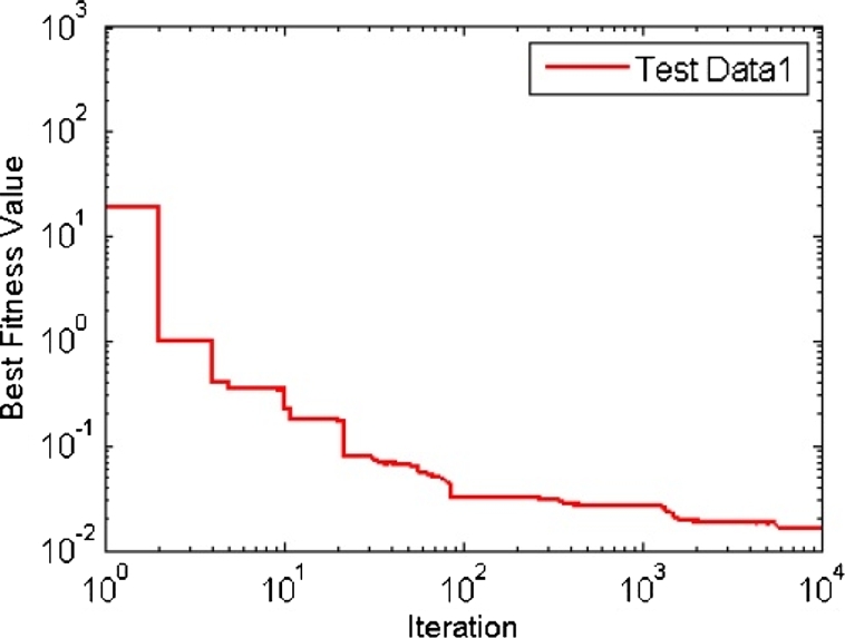
Convergence of fitness values for DS 1.

Table 2 shows that the proposed model has much better end-point prediction ability compare to NN, PSO and DWCM. PSO approach on PNSRNN has the most end-point predictive power at the end point result $E_8$. PNSRNN has the overall commanding ability for end-point prediction than PSO and NN. The end-point predictive competence of the proposed model increases with execution time. The model is developed by combining two of three models has a better end-point predictive power than the models that are developed by NN, PSO and DWCM. It is obvious that for all end point results, the NPSO approach has a better end-point prediction capability than ${\text{NN}}_{YP}$, ${\text{PSO}}_{YP}$, ${\text{NN}}_{YR}$, ${\text{PSO}}_{YR}$, ${\text{NN}}_{PR}$, ${\text{PSO}}_{PR}$, NN, PSO and DWCM.

Table 2.

Comparison of end point result of PNSRNN model for DS 1.

	NNYP	PSOYP	NNYR	PSOYR	NNPR	PSOPR	NN	PSO	DWCM	NPSO
E10	64.6795	49.1865	40.6612	37.6588	23.5535	31.6499	6.0170	0.6659	1.3082	0.0974
E9	48.7511	18.6534	26.9104	52.3012	6.5612	41.0519	3.4043	2.2461	1.1634	0.2679
E8	29.5798	28.3503	24.5119	47.8788	10.8851	21.5055	2.3177	5.2668	0.7847	0.2780
E7	44.1151	11.9057	17.0376	13.7094	15.6594	37.6405	3.2760	11.1002	2.9823	0.3293
E6	24.3763	20.2017	66.1641	17.0710	10.2457	17.5801	9.8850	8.6444	0.2759	0.3301
E5	31.5467	20.6991	24.2581	44.1102	34.8596	10.7967	13.9846	8.7973	1.7892	0.4233
E4	15.8331	27.4585	32.8564	15.3095	49.7422	28.1310	5.3551	9.9872	2.1241	0.4526
E3	30.6549	48.1234	19.9689	17.2630	18.4782	17.1943	6.8211	0.0230	3.5768	0.5503
E2	10.4981	17.9740	21.4475	17.1506	32.2898	26.3240	4.5263	2.9070	3.7622	0.6017
E1	18.3798	34.9055	18.8066	19.2588	30.8308	25.2519	9.2694	2.8378	6.8211	0.7035

Fig. 6 depicts that the proposed model has smaller RPEs than the DWCM, NN, PSO and other existing models. The PNSRNN has much lesser RPE which establish excellent software reliability.

Figure 6.

RPE curve of PNSRNN model for DS 1.

2.10. Performance measures for DS-2

The fitting of the proposed model to DS2 is presented in Fig. 7, which shows the plots of the actual fault compared with the predicted faults by the MVF of the proposed model.

Figure 7.

Graph of goodness of fit for DS 2.

Fig. 8 most effectively represents convergence graph for the NPSO during minimization of error generated from equation (6). It is training by failure data by DS-2 for PNSRNN model.

Figure 8.

Convergence of fitness values for DS 2.

The comparison of end point result of proposed PNSRNN model is presented in Table 3. The end point value of the proposed model improves from the iterations $E_1$ to $E_{10}$, and reached lowest end point value at $E_{10}$. The proposed model has better end-point prediction in $E_1$ to $E_8$. NPSO than NN, PSO and DWCM approach. NN approach on PNSRNN has the utmost end-point predictive ability at the End Point result $E_{10}$. The end point predictive powers are increased with the growth of execution time. The proposed model has best end point prediction by NPSO than NN, PSO an DWCM approach. NN approach has relative errors which are smallest from RE values of the model under comparison at end point result $E_{10}$ and $E_9$. It is obvious that for all end point results, the NPSO approach has better end-point prediction capability than ${\mathrm{NN}}_{YP}$, ${\mathrm{PSO}}_{YP}$, ${\mathrm{NN}}_{YR}$, ${\mathrm{PSO}}_{YR}$, ${\mathrm{NN}}_{PR}$, ${\mathrm{PSO}}_{PR}$, NN, PSO and DWCM.

Table 3.

Comparison of end point result of PNSRNN model for DS 2.

	NNYP	PSOYP	NNYR	PSOYR	NNPR	PSOPR	NN	PSO	DWCM	NPSO
E10	5.6995	15.5255	47.1979	11.2794	55.5481	23.6493	0.0339	2.0961	4.4062	0.7035
E9	6.9240	21.2094	25.0536	14.9242	68.3383	17.7973	0.0722	2.2683	9.5636	0.6017
E8	7.2148	21.2975	50.5329	20.9679	89.9163	19.7966	7.7064	2.2317	8.7395	0.5503
E7	8.6668	13.5990	10.2012	20.9744	22.6253	17.5909	9.0823	2.3781	1.8030	0.4526
E6	1.9116	12.8895	20.8446	22.3911	21.9341	25.0868	9.4334	2.3502	1.4151	0.4233
E5	8.1315	23.3555	55.2913	22.9715	15.7956	35.6900	10.5945	2.7509	1.7351	0.3293
E4	1.6968	16.7727	47.4991	24.8672	29.3671	32.1819	13.4800	3.3984	1.5121	0.3293
E3	13.3583	40.9834	9.0755	26.3564	31.2637	26.2597	13.1002	3.4485	2.3827	0.2780
E2	13.4882	36.5031	33.4176	27.4113	25.7005	59.1024	13.7118	3.5808	2.1301	0.2679
E1	13.4968	13.0277	27.0384	47.0330	14.8235	12.7002	13.3516	4.5355	4.8166	0.0974

Fig. 9 shows that the proposed model has smaller RPEs than the other than NN, PSO and DWCM. The PNSRNN has the lowest RPE compare to other models, i.e. the proposed PNSRNN has the best prediction capability than NN and PSO.

Figure 9.

RPE curve of PNSRNN model for DS 2.

2.11. Performance measures for DS-3

The fitting of the proposed model to the DS3 is presented in Fig. 10, which depicts the plots of the actual fault compared with the predicted faults, and the data is estimated by the MVF.

Figure 10.

Goodness of fit for DS 3.

Fig. 11 represents the graph of convergence for the proposed NPSO during minimization of error generated from equation (6). It is training by failure data by DS-3 of the recurrent NN for PNSRNN model.

Figure 11.

Convergence of fitness values for DS 3.

Table 4 shows that the proposed NPSO has much effective end-point prediction ability than the NN, PSO and DWCM. PNSRNN has the comprehensive effective end-point prediction capability than the NN, since the RE values of PSO are smallest under consideration of $E_5$. The PNSRNN based model has satisfactory end-point predictive capability compare to the models developed by NN, PSO and DWCM. It is obvious that for all end point results, the NPSO approach has better end-point prediction capability than ${\text{NN}}_{YP}$, ${\text{PSO}}_{YP}$, ${\text{NN}}_{YR}$, ${\text{PSO}}_{YR}$, ${\text{NN}}_{PR}$, ${\text{PSO}}_{PR}$, NN, PSO and DWCM.

Table 4.

Comparison of end point result of PNSRNN model for DS 3.

	NNYP	PSOYP	NNYR	PSOYR	NNPR	PSOPR	NN	PSO	DWCM	NPSO
E10	13.3809	81.6825	27.2272	46.3349	10.0241	15.0646	2.7035	2.2683	0.1443	0.0134
E9	32.1112	45.8041	51.9243	10.4390	62.6569	10.5335	7.1181	11.0462	0.1998	0.0137
E8	15.1254	40.0242	21.6906	32.9327	18.3568	21.0155	5.3891	2.2511	0.2019	0.1321
E7	86.1927	13.9221	20.3100	11.4459	10.7619	13.7515	2.5223	5.2331	0.2230	0.1279
E6	27.3174	30.5179	11.4434	47.8650	15.0571	19.3345	0.6116	8.5641	2.0258	0.1082
E5	10.8130	31.7522	15.4237	33.1725	13.3742	14.1085	7.8257	11.6885	0.2290	0.0472
E4	18.3703	18.0322	11.5300	22.6498	11.7402	12.0271	7.2761	0.0084	0.2383	0.0234
E3	23.6650	28.5335	16.6071	21.9761	17.4177	12.8271	2.7968	10.3322	0.3263	0.0384
E2	35.2454	98.8051	61.4583	31.5782	21.1460	10.3423	2.9338	3.9931	0.3518	0.3064
E1	26.7649	25.9798	29.0758	35.6507	19.8578	19.3188	9.6235	5.2129	0.3854	0.0675

Fig. 12 depicts the RPE curves of the proposed model have lower RPEs than the NN, PSO and DWCM. From the above figures and tables, we can conclude that NPSO approach provides a better prediction than NN, PSO and DWCM for PNSRNN model. The goodness of fit of PNSRNN model of the actual and predicted faults estimated by the MVF to all three test data (DS1, DS2 and DS3) are depicted in Figure 3, Figure 6, Figure 10 respectively. Figure 5, Figure 8, Figure 11 demonstrate the correlation between number of iteration and best fitness result for proposed PNSRNN Model.

Figure 12.

RPE curve for DS 3 of PNSRNN model.

2.12. Threats to validity

We have assimilated and generalized models to understand the issue in NHPP based modeling in this paper. In some cases, the fault introduction parameter in imperfect debugging is an inappropriate issue due to potentially complicated model. The proposed approach resolves most of the issues of different factors. We treated fault introduction rate by considering testing efficiency, testing team skill as additional parameter, and characteristic improvement among NHPP based SRGM modeling. The growth of introduced rate may be related to other factors such as efficiency of testing effort. In this work, we could not collect and evaluate the testing effort efficiency. The testing effort should influence the number of detected faults if test effort is not constant. Furthermore, the historical failure data sets are old enough to compare, and the scale of this system is smaller than the recent development. However, recent studies have also employed these data sets, which should protect the validity of the result of this study. We only tested proposed model with three data sets, which should protect the validity of the result of this study, but not sufficient to make uniform and/or generalized model. We also propose a two-stage Neighborhood PSO to escape the local maximal subject to fixing of issues up to a desired level.

3. Conclusions

This paper has presented a conceptually simple and efficient PSO algorithm within a supervised back-propagation recurrent neural network architecture. Adaptive inertia weights to train the neural network is employed by the NPSO algorithm. The algorithm is prevented from becoming trapped in local optima by the dynamic adaptive nature of the proposed NPSO. The algorithms were put into application in the context of assimilation of three well-known NHPP based SRGM for software reliability prediction. However, this approach can be applied for different applications in the many areas of engineering and science where s-shaped models are relevant. Three software failure data sets from the real time research literature were applied through the proposed NPSO algorithm. The experimental results showcased the exhibitions of better predictive quality by the NPSO than the PSO alone. The prospective of hybrid methods for prediction of software reliability with greater accuracy is thus illustrated by the combination of PSO and ANN based recurrent neural network.

The upcoming research will establish the framework of combination of NN architectures and PSO algorithms along with several other combinations of algorithms through different approaches. These different framework of combination will help for training of the failure data sets as well as for the capability of prediction of faults. Alternative soft computing approaches may be considered for the fitting and prediction under uncertainty of the flexibility logistic growth curve models along with several software reliability growth models.

Declarations

Author contribution statement

Pooja Rani, G.S. Mahapatra: Conceived and designed the experiments; Performed the experiments; Analyzed and interpreted the data; Contributed reagents, materials, analysis tools or data; Wrote the paper.

Funding statement

This research did not receive any specific grant from funding agencies in the public, commercial, or not-for-profit sectors.

Competing interest statement

The authors declare no conflict of interest.

Additional information

No additional information is available for this paper.

References

- 1.Littlewood B., Strigini L. The Future of Software Engineering. ACM Press; 2000. Software reliability and dependability: a roadmap. [Google Scholar]
- 2.Musa J.D. Faster Development and Testing. McGraw-Hill; 2004. Software reliability engineering: more reliable software. [Google Scholar]
- 3.Lyu Michael R. Future of Software Engineering. 2007. Software reliability engineering: a roadmap; pp. 55–71. [Google Scholar]
- 4.ANSI/IEEE . ANSI/IEEE; 1991. Standard Glossary of Software Engineering Terminology. STD-729-1991. [Google Scholar]
- 5.Pham H. Springer; 2006. System Software Reliability. [Google Scholar]
- 6.Yamada S., Osaki S. Software reliability growth modeling: models and applications. IEEE Trans. Softw. Eng. 1985;11:1431–1437. [Google Scholar]
- 7.Pham H., Normann L., Zhang Z. A general imperfect software debugging model with s-shaped detection rate. IEEE Trans. Reliab. 1999;48(2):169–175. [Google Scholar]
- 8.Hewett R. Mining software defect data to support software testing management. Appl. Intell. 2011;34(2):245–257. [Google Scholar]
- 9.Roy P., Mahapatra G.S., Dey K.N. An S-shaped software reliability model with imperfect debugging and improved testing learning process. Int. J. Reliab. Saf. 2013;7(4):372–387. [Google Scholar]
- 10.Chatterjee S., Maji B. A bayesian belief network based model for predicting software faults in early phase of software development process. Appl. Intell. 2018;48(8):2214–2228. [Google Scholar]
- 11.Huang C.Y., Lyu M.R., Kuo S.Y. A unified scheme of some nonhomogeneous Poisson process models for software reliability estimation. IEEE Trans. Softw. Eng. 2003;29(3):261–269. [Google Scholar]
- 12.Li S.M., Yin Q., Guo P., Lyu M.R. A hierarchical mixture model for software reliability prediction. Appl. Math. Comput. 2007;185:1120–1130. [Google Scholar]
- 13.Lai Richard, Garg Mohit. A detailed study of NHPP software reliability models. J. Softw. 2012;7(6):1296–1306. [Google Scholar]
- 14.Malaiya Y.K., Li M.N., Bieman J.M., Karcich R. Software reliability growth with test coverage. IEEE Trans. Reliab. 2002;51:420–426. [Google Scholar]
- 15.Liu Y., Li D., Wang L., Hu Q. A general modeling and analysis framework for software fault detection and correction process. Softw. Test. Verif. Reliab. 2016;26(5):351–365. [Google Scholar]
- 16.Hu Q.P., Xie M., Ng S.H., Levitin G. Robust recurrent neural network modeling for software fault detection and correction prediction. Reliab. Eng. Syst. Saf. 2007;92:332–340. [Google Scholar]
- 17.Roy P., Mahapatra G.S., Dey K.N. An NHPP software reliability growth model with imperfect debugging and error generation. Int. J. Reliab. Qual. Saf. Eng. 2014;21(02) [Google Scholar]
- 18.Wanga J., Wu Z. Study of the nonlinear imperfect software debugging model. Reliab. Eng. Syst. Saf. 2016;153:180–192. [Google Scholar]
- 19.Chandrasekharan S., Panda R.C., Swaminathan B.N. Statistical modeling of an integrated boiler for coal fired thermal power plant. J. Heliyon. 2017;3(6) doi: 10.1016/j.heliyon.2017.e00322. [DOI] [PMC free article] [PubMed] [Google Scholar]
- 20.Chatterjee S., Nigam S., Singh J.B., Upadhyaya L.N. Software fault prediction using Nonlinear Autoregressive with eXogenous Inputs (NARX) network. Appl. Intell. 2012;37(1):121–129. [Google Scholar]
- 21.Huang C.Y., Kuo S.Y. Analysis of incorporating logistic testing effort function into software reliability modeling. IEEE Trans. Reliab. 2002;51(3):261–270. [Google Scholar]
- 22.Goel A.L., Okumoto K. Time-dependent error-detection rate model for software reliability and other performance measures. IEEE Trans. Reliab. 1979;28(3):206–211. [Google Scholar]
- 23.Karunanithi N., Malaiya Y.K. Handbook of Software Reliability Engineering. McGraw-Hill; 1996. Neural networks for software reliability engineering; pp. 699–728. [Google Scholar]
- 24.Khoshgoftaar T.M., Szabo R.M. Predicting software quality, during testing, using neural network models: a comparative study. Int. J. Reliab. Qual. Saf. Eng. 1994;1:303–319. [Google Scholar]
- 25.Tian L., Noore A. Evolutionary neural network modeling for software cumulative failure time prediction. Reliab. Eng. Syst. Saf. 2005;87:45–51. [Google Scholar]
- 26.Zheng J. Predicting software reliability with neural network ensembles. Expert Syst. Appl. 2009;36:2116–2122. [Google Scholar]
- 27.Su Y.S., Huang C.Y. Neural-network-based approaches for software reliability estimation using dynamic weighted combinational models. J. Syst. Softw. 2007;80:606–615. [Google Scholar]
- 28.Kapur P.K., Khatri S.K., Basirzadeh M. Software reliability assessment using artificial neural network based flexible model incorporating faults of different complexity. Int. J. Reliab. Qual. Saf. Eng. 2008;15(2):113–127. [Google Scholar]
- 29.Kapur P.K., Goswami D.N., Bardhan A., Singh Ompal. Flexible software reliability growth model with testing effort dependent learning process. Appl. Math. Model. 2008;32(7):1298–1307. [Google Scholar]
- 30.Li Q., Pham H. NHPP software reliability model considering the uncertainty of operating environments with imperfect debugging and testing coverage. Appl. Math. Model. 2017;51:68–85. [Google Scholar]
- 31.Chuang Chun-Hsiang, Cao Zehong, Wang Yu-Kai, Chen Po-Tsang, Huang Chih-Sheng, Pal Nikhil R., Lin Chin-Teng. Dynamically weighted ensemble-based prediction system for adaptively modeling driver reaction time. IEEE Trans. Biomed. Eng. 2018 arXiv:1809.06675 [Google Scholar]
- 32.Rani P., Mahapatra G.S. Neural network for software reliability analysis of dynamically weighted NHPP growth models with imperfect debugging. J. Softw. Test. Verif. Reliab. 2018 [Google Scholar]
- 33.Sitte R. Comparison of software-reliability-growth predictions: neural networks vs parametric-recalibration. Trans. Reliab. 1999;48(3):285–291. Griffith Univ., Brisbane, Qld., Australia. [Google Scholar]
- 34.Kiran N.R., Ravi V. Software reliability prediction by soft computing techniques. J. Syst. Softw. 2008;81(4):576–583. [Google Scholar]
- 35.Mohanty R., Ravi V., Patra M.R. Hybrid intelligent systems for predicting software reliability. Appl. Soft Comput. 2013;13(1):189–200. [Google Scholar]
- 36.Awolusia T.F., Okea O.L., Akinkurolerea O.O., Sojobib A.O., Alukoa O.G. Performance comparison of neural network training algorithms in the modeling properties of steel fiber reinforced concrete. J. Heliyon. 2019;5(1) doi: 10.1016/j.heliyon.2018.e01115. [DOI] [PMC free article] [PubMed] [Google Scholar]
- 37.Xu G. An adaptive parameter tuning of particle swarm optimization algorithm. Appl. Math. Comput. 2013;219:4560–4569. [Google Scholar]
- 38.Eberhart R.C., Shi Y. Proceedings of the IEEE Evolutionary Computation, vol. 1. 2001. Tracking and optimizing dynamic systems with particle swarm; pp. 94–100. [Google Scholar]
- 39.Poli R., Kennedy J. Particle swarm optimization. Time BlackwellSwarm Intell. 2007;1(1):33–57. [Google Scholar]
- 40.Wanga H., Sun H., Li C., Rahnamayan S., Pan J. Diversity enhanced particle swarm optimization with neighborhood search. Inf. Sci. 2013;223:119–135. [Google Scholar]
- 41.Sun C., Zeng J., Pan J. An improved vector particle swarm optimization for constrained optimization problems. Inf. Sci. 2011;181(6):1153–1163. [Google Scholar]
- 42.Malhotra R., Negi A. Reliability modeling using particle swarm optimization. Int. J. Syst. Assur. Eng. Manag. 2013;4(3):275–283. [Google Scholar]
- 43.Rani P., Mahapatra G.S. A neuro-particle swarm optimization logistic model fitting algorithm for software reliability analysis. Proc. Inst. Mech. Eng., Part O: J. Risk Reliab. 2019 [Google Scholar]
- 44.Kansal Y., Choudhary S. Forecasting the reliability of software via neural networks. Int. J. Comput. Sci. Inf. Technol. 2014;5(2):2658–2661. [Google Scholar]
- 45.Kennedy J., Eberhart R. Proc. IEEE International Conference on Neural Networks. 1995. Particle swarm optimization; pp. 1942–1948. [Google Scholar]
- 46.Bai Q. Analysis of particle swarm optimization algorithm. Comput. Inf. Sci. 2010;3(1):180–184. [Google Scholar]
- 47.Eberhart R.C., Shi Y. Comparing inertia weights and constriction factors in particle swarm optimization. IEEE Evol. Comput. 2000;1:84–88. [Google Scholar]
- 48.Nasir M., Das S., Maity D., Sengupta S., Halder U., Suganthan P.N. A dynamic neighborhood learning based particle swarm optimizer for global numerical optimization. Inf. Sci. 2012;209:16–36. [Google Scholar]
- 49.Mousa A.A., El-Shorbagy M.A., Abd-El-Wahed W.F. Local search based hybrid particle swarm optimization algorithm for multiobjective optimization. Swarm Evol. Comput. 2012;3:1–14. [Google Scholar]
- 50.Jin C., Jin S.W. Parameter optimization of software reliability growth model with S-shaped testing-effort function using improved swarm intelligent optimization. Appl. Soft Comput. 2016;40:283–291. [Google Scholar]
- 51.Truong V.H., Kim S.E. Reliability-based design optimization of nonlinear inelastic trusses using improved differential evolution algorithm. Adv. Eng. Softw. 2018;121:59–74. [Google Scholar]
- 52.Tian M., Gao X. Differential evolution with neighborhood-based adaptive evolution mechanism for numerical optimization. Inf. Sci. 2019;478:422–448. [Google Scholar]
- 53.Huang C.L. A particle based simplified swarm optimization algorithm for reliability redundancy allocation problems. Reliab. Eng. Syst. Saf. 2015;142:221–230. [Google Scholar]
- 54.Wang J., Wu Z., Shu Y., Zhang Z. An optimized method for software reliability model based on nonhomogeneous Poisson process. Appl. Math. Model. 2016;40:6324–6339. [Google Scholar]
- 55.Roy P., Rani Pooja, Mahapatra G.S., Pandey S.K., Dey K.N. Robust feedforward and recurrent neural network based dynamic weighted combination models for software reliability prediction. Appl. Soft Comput. 2014;22:629–637. [Google Scholar]
- 56.Roy P., Mahapatra G.S., Dey K.N. Neuro-genetic approach on logistic model based software reliability prediction. Expert Syst. Appl. 2015;42(10):4709–4718. [Google Scholar]
- 57.Bansal J.C., Singh P.K., Saraswat M., Verma A., Jadon S.S., Abraham A. Inertia weight strategies in particle swarm optimization. Proc. IEEE Nature and Biologically Inspired Computing (NaBIC); Salamanca; 2011. pp. 19–21. [Google Scholar]
- 58.Cai K.Y., Cai L., Wang W.D., Yu Z.Y., Zhang D. On the neural network approach in software reliability modeling. J. Syst. Softw. 2001;58:47–62. [Google Scholar]
- 59.Xiaonan Z., Junfeng Y., Siliang D., Shudong H. A new method on software reliability prediction. Math. Probl. Eng. 2013 [Google Scholar]
- 60.Ramasamy Subburaj, Deiva Preetha C.A.S. Dynamically weighted combination model for describing inconsistent failure data of software projects. Indian J. Sci. Technol. 2016;9(35) [Google Scholar]
- 61.Huang C.Y., Kuo S.Y. Proc. the Eighth International Symposium on Software Reliability Engineering. 1997. Analysis of a software reliability growth model with logistic testing-effort function; pp. 378–388. [Google Scholar]
- 62.Roy P., Mahapatra G.S., Dey K.N. An efficient particle swarm optimization-based neural network approach for software reliability assessment. Int. J. Reliab. Qual. Saf. Eng. 2017;24(4) [Google Scholar]