Structural Variability in the Human Brain Reflects Fine-Grained Functional Architecture at the Population Level

Abstract

Human brain structure topography is thought to be related in part to functional specialization. However, the extent of such relationships is unclear. Here, using a data-driven, multimodal approach for studying brain structure across the lifespan (N = 484, n = 260 females), we demonstrate that numerous structural networks, covering the entire brain, follow a functionally meaningful architecture. These gray matter networks (GMNs) emerge from the covariation of gray matter volume and cortical area at the population level. We further reveal fine-grained anatomical signatures of functional connectivity. For example, within the cerebellum, a structural separation emerges between lobules that are functionally connected to distinct, mainly sensorimotor, cognitive and limbic regions of the cerebral cortex and subcortex. Structural modes of variation also replicate the fine-grained functional architecture seen in eight well defined visual areas in both task and resting-state fMRI. Furthermore, our study shows a structural distinction corresponding to the established segregation between anterior and posterior default-mode networks (DMNs). These fine-grained GMNs further cluster together to form functionally meaningful larger-scale organization. In particular, we identify a structural architecture bringing together the functional posterior DMN and its anticorrelated counterpart. In summary, our results demonstrate that the relationship between structural and functional connectivity is fine-grained, widespread across the entire brain, and driven by covariation in cortical area, i.e. likely differences in shape, depth, or number of foldings. These results suggest that neurotrophic events occur during development to dictate that the size and folding pattern of distant, functionally connected brain regions should vary together across subjects.

SIGNIFICANCE STATEMENT Questions about the relationship between structure and function in the human brain have engaged neuroscientists for centuries in a debate that continues to this day. Here, by investigating intersubject variation in brain structure across a large number of individuals, we reveal modes of structural variation that map onto fine-grained functional organization across the entire brain, and specifically in the cerebellum, visual areas, and default-mode network. This functionally meaningful structural architecture emerges from the covariation of gray matter volume and cortical folding. These results suggest that the neurotrophic events at play during development, and possibly evolution, which dictate that the size and folding pattern of distant brain regions should vary together across subjects, might also play a role in functional cortical specialization.

Introduction

A long-standing concept postulates that functional specialization of the cortex relates to the cytoarchitectony and pattern of convolutions in the cortex of mammals with folded brains (Toro and Burnod, 2005). However, the extent to which structural and functional architectures in humans might map onto one another remains unclear. Recently, fMRI studies have shown that the functional organization of the brain is shaped by an intrinsic architecture that can be observed in the network patterns of both task-related and resting fMRI (Smith et al., 2009; Finn et al., 2015). Additional evidence has now begun to suggest that such functional architecture topographically corresponds to an equivalent network-based structural organization, with particular networks found to occur both in functional and structural imaging (Greicius et al., 2009; Honey et al., 2009; Segall et al., 2012; Alexander-Bloch et al., 2013; Sporns, 2014). For instance, “structural covariance” studies, in which maps of covariation in the size of gray matter regions at a population level are created using regions of interest, have revealed gray matter architectures partly resembling intrinsic functional resting-state networks (RSNs) (Chen et al., 2008; Seeley et al., 2009). In addition, identification of patterns in healthy brain structure have recently provided insights into the spread and selective targeting of disease processes, making an understanding of these structural networks highly relevant to the clinical field (Seeley et al., 2009; Raj et al., 2012; Douaud et al., 2014; Zeighami et al., 2015).

However, fundamental questions remain unanswered on the extent and nature of this structure–function correspondence. For example, the following remain to be determined: (1) whether gray matter volume structural covariance patterns reflect the entire repertoire of canonical functional architecture; that is, whether all of the brain regions present in canonical functional networks also covary in size across the population; (2) if structure–function correspondence can be detected at a finer degree of detail than those canonical functional networks; and (3) if such volume variation across subjects is associated with variation in the folds and thickness of the cortex.

To uncover the richness of structural patterns in the human brain, we investigate here the gray matter structure of a large healthy population covering most of the lifespan (8–85 years) with a data-driven approach. Using one structural MRI scan per subject, our multimodal approach (linked independent component analysis) (Groves et al., 2011) makes it possible to co-model three types of gray matter information to reveal maps of population covariation in gray matter volume, as well as complementary maps of covariation in cortical area and cortical thickness to help disentangle the possible interpretations of gray matter volume results. We decomposed the data into 70 modes of variation—or independent components (ICs)—to allow further comparison with the functional network decompositions presented in (Smith et al., 2009) that showed good correspondence between resting and task-related networks. Each of the spatial ICs obtained with this method represents a mode of covariation of gray matter volume, area, and thickness across all 484 participants.

Materials and Methods

Participants and imaging protocol.

A total of 484 right-handed healthy volunteers (264 females) covering most of the lifespan (aged 8 to 85 years, 39 ± 13 years) were included in this study from two separate research projects run by the Research Group for Lifespan Changes in Brain and Cognition at the University of Oslo (“Neurocognitive Development” and “Cognition and Plasticity through the Life-Span”). The study was approved by the Regional Committee for Medical and Health Research Ethics in Norway. More information about inclusion and exclusion criteria can be found in Douaud et al. (2014).

All participants underwent the same imaging protocol on a 1.5 T Siemens Avanto scanner at Oslo University Hospital, with no hardware upgrades and only minor software upgrades performed during the course of the acquisition period (2006–2010). Whole-brain T1-weighted images were acquired using a 12-channel head coil and magnetization prepared rapid gradient echo (MPRAGE) with the following parameters: TR/TE/TI = 2400/3.61/1000 ms, flip angle of 8°, matrix 192 × 192, FOV 240 mm, voxel size 1.25 × 1.25 × 1.2 mm³, 160 sagittal slices. To increase signal-to-noise ratio, the sequence was run twice within a single session.

Imaging processing.

As we aim to further our understanding of what the contributing factors to the gray matter volume networks might be, for example, as described in Seeley et al. (2009), we assessed cortical thickness and area in addition to volume, as these are the two modalities typically used to disentangle the different contributions to, and possible interpretations of, gray matter volume in numerous previous studies (Douaud et al., 2007; Voets et al., 2008; Jalbrzikowski et al., 2013; Storsve et al., 2014; Winkler et al., 2018).

T1-weighted images were processed using FSL-VBM (Douaud et al., 2007), an optimized voxel-based morphometry analysis protocol (Ashburner and Friston, 2000) using FMRIB Software Library (FSL) tools (fsl.fmrib.ox.ac.uk/fsl/fslwiki/FSLVBM) (Smith et al., 2004). For each subject, the input image for FSL-VBM was an average of the two coaligned MPRAGE scans. The two runs were preprocessed using FreeSurfer (http://surfer.nmr.mgh.harvard.edu/), including motion correction, averaging, and intensity nonuniformity correction. Before the FSL-VBM processing, the volumes were masked by the full-brain segmented volume output from FreeSurfer (Fischl et al., 2002), excluding nonbrain compartments. A left–right symmetric, study-specific template was created by: (1) registering the 484 brain-extracted, gray matter-segmented images to the MNI 152 standard space “avg152T1_gray” template using nonlinear registration and (2) averaging and flipping the resulting images along the x-axis. After nonlinearly normalizing all the gray matter images onto this symmetric study-specific gray matter template, the modulated registered gray matter images were smoothed with an isotropic Gaussian kernel with a σ of 2 mm (∼5 mm FWHM).

In addition, brain structural information was derived from two additional, complementary types of gray matter information: vertexwise cortical thickness and surface area measures calculated using FreeSurfer by means of an automated surface reconstruction scheme (Dale et al., 1999; Fischl et al., 1999; Fischl and Dale, 2000). Cortical thickness measurements were obtained by reconstructing representations of the gray/white boundary and the pial surface and then by calculating the distance between the surfaces at each vertex across the cortical mantle. Surface area was estimated by registering each subject's reconstructed surfaces to a common template (using folding information to drive the within-surface warping) and the relative amount of expansion or compression at each vertex was used as a proxy for regional area. These FreeSurfer maps were resampled, mapped to a common coordinate system using a nonrigid high-dimensional spherical averaging method to align cortical folding patterns, and smoothed with a Gaussian kernel with an FWHM of 10 mm.

Linked IC analysis (ICA).

Linked ICA is a data-driven approach that can co-model multiple imaging modalities. Its main goal is to model the imaging data as a set of interpretable ICs, characterizing plausible modes of variability across all subjects' modalities. Multimodal and data-driven aspects of such methods (linked ICA, but also joint ICA) have made these tools increasingly popular, especially in mental health disorders (Sui et al., 2011; Stephen et al., 2013; Francx et al., 2016; Doan et al., 2017b), where there is a strong heterogeneity in symptoms, disease course, and biological underpinnings (Marquand et al., 2016), but also recently with Alzheimer's disease and mild cognitive impairment (Doan et al., 2017a). Linked ICA is part of FSL (http://fsl.fmrib.ox.ac.uk/fsl/fslwiki/FLICA), and was described in detail in earlier FLICA papers (Groves et al., 2011; Douaud et al., 2014). Briefly, we ran the linked ICA decomposition on the 4D files obtained from our FSL-VBM and FreeSurfer processing (GM_mod_merg_s2_4 mm.nii.gz, ?h.thick.fsaverage5.10.mgh, ?h.pial.area.fsaverage5.10.mgh) with 70 ICs to make this comparable to the decomposition of resting-state and task-based fMRI datasets used in Smith et al. (2009) and n = 1000 maximum iterations. FLICA, which will eliminate unneeded components using Bayesian model order selection, kept all 70 ICs.

We identified all of the 70 ICs' spatial distributions using, wherever relevant, the Jülich atlas, based on probabilistic cytoarchitectonic segmentations performed by the team of Professors Zilles and Amunts and transformed into MNI space (Eickhoff et al., 2005), as well as a cerebellum probabilistic atlas (Diedrichsen et al., 2009) devised using anatomical labels and boundaries defined postmortem (Schmahmann, 2000).

Post hoc association with age.

The result of the linked ICA is blind to the participants' demographics and solely relies on the information of the structural scans. We thus determined post hoc which ICs might show association (linear, quadratic, and cubic) with age (MATLAB2012, using glmfit). Results were corrected for multiple comparisons across all 70 ICs.

Spatial cross-correlation with resting-state and BrainMap networks.

Matching networks is a notoriously challenging task. Spatial correlation can objectively quantify how similar the topographical distribution across maps is (Smith et al., 2009; Douaud et al., 2014), but ultimately manual inspection is needed to help identifying maps as corresponding to the “canonical” DMN, executive, frontoparietal, visual, sensorimotor, and auditory networks (Beckmann et al., 2005). The level of fragmentation can also vary across datasets. Here, to compare the spatial distribution of the gray matter networks (GMNs) with those of the canonical functional networks, we adopted the approach of normalizing and averaging across networks when the level of fragmentation was higher for one dataset. We considered a whole gray matter mask and correlated all voxels of the FLICA relevant ICs with both resting-state fMRI (RSN) and the BrainMap (BM) fMRI database (Fox and Lancaster, 2002) canonical functional networks from Smith et al. (2009) using voxelwise spatial cross-correlation. To assess the significance of the spatial cross-correlations between the structural and functional ICs, we randomly generated 1000 Gaussian noise images that we smoothed with the corresponding estimated smoothness for each set of ICs. We then calculated the 1000 cross-correlations between each pair of these ICs and compared the strength of our observed correlations with this empirically generated null distribution.

Hierarchical clustering between the structural components.

We used hierarchical clustering to investigate whether 36 of the most identifiable structural network ICs would form together functionally meaningful higher-order clusters. We used the correlation coefficient of the subject-weight vectors between any two ICs as similarity measure, and complete linkage as an algorithm to create the cluster tree in MATLAB version 7.14. In the hierarchical tree, the height of each inverted U links represents the distance (here 1 − r) between the two objects being connected. Hierarchical clustering on the transposed matrix, that is, using the correlation coefficient between the ICs distribution of subjects' weights for two given subjects, revealed no pattern in the grouping of the subjects that could be associated with demographics or cognitive measures.

The sub-Gaussian nature of the more spatially extended (global) components retained by FLICA and the rich complementarity between the different measures derived from the T1 data (volume, area, thickness) might explain why our linked ICA approach performed so well with respect to identifying many—and functionally linked—distinct components of covariation: for instance, in a previous study of just gray matter “concentration,” six of 75 ICs were identified for network correlations to be compared here with 36 of 70 ICs that were included in our hierarchical clustering analysis (Segall et al., 2012). Although the multimodality of gray matter information resulted in clearer, more spatially well defined results and facilitated their interpretability, running FLICA (with the same set of options) solely based on the gray matter volume information yielded similar results (data not shown).

Replication.

As an accessible replication sample covering this large age range is not readily available, we empirically demonstrated the robustness of our findings via a split-half procedure. We split the 484 subjects into two groups of equal size (n = 242) perfectly age matched in mean and in variance to the original population and to one another (to retain what we believe is an important feature of our original population, mean: 39.4 ± 22.6 years of age), and ran FLICA with the same options on these two subgroups. We identified the two new sets of ICs by comparing them with the original analysis using voxelwise spatial cross-correlation, following the same procedure described above, and then compared the two new sets of ICs with one another.

The results and script are available at: http://www.fmrib.ox.ac.uk/datasets/FLICA_ThickAreaVol/. This experiment has not been preregistered.

Results

Global and age-related independent components

Of the 70 ICs, there were three global, spatially nonspecific components accounting for most of the structural variance across all the 484 healthy participants. IC1 was a multimodal component made of 51% cortical thickness information (accounting, in this specific IC, for 65% of the cortical thickness variance across all the participants), 7% cortical area (accounting for 17% of the cortical area variance), and 42% gray matter volume (accounting for 49% of the gray matter volume variance) (Douaud et al., 2014). IC2 was essentially composed of cortical area information (89%, accounting for 27% of the variance) and IC3 of cortical thickness (98%, accounting for 10%).

Overall, 13 ICs were statistically significantly associated with age either quadratically (n = 6: IC4, 6, 9, 18, 19, 24), cubically (n = 5: IC11, 49, 50, 52, 67), quadratically and cubically (n = 1: IC5), or all three (n = 1: IC1), after correction for multiple comparisons. However, only two of these ICs showed also practical significance for these associations, that is, significance measured using effect magnitude, such as the variance explained by age, as opposed to p-values (Kirk, 1996): IC1 and IC4, comprehensively described previously (Douaud et al., 2014). Six ICs showed significant sex-related differences after correction for multiple comparisons, although only three ICs remained associated with sex after adjusting for intracranial volume and only one IC considering practical significance: IC4 (Douaud et al., 2014).

Four modes of structural variability were artifactual components: IC6 related to the variable efficacy of the brain extraction around the basal arteries and IC9, IC19, and IC63 were dominated by only a few of the participants' scans (between 1 and 3), although such ICs might still represent an anatomically meaningful mode of variability for the remaining participants. For instance, one of them defined precisely the basal ganglia structures, but seemed very strongly driven by one elderly subject exhibiting numerous Virchow–Robin spaces in those structures. It is altogether possible, however, that the remaining 483 participants' contribution to this IC might have been valuable because, of the 70 ICs, no other one revealed mode of variation in the basal ganglia. By contrast, another structural covariance study found the strongest spatial cross-correlation with functional networks in the basal ganglia (Segall et al., 2012).

GMNs

The vast majority of the remaining structural components (∼40 of the 70 ICs) represented regional patterns of mostly spatially covarying gray matter volume and cortical area recapitulating functionally meaningful networks across the entire brain (see Figs. 1 and 2 and for more details of these networks, see below). These components describing localized, well defined modes of variation showed no relationship with age (linear, quadratic, or cubic), sex, intracranial volume, or education after correction for multiple comparisons. Each of these “GMNs” explained a small amount of the structural variance (Table 1), as most of such variance (and age relationship) was accounted for in the first three global components that together explained 76% of the variance in cortical thickness, 44% in area and 50% in volume (see above). Indeed, these GMNs inherently described modes of variation over and above variation associated with all other components, including the strongly age-related IC1 and IC3, which are widespread components of gray matter volume and cortical thickness. These GMNs covered the entire brain and offered a fine-grained, winner-take-all parcellation with almost 500 areas in total (using spherical connectivity; ∼200 with > 20 voxels) (Fig. 2). These parcels revealed, for instance, a clear separation between BA44 and BA45 (Amunts et al., 1999) or between PF and PG in the inferior parietal cortex (Caspers et al., 2006) despite cytoarchitectonic borders between adjacent association cortices (such as in these two cases) being considerably more subtle than in primary areas (Fischl et al., 2008), as well as between crus I and II in the cerebellum (see more details below) (Diedrichsen et al., 2009).

Figure 1.

GMNs map onto canonical functional networks identified in Smith et al. (2009) in both rest and task fMRI. The GMNs (GMNs, left in each panel) spatially correspond to the previously matched functional networks obtained using a data-driven approach (RSNs, middle of each panel; BrainMap task-related fMRI networks, obtained from nearly 30,000 subjects: BM, right in each panel). Due to a higher degree of fragmentation in the structural data, we averaged the two structural DMNs, DMN 1 and DMN 2, and the three structural sensorimotor networks. The spatial correlation coefficients obtained between GMNs and a given set of functional networks were mainly consistent with those observed between the two functional datasets (Table 2). By radiological convention, left is right in all figures.

Figure 2.

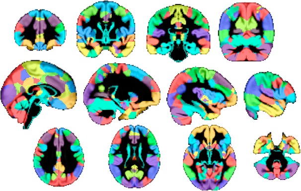
Parcellation across the entire brain based on the structural GMNs. Hard parcellation (winner-take-all) created using the absolute z maps for the 36 structural GMNs used in the hierarchical clustering analysis, semitransparent and overlaid onto the gray matter average across all 484 participants. Note the bilateral aspect of most networks, except in the frontoparietal networks (top row, fourth right for parietal node; bottom row, second right for frontal node).

Table 1.

Variance explained by each of the GMNs (%)

IC number	CT	CA	VOL	GMNs
8	0.4	2.3	1.0	Visual 1
11	0.1	1.5	1.2	Executive
12	0.0	0.0	2.0	Cerebellum 3 (crus I versus crus II)
13	0.1	1.0	1.4	Visual 2
14	0.3	2.0	0.7	Auditory
15	0.5	1.2	0.9	Visual 3
17	0.1	1.1	1.3	DMN 1
18	2.6	0.0	0.0	Sensorimotor (M1, premotor), CT
20	0.4	0.8	1.1	Language
21	0.1	1.6	1.0	Other visual/motor (supplementary eye field)
22	0.0	1.8	0.8	Precentral versus inferior frontal gyrus
23	0.3	0.4	1.3	Visual 6
25	0.0	0.0	1.6	Cerebellum 1
28	0.2	0.2	1.1	Frontoparietal (parietal) R
29	0.6	0.8	0.3	Sensorimotor 1 (lateral: M1, premotor)
30	0.2	1.3	0.4	Sensorimotor 2 (lateral: sensory)
31	0.0	1.8	0.5	Frontoparietal (frontal) L
32	0.0	1.1	0.7	Visual 4
34	0.0	1.1	0.7	Oculomotor 1 (frontal/premotor/cingulate eye field)
35	0.1	0.8	0.8	Other visual (parieto-occipital fissure)
36	0.0	0.8	0.8	Sensorimotor 3 (medial)
40	0.1	0.8	0.8	Middle temporal sulcus
42	0.1	0.6	0.7	DMN 2
43	1.3	0.1	0.2	Auditory, CT
45	0.3	0.6	0.6	Olfactory (piriform)
46	0.2	0.8	0.5	Posterior superior temporal sulcus
47	0.1	0.9	0.5	Other visual (fusiform area: occipital)
48	0.0	0.0	1.0	Frontoparietal (parietal) L
49	0.0	0.0	1.0	Cerebellum 2
51	0.1	1.1	0.3	Visual 7
54	0.0	0.0	0.9	Visual 8
55	0.0	1.0	0.5	Frontoparietal (frontal 1) R
57	0.0	0.6	0.6	Visual 5
60	0.1	1.2	0.2	Frontoparietal (frontal 2) R
64	0.1	1.2	0.3	Oculomotor 2 (posterior supplementary eye field)
69	0.0	0.0	0.7	Cerebellum 4
Total variance	8.3	30.7	28.3

CT, Cortical thickness; CA, cortical area; VOL, grey matter volume. In total, the most identifiable networks explain about 8% of the variance in CT, 31% of CA, and 28% of VOL, as most of the variance is captured in the first three “global” ICs: 76% for CT, 44% for CA, and 50% for VOL.

The average map across all these GMNs revealed that the most shared brain regions were the dorsal lateral prefrontal cortex (particularly on the right), Broca's area (BA45, particularly on the left), supplementary motor area, posterior intraparietal sulcus, precuneus, Wernicke's area (OP1, mainly on the left), angular and midtemporal gyrus, temporal pole, fusiform gyrus, and V5/MT (mainly on the left) (Fig. 3). These mostly associative, transmodal regions (Mesulam, 1998) seem to spatially correspond to those which have been consistently found to be the most structurally connected nodes using white matter connectivity, most particularly the precuneus and intraparietal sulcus (Sporns, 2014). In other words, the regions that emerged from the FLICA decomposition the most often across all the GMNs in this healthy population are also the regions that share the most white matter connections to other parts of the brain (“hubs”) (Hagmann et al., 2008; Gong et al., 2009; Nijhuis et al., 2013). A future approach to directly test this hypothesis would be to concurrently run FLICA on gray matter information and white matter connectivity, as opposed to voxelwise diffusion measures, which only reveal very localized covarying effects in the subjacent white matter (Groves et al., 2012). Although these most-shared gray matter nodes show some similarities with the cortical hubs defined from “myelination” (T1w/T2w) maps in the same subjects (Broca's areas, angular gyrus, temporal pole, V5/MT on the left), the absence of the precuneus in these T1w/T2w images is conspicuous, demonstrating the complementarity of gray matter and cortical myelination information (Grydeland et al., 2019). These most-shared gray matter areas also display a very different pattern from that found when looking at the main nodes of structural differences between healthy subjects and those with a variety of brain disorders (Cauda et al., 2018). This transdiagnostic VBM meta-analysis obtained from BrainMap indeed revealed that the main areas of structural alterations were located in subcortical structures and the insula, as well as the anterior cingulate cortex. These gray matter areas therefore mostly describe the salience network, probably as a direct consequence of having a higher representation of schizophrenia and other mental health disorders in the meta-analysis (Goodkind et al., 2015).

Figure 3.

Most shared gray matter regions across all structural GMNs. This shows that, on average, the most present brain regions across all GMNs (present in > 10 ICs) are mainly the precuneus, the fusiform area (particularly on the right), the posterior intraparietal sulcus, and the (right) DLPFC (in red). The average z map is semitransparent and overlaid onto the gray matter average across all 484 healthy participants (|z| < 1.5).

Structural networks arise from the covariation of gray matter volume and cortical area

One key advantage of our linked ICA approach was its multimodal aspect, integrating gray matter volume, cortical area, and cortical thickness information simultaneously. This multimodal feature revealed that modes of variation in gray matter volume across participants mainly colocalized with modes of variation in cortical area; that is, presumably differences in shape, depth or number of foldings (Fig. 4). Gray matter volume networks involving primary sensory and motor areas such as V1, M1, S1, or A1 also partially covaried with local cortical thickness, perhaps as a result of being highly myelinated cortical regions (Fig. 5). Except in those primary sensory regions, thickness contributed little to those most interpretable GMNs and/or was below threshold. As mentioned above, by construction, our data-driven approach reveals these GMNs as modes of variation beyond age-related, more spatially widespread ICs (the majority of which were driven by cortical thickness). This likely explains differences with thickness studies (Chen et al., 2008), where a seed-based approach showed correlations between cortical regions that may have been age-mediated to some extent.

Figure 4.

Gray matter volume networks covary with regional, colocalized cortical area. The vast majority of the well identified cerebral gray volume networks covaried with regional cortical area; that is, both gray matter volume and colocalized cortical area variations appeared in the same IC. In this figure, we show the example of the executive GMN, DMN 1, and visual 4. For each example, gray matter volume is on the left (red-yellow), and colocalized cortical area on the right (red-yellow) (z > 5, cortical thickness did not pass the threshold). The medial aspect of the GMNs in general was not reproduced as well in the cortical area (often just below threshold), possibly suggesting that the reconstruction of the medial surface is more problematic than for the lateral hemisphere in FreeSurfer. Cortical area is projected in volume (an approximation) and smoothed with a Gaussian kernel of 1.5 mm σ for better visualization.

Figure 5.

Gray matter volume networks covary with cortical area and cortical thickness in primary sensory areas. Although the majority of the cerebral gray matter volume networks mainly covaried with cortical area, some ICs also showed a substantial contribution of cortical thickness in primary sensory areas. Here, we show the example of the auditory GMN and one of the sensorimotor GMNs. For both examples, gray matter volume is on the left, colocalized cortical area in the middle, and colocalized cortical thickness on the right (z > 5). Cortical area and thickness are projected in volume and smoothed with a Gaussian kernel of 1.5 mm σ for better visualization.

GMNs follow a functionally meaningful architecture

The functionally relevant level of detail described by these GMNs actually extended beyond the coarse spatial organization described by the canonical RSNs; that is, those most consistently described in the literature and that are common to both rest and task fMRI (Beckmann et al., 2005; Smith et al., 2009). By decomposing fMRI data into a higher number of dimensions or by using very localized regions of interest, studies have demonstrated that single RSNs can be consistently broken down into more detailed functional subnetworks (Margulies et al., 2009; Smith et al., 2009). Similarly, the GMNs in our study exhibited functionally meaningful fragmented organization, supporting the idea of a fine-grained correspondence between structural and functional architectures.

A these GMNs covered all of the canonical RSNs, they showed in most cases a higher degree of fragmentation. We identified for instance: (1) four cerebellum networks (cerebellum 1–4; Fig. 6); (2) eight visual networks (visual 1–8; Fig. 7); (3) two default-mode networks (DMN 1 and DMN 2; Fig. 8); (4) an executive network (Figs. 1 and 4); (5) three primary sensorimotor networks split into lateral primary sensorimotor cortex centered around BA3 and BA 4 (SMN 1), BA 1 and BA2 (SMN 2), as well as the medial sensorimotor cortex (SMN 3) (Geyer et al., 1996, 2000) (Figs. 1 and 5); (6) an auditory network (Figs. 1 and 5); (7) two left frontoparietal networks split into frontal and parietal unilateral networks (Fig. 9); and (8) two right frontoparietal networks, similarly split (Fig. 9).

Figure 6.

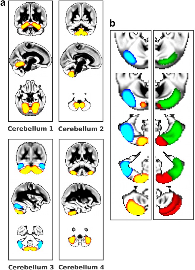
Fine-grained, functionally meaningful cerebellar gray matter architecture. a, The four cerebellar GMNs correspond to functionally different parts of the cerebellum and have distinct functional connectivity with the cerebral cortex (Sang et al., 2012) (z > 5). b, Left, Magnification of cerebellum 3 showing a clear distinction between crus I (blue) and crus II and VIIb (red-yellow); right, lobule VII from an anatomical cerebellar probabilistic atlas (Diedrichsen et al., 2009): crus I (in green), crus II and VIIb (in red).

Figure 7.

Fine-grained visual gray matter architecture matches that of rest and task fMRI. The eight visual GMNs correspond to those functional visual networks common to both task and rest fMRI presented in Smith et al. (2009) (z > 5, except in visual 7, in which z > 3). For each GMN, top right insert shows Smith et al. corresponding visual functional networks for the same coordinates: left, from rest fMRI, right from task fMRI, z > 3. Each structural–functional correspondence p < 10⁻³, see Table 3. For easier visualization, only the volume-based modality of the structural modes of variation is overlaid onto the gray matter average across all 484 participants.

Figure 8.

Functionally meaningful separation between anterior and posterior DMNs in the gray matter structure. These two DMN GMNs (left, z > 5) correspond to the well known functional connectivity patterns of cognitive (posterior, DMN 1) and limbic (anterior, DMN 2) precuneus (Margulies et al., 2009). This segregation also corresponds to a natural division in the BrainMap (BM, right z > 3) task-related fMRI database observed at higher dimension decomposition (Smith et al., 2009). When combined, the two gray matter DMNs spatially match the canonical functional DMN identified in both rest and task fMRI at lower dimensionality (p < 10⁻³, Table 2).

Figure 9.

Hierarchical clustering of GMNs reveals functionally meaningful higher-order organization. Left, Dendrogram representation of the clusters: the shorter the distance (1 − r) between each mode of variation is, that is, the height of the inverted U-shaped colored lines linking each mode, the stronger and the more meaningful their connection (only clusters linked by a distance <1 were considered). Right, We included in this hierarchical clustering analysis 36 of the most identifiable GMNs and present here one modality (volume) and one view only for easier visualization (except cortical thickness in M1, orange cluster; z > 5, except visual 7, yellow cluster, and the 2 ICs in M1, orange cluster, all at z > 3).

In particular, we found within the cerebellum a notable, functionally meaningful separation between the mainly sensorimotor lobules (I–VI), the cognitive lobules VII and VIIIa (with a clear delineation of crus I and II) and lobules VIIIb and IX, including the corresponding vermis (Fig. 6). In the visual cortex, we also identified the same fine detailed architecture as seen in functional data. Specifically, we identified in the GMNs the same eight visual functional networks identified both at rest and during task (Smith et al., 2009) (Fig. 7). We also replicated the separation of the DMN into anterior and posterior subnetworks that are well established in functional data (Uddin et al., 2009; Leech et al., 2011) (Fig. 8).

Remarkably, the spatial distribution of these GMNs was quantitatively very comparable to their rest and task fMRI counterparts (Smith et al., 2009) (Fig. 1, Tables 2, 3). Due to the higher degree of fragmentation in the structural data, we averaged the two structural DMN 1 and DMN 2 to compare them with the canonical functional DMN and averaged the three SMN 1–3 networks for comparison with the canonical functional sensorimotor network. This yielded spatial correlation coefficients that were mainly consistent with those observed between the two functional datasets (Table 2). Next, we also compared the spatial distribution of the eight visual GMNs and the eight rest and task functional networks that had been matched previously (Smith et al., 2009). We found that there was in general a strong, and sometimes indeed even stronger, spatial correspondence between structural networks and one set of functional networks (mostly the task-derived networks) than between the two sets of functional networks (Table 3).

Table 2.

Spatial correlation between structural and functional canonical networks (p < 10⁻³)

Canonical network	Spatial correlation (r)
	GMN/BM	GMN/RSN	BM/RSN
Default-mode network	0.47	0.47	0.63
Cerebellum network	0.66	0.20*	0.50
Sensorimotor network	0.38	0.52	0.58
Auditory network	0.56	0.40	0.46
Executive network	0.44	0.40	0.27
Frontoparietal network (left)	0.26	0.22	0.58
Frontoparietal network (right)	—**	—**	0.40
Medial visual network (Smith's visual 120, 220)	0.67	0.71	0.75
Lateral visual network (Smith's visual 320)	0.51	0.38	0.54

Spatial correlation was calculated in a whole-brain grey matter mask for the GMNs and the canonical networks identified in Smith et al. (2009) (from rest fMRI, RSN; from task fMRI using BrainMap, BM). All p < 10⁻³, except for the right frontoparietal network, where the parietal node around the angular gyrus was located in PGp for the GMN, whereas for the rest functional network, it was located in PGa, and in PFm for the task functional network. Bold indicates stronger structural–functional correspondence than functional–functional correspondence.

*Partial coverage for the RSN dataset (cut FOV).

**p > 10⁻³ (r = 0.13 for GMN/RSN, r = 0.18 for GMN/BM).

Table 3.

Spatial correlation between structural and functional eight visual networks (p < 10⁻³)

	Spatial correlation (r)
	GMN/BM	GMN/RSN	BM/RSN
Visual 1	0.58	0.39	0.53
Visual 2	0.70	0.48	0.49
Visual 3	0.23*	0.25*	0.68
Visual 4	0.42	0.33	0.32
Visual 5	0.18	0.31	0.38
Visual 6	0.46	0.32	0.39
Visual 7	0.37	0.33	0.56
Visual 8	0.63	0.47	0.63

Spatial correlation was calculated for the eight visual GMN and the eight visual networks identified and previously matched in Smith et al. (2009) (from rest fMRI, RSN; from task fMRI using BrainMap, BM). Bold indicates stronger structural–functional correspondence than functional–functional correspondence.

*r reduced for structural–functional correspondence by a negative node in dorsal visual stream only present in the structural network

GMNs cluster into functionally relevant larger-scale networks

Finally, we investigated whether the fine-grained GMNs would aggregate together to form functionally relevant larger-scale networks. For this, we used hierarchical clustering, a method that iteratively pairs ICs and groups of ICs based on similarity of associated subject–weight vectors (by analogy to associated fMRI time series; see Materials and Methods).

The two strongest pairings brought together GMNs that are functionally associated: (1) visual 1 clustered with visual 3 (within the yellow cluster; Fig. 9) and (2) the auditory GMN clustered with a language-related network (within the red cluster; Fig. 9). The left frontal and parietal networks were also explicitly paired in this hierarchical analysis to make the lateralized left frontoparietal network, and the same could be seen for the right frontal and parietal ICs (blue cluster and within the light green cluster; Fig. 9).

Cerebellum

The hierarchical clustering drew the cerebellum networks together in one cognitive cluster and a separate sensorimotor cluster (green and dark blue, respectively; Fig. 9). In the cognitive cluster, cerebellum 3 (crus I/II, and posterior part of lobules VIIb and VIIIa) paired with a cerebral region centered around the middle temporal sulcus, which precisely corresponds to the region identified in rest fMRI as connecting both cerebellar lobules (Sang et al., 2012), as well as with cerebellum 4 (anterior part of lobules VIIb and VIIIa). The other, more sensorimotor cluster encompassed cerebellum 1 (sensorimotor lobules I–VI) and cerebellum 2 (lobules VIIIb and IX).

Visual areas

The aforementioned, strongest cluster including early visual areas visual 1 (medial) and visual 3 (lateral) was in turn paired with a cluster consisting of visual 2 and visual 7, which anatomically matched regions of lower and higher-level object processing respectively, to form the entire yellow cluster seen in Figure 9. Another two visual clusters recapitulated all brain areas whose function specifically involves the perception of faces, places and bodies (Kanwisher and Dilks, 2013): one cluster made of the structural equivalent of the temporal fusiform face area (FFA) (visual 6), the posterior superior temporal sulcus and parahippocampal place area/retrosplenial complex (visual 5); and one made of the extrastriate body area (visual 4) and the occipital fusiform area (violet cluster; Fig. 9). The GMN corresponding to the visual connections of the precuneus along the parieto-occipital fissure (visual 8), which extended into primary visual cortex as has been observed in macaques and humans previously (Margulies et al., 2009), formed a cluster together with a structural network of regions centered around the supplementary eye field (Sharika et al., 2013) (within the red cluster; Fig. 9). Finally, a structural network composed of two nodes, the bilateral frontal and premotor eye field and the cingulate eye field, was paired with a GMN extending into the posterior part of the supplementary eye field (magenta cluster; Fig. 9).

DMN

The posterior DMN clustered with a prefrontal GMN encompassing two distinct regions in the anterior precentral gyrus (peak at the intersection with the middle frontal gyrus) extending into the frontal operculum and one in the inferior frontal gyrus anterior to the ascending ramus. These two networks (posterior DMN and prefrontal) in turn clustered with a GMN following the inferior parietal lobule/anterior intraparietal sulcus (purple cluster; Figs. 9, 10). The anterior DMN clustered with the executive GMN, and this cluster in turn paired with the structural equivalent of the right frontoparietal network (light green cluster; Figs. 9, 10).

Figure 10.

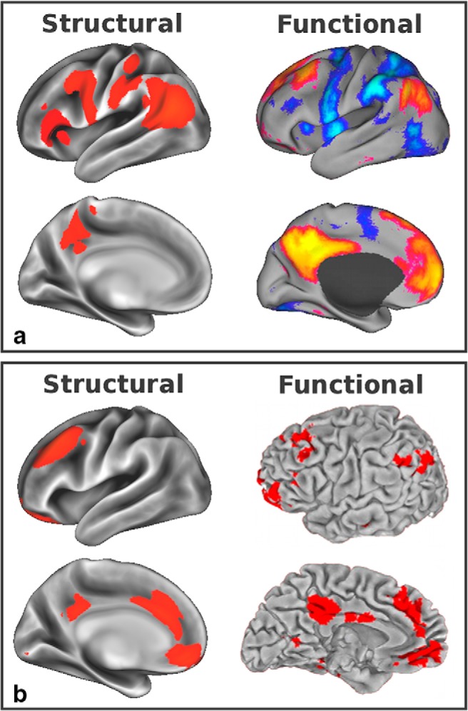
Two higher-level clusters involving DMN GMNs obtained using hierarchical clustering. a, Left, structural DMN 1 clustered with prefrontal regions and the intraparietal sulcus (|z| > 5), providing a structural underpinning for most of the functional DMN and its negatively correlated network (right, DMN in red-yellow and its anticorrelated network in blue-light blue, adapted from Fox et al., 2009). Two visual areas (middle temporal visual area/extrastriate body area and posterior intraparietal sulcus) are noticeably absent from this cluster as these regions clustered more strongly with other visual areas (an inherent limitation of hierarchical clustering in that each GMN can only appear once, in a single given cluster). b, DMN 2 was paired with executive (left, |z| > 5), the GMN resembling the executive control RSN, to create a cluster comparable to the limbic precuneus functional network (right, adapted from Margulies et al., 2009). The two structural clusters in a and b made up the entire DMN and its negatively correlated network (top right).

GMNs can be found in both half-split populations

We ran the linked ICA on our two subgroups of n = 242 subjects, each age matched to the original sample. The Bayesian model order selection retained 56 ICs in the first half-split and 54 ICs in the second (less than the 70 ICs requested). We identified from each run the ICs corresponding to our main GMN results (all with p < 10⁻³, although with a rougher spatial aspect due to the lower sample size; Table 4). Some of our GMNs were more readily identified in one of the subgroups (r > 0.5) or were found merged (e.g., visual 3 and 7, the two oculomotor networks). All of these identified ICs were significantly replicated (in terms of spatial correlation, p < 10⁻³) between the two half-split decompositions, except for visual 5, cerebellum 4, and two of the three frontal unilateral networks, the location of the latter two having been shown in the past to be particularly difficult to predict based on folding patterns (FreeSurfer cortical area) (Fischl et al., 2008).

Table 4.

Spatial correlations between the GMNs obtained in the full sample (N = 484) and in each of the two half-split samples (n = 242, matched for age to the original sample, all p < 10⁻³), as well as between the two half-split samples

GMNs	Group 1	Group 2	Group 1–Group 2
Visual 1	0.90	0.80	0.66
Cerebellum 3 (crus I versus crus II)	0.91	0.71	0.55
Auditory	0.80	0.79	0.53
Middle temporal sulcus	0.76	0.78	0.52
Executive	0.71	0.71	0.50
Other visual/motor (supplementary eye field)	0.71	0.71	0.50
Visual 6	0.71	0.68	0.64
Precentral versus inferior frontal gyrus	0.76	0.57	0.45
Visual 8	0.54	0.71	0.38
DMN 1	0.66	0.56	0.35
Sensorimotor 2 (lateral: sensory)	0.75	0.46	0.32
Frontoparietal (frontal 1) R	0.64	0.56	0.37
Cerebellum 1	0.58	0.59	0.64
Sensorimotor 1 (lateral: M1, premotor)	0.64	0.50	0.14
Visual 4	0.60	0.53	0.25
Visual 2	0.66	0.46	0.35
Other visual (parieto-occipital fissure)	0.53	0.59	0.35
Cerebellum 2	0.65	0.43	0.19
Frontoparietal (parietal) L	0.76	0.32	0.22
Frontoparietal (parietal) R	0.64	0.41	0.28
Olfactory (piriform)	0.32	0.72	0.23
Language	0.44	0.54	0.15
Sensorimotor 3 (medial)	0.40	0.56	0.32
Other visual (fusiform area: occipital)	0.32	0.59	0.23
Visual 3	0.55	0.35	0.39
Visual 7	0.55	0.35	0.39
Cerebellum 4	0.55	0.35	NS
DMN 2	0.29	0.61	0.16
Oculomotor 2 (posterior supplementary eye field)	0.49	0.34	0.46
Posterior superior temporal sulcus	0.55	0.25	0.35
Oculomotor 1 (frontal/premotor/cingulate eye field)	0.47	0.30	0.25
Frontoparietal (frontal) L	0.44	0.28	NS
Visual 5	0.40	0.31	NS
Frontoparietal (frontal 2) R	0.28	0.31	NS

The two half-split sets of ICs were identified by their similarities (spatial correlation in a whole-brain GM mask) to the full sample ICs and ranked according to their average across both subgroups. All spatial correlations between the two half-split sets of ICs were significant (p < 10⁻³), except for cerebellum 4, visual 5, and two of the three unilateral frontal networks.

NS, Not significant.

Discussion

In this study, we demonstrate that human structural architecture is functionally relevant across the entire brain. Modes of intersubject structural variability at a population level spatially correspond to functional organization that can be observed using both rest and task fMRI. Our analysis reveals fine-grained and highly functionally relevant anatomical networks, in particular in the cerebellum and visual cortex, and notably provides structural correspondence for the anterior DMN, the posterior DMN, and its anticorrelated functional network (Fox et al., 2009). As these intersubject brain structure networks emerge at a population level, this indicates that the trophic processes that render these distant parts of the brain functionally connected at the single-subject level may be developmental and evolutionary in nature.

Cerebellum

We identified four cerebellar GMNs with segregation that was functionally relevant: the lobules present together in each network are known to be functionally connected to the same regions of the cerebral cortex and subcortex (Sang et al., 2012). Crus I and II, the size of which is selectively expanded in humans (Balsters et al., 2010), notably emerged together in one distinct network (cerebellum 3). Consistent with the functional relevance of these segregations, hierarchical clustering yielded two higher-level clusters. The sensorimotor cluster (cerebellum 1 and 2), with a distinctive symmetry around the horizontal fissure, spatially matched the somatomotor map in the cerebellum obtained using functional connectivity of the cerebral, task-based location of movement (Buckner et al., 2011). Regions of the sensorimotor cluster show stronger motor activation relative to cognitive task (Stoodley et al., 2012), probably explaining the segregation observed between the cognitive (including cerebellum 3 and 4) and sensorimotor cerebellar clusters in our structural data.

Visual areas

We identified in the gray matter structure the same eight visual networks (visual 1–8) previously matched between rest and task fMRI (Smith et al., 2009), five of which actually better corresponded between structural and one functional dataset than between the two functional datasets (Table 3). Our hierarchical clustering approach demonstrated further the functional relevance of these subnetworks by creating, for instance, structural clusters underpinning perception of faces, places, and bodies or bringing together all cortical oculomotor control areas (magenta cluster; Fig. 9) (Amiez and Petrides, 2009).

DMN

The well documented functional segregation of the DMN into two anterior and posterior subnetworks was replicated by two structural modes of variation at the population level. This segregation not only corresponded to a natural division in the BrainMap fMRI database decomposed into higher dimensionality (Fig. 8) (Smith et al., 2009), but also to that of the limbic and cognitive connectivity patterns of the precuneus common to humans and macaques (whereby the more ventral region of the precuneus is functionally connected to the medial orbitofrontal regions) (Margulies et al., 2009). This segregation may also be related to distinct connectivity of the two DMN subnetworks with their respective anticorrelated network (Uddin et al., 2009). Consistent with this, the posterior DMN was strongly paired with a prefrontal GMN and in turn with a network centered around the anterior intraparietal sulcus; together, these three networks made up a structural equivalent for the functional posterior DMN and its negatively correlated functional network (Fox et al., 2009) (Fig. 10). This demonstrates that, whereas the two functionally anticorrelated networks represent a natural dichotomy between internally and externally directed cognitive processes (Spreng, 2012), they are structurally correlated at the population level. Furthermore, the anterior DMN paired with the executive GMN to create a cluster similar to the limbic precuneus functional network (Fig. 10) (Margulies et al., 2009), and this cluster itself paired with the right frontoparietal network (light green cluster; Fig. 9). The frontoparietal network is thought to mediate the DMN and its anticorrelated network (Vincent et al., 2008; Spreng, 2012). Our hierarchical clustering analysis thus shows that the structure underlying anterior DMN and (right) frontoparietal network on the one hand, posterior DMN and dorsal attention network on the other, varies together in size across the human population.

A few GMN maps showed a positive/negative pattern suggesting the expansion of one region at the expense of another at the population level. This pattern was in some cases found within the same brain region, pointing at known variability in the number of cortical folds in the healthy human brain, but in the majority of structural networks exhibiting this pattern, the positive and negative peaks were more distal. This was the case for crus I and crus II, which exhibited this positive/negative pattern within their structural network, as can be seen in Figure 6. Although the evolutionary reason for this competition between the two regions is unclear, it has been shown that crus I and II have in fact distinct function and relative size in humans (Balsters et al., 2010; Stoodley et al., 2012). Visual 3 provided another example, with positive contours broadly corresponding to V3 and V4 (Rottschy et al., 2007), but with negative nodes in the dorsal visual stream (centered exactly around the positive nodes of visual 7) in the posterior intraparietal sulcus. This might reinforce the idea of a dichotomy between dorsal and ventral V3 in humans that has been previously observed in the macaque (Newsome et al., 1986). A further way to witness competition between two regions of the brain was to look directly at negative correlations across the entire population. We found one correlation surviving Bonferroni correction between visual 1, centered around the calcarine fissure, and visual 6, the temporal FFA. This possibly hints at a development in humans of the latter, a cognitively highly specialized area, at the expense of the former, a primary visual area (Kanwisher and Yovel, 2006).

Previous studies have shown some degree of correspondence between functional connectivity and white matter connectivity, but have also found that strong functional connectivity can arise in the absence of direct white matter connectivity (Greicius et al., 2009; Honey et al., 2009; Alexander-Bloch et al., 2013). This possibly is in part due to limitation of the diffusion imaging technique itself in assessing long-range connections and in resolving crossing pathways (Jbabdi et al., 2015). For example, in the DMN, which has been arguably the most studied RSN for structural–functional connectivity correspondence, one such example can be seen in the medial orbitofrontal region. Although it is prominent in the functional DMN and in our gray matter structural connectivity network, it is absent from white matter structural connectivity analysis findings (Greicius et al., 2009; Honey et al., 2009). Another example can be seen in the prominence of the fusiform gyrus in our FLICA decomposition, something clearly reflected in the map showing the most shared gray matter regions across all structural GMNs (Fig. 3). The fusiform gyrus is, however, essentially absent from maps drawn from white matter connectivity (Hagmann et al., 2008; Gong et al., 2009; Nijhuis et al., 2013). Again, this likely is a consequence of the difficulty in reconstructing, both postmortem and in vivo, the white matter tracts connecting this specific gray matter region, mainly the inferior longitudinal fasciculus and the inferior frontooccipital fasciculus (Martino et al., 2010; Latini et al., 2017; Panesar et al., 2018). Conversely, one clear limitation of deriving structural networks from gray matter covariance, as opposed to white matter tractograms, is that these can only be estimated at the population level. However, our fine-grained, functionally meaningful results underline the benefit of looking at “connectivity” information obtained from simple, yet powerful T1-weighted imaging to efficiently capture covariations between far- or indirectly connected regions. Interestingly, those structural networks that can be formed at the population level seem to also partially overlap with the patterns of regions maturing together at the subject level (Geng et al., 2017; Khundrakpam et al., 2019).

Our multimodal approach also revealed that, similar to what is seen at the whole-brain level (Winkler et al., 2010), most of the gray matter volume networks colocalized with variation in cortical area and, importantly, that age and intracranial volume bore no effect on the results (after overall scaling was removed in the registration stage). As none of these GMNs was associated with intracranial volume (with the exception of cerebellum 1 and 4), this further reinforces the idea that cranial volume is not a determinant factor in the formation of cortical foldings in humans (Toro and Burnod, 2005; Bayly et al., 2014). The colocalization of our GMNs with variation in cortical area suggests that neurotrophic events occur during development, and possibly evolution, to dictate that the size and particularly the folding pattern of distant brain regions should vary together across subjects. Such trophic events, which might be reinforced by experience related plasticity (Evans, 2013), are likely to be (epi)genetically guided (Fjell et al., 2015; Toro et al., 2015) and be growth driven or due to axonal tension (Bayly et al., 2014), although there is currently no clear understanding of the cellular and molecular mechanisms underlying the emergence of such structural covariance networks (Alexander-Bloch et al., 2013). There are still some opposing views on a “concerted” or “mosaic” evolution of the brain, i.e., whether evolutionary changes in the size of one part of the brain can (“concerted”) or cannot (“mosaic”) co-occur with changes in all other parts (Finlay and Darlington, 1995; Yopak et al., 2010; Hager et al., 2012). What seems to emerge increasingly is conciliatory; however, although there is evidence for a mosaic evolution of the brain with certain brain regions evolving independently from others, functionally related parts of the brain seem to vary together across species (Barton and Harvey, 2000; Moore and DeVoogd, 2017). Our cortical folding results not only suggest this is something that might also be reflected in human development, but also support the concept that there might exist a close relationship between convolutional anatomy and the organization of cortical function (Bayly et al., 2014).

References

- Alexander-Bloch A, Giedd JN, Bullmore E (2013) Imaging structural covariance between human brain regions. Nat Rev Neurosci 14:322–336. 10.1038/nrn3465 [DOI] [PMC free article] [PubMed] [Google Scholar]
- Amiez C, Petrides M (2009) Anatomical organization of the eye fields in the human and non-human primate frontal cortex. Prog Neurobiol 89:220–230. 10.1016/j.pneurobio.2009.07.010 [DOI] [PubMed] [Google Scholar]
- Amunts K, Schleicher A, Bürgel U, Mohlberg H, Uylings HB, Zilles K (1999) Broca's region revisited: cytoarchitecture and intersubject variability. J Comp Neurol 412:319–341. [DOI] [PubMed] [Google Scholar]
- Ashburner J, Friston KJ (2000) Voxel-based morphometry–the methods. Neuroimage 11:805–821. 10.1006/nimg.2000.0582 [DOI] [PubMed] [Google Scholar]
- Balsters JH, Cussans E, Diedrichsen J, Phillips KA, Preuss TM, Rilling JK, Ramnani N (2010) Evolution of the cerebellar cortex: the selective expansion of prefrontal-projecting cerebellar lobules. Neuroimage 49:2045–2052. 10.1016/j.neuroimage.2009.10.045 [DOI] [PMC free article] [PubMed] [Google Scholar]
- Barton RA, Harvey PH (2000) Mosaic evolution of brain structure in mammals. Nature 405:1055–1058. 10.1038/35016580 [DOI] [PubMed] [Google Scholar]
- Bayly PV, Taber LA, Kroenke CD (2014) Mechanical forces in cerebral cortical folding: a review of measurements and models. J Mech Behav Biomed Mater 29:568–581. 10.1016/j.jmbbm.2013.02.018 [DOI] [PMC free article] [PubMed] [Google Scholar]
- Beckmann CF, DeLuca M, Devlin JT, Smith SM (2005) Investigations into resting-state connectivity using independent component analysis. Philos Trans R Soc Lond B Biol Sci 360:1001–1013. 10.1098/rstb.2005.1634 [DOI] [PMC free article] [PubMed] [Google Scholar]
- Buckner RL, Krienen FM, Castellanos A, Diaz JC, Yeo BT (2011) The organization of the human cerebellum estimated by intrinsic functional connectivity. J Neurophysiol 106:2322–2345. 10.1152/jn.00339.2011 [DOI] [PMC free article] [PubMed] [Google Scholar]
- Caspers S, Geyer S, Schleicher A, Mohlberg H, Amunts K, Zilles K (2006) The human inferior parietal cortex: cytoarchitectonic parcellation and interindividual variability. Neuroimage 33:430–448. 10.1016/j.neuroimage.2006.06.054 [DOI] [PubMed] [Google Scholar]
- Cauda F, Nani A, Manuello J, Premi E, Palermo S, Tatu K, Duca S, Fox PT, Costa T (2018) Brain structural alterations are distributed following functional, anatomic and genetic connectivity. Brain 141:3211–3232. 10.1093/brain/awy252 [DOI] [PMC free article] [PubMed] [Google Scholar]
- Chen ZJ, He Y, Rosa-Neto P, Germann J, Evans AC (2008) Revealing modular architecture of human brain structural networks by using cortical thickness from MRI. Cereb Cortex 18:2374–2381. 10.1093/cercor/bhn003 [DOI] [PMC free article] [PubMed] [Google Scholar]
- Dale AM, Fischl B, Sereno MI (1999) Cortical surface-based analysis. I. Segmentation and surface reconstruction. Neuroimage 9:179–194. 10.1006/nimg.1998.0395 [DOI] [PubMed] [Google Scholar]
- Diedrichsen J, Balsters JH, Flavell J, Cussans E, Ramnani N (2009) A probabilistic MR atlas of the human cerebellum. Neuroimage 46:39–46. 10.1016/j.neuroimage.2009.01.045 [DOI] [PubMed] [Google Scholar]
- Doan NT, Engvig A, Zaske K, Persson K, Lund MJ, Kaufmann T, Cordova-Palomera A, Alnæs D, Moberget T, Brækhus A, Barca ML, Nordvik JE, Engedal K, Agartz I, Selbæk G, Andreassen OA, Westlye LT, Westlye LT (2017a) Distinguishing early and late brain aging from the Alzheimer's disease spectrum: consistent morphological patterns across independent samples. Neuroimage 158:282–295. 10.1016/j.neuroimage.2017.06.070 [DOI] [PubMed] [Google Scholar]
- Doan NT, Kaufmann T, Bettella F, Jørgensen KN, Brandt CL, Moberget T, Alnæs D, Douaud G, Duff E, Djurovic S, Melle I, Ueland T, Agartz I, Andreassen OA, Westlye LT (2017b) Distinct multivariate brain morphological patterns and their added predictive value with cognitive and polygenic risk scores in mental disorders. Neuroimage Clin 15:719–731. 10.1016/j.nicl.2017.06.014 [DOI] [PMC free article] [PubMed] [Google Scholar]
- Douaud G, Smith S, Jenkinson M, Behrens T, Johansen-Berg H, Vickers J, James S, Voets N, Watkins K, Matthews PM, James A (2007) Anatomically related grey and white matter abnormalities in adolescent-onset schizophrenia. Brain 130:2375–2386. 10.1093/brain/awm184 [DOI] [PubMed] [Google Scholar]
- Douaud G, Groves AR, Tamnes CK, Westlye LT, Duff EP, Engvig A, Walhovd KB, James A, Gass A, Monsch AU, Matthews PM, Fjell AM, Smith SM, Johansen-Berg H (2014) A common brain network links development, aging, and vulnerability to disease. Proc Natl Acad Sci U S A 111:17648–17653. 10.1073/pnas.1410378111 [DOI] [PMC free article] [PubMed] [Google Scholar]
- Eickhoff SB, Stephan KE, Mohlberg H, Grefkes C, Fink GR, Amunts K, Zilles K (2005) A new SPM toolbox for combining probabilistic cytoarchitectonic maps and functional imaging data. Neuroimage 25:1325–1335. 10.1016/j.neuroimage.2004.12.034 [DOI] [PubMed] [Google Scholar]
- Evans AC. (2013) Networks of anatomical covariance. Neuroimage 80:489–504. 10.1016/j.neuroimage.2013.05.054 [DOI] [PubMed] [Google Scholar]
- Finlay BL, Darlington RB (1995) Linked regularities in the development and evolution of mammalian brains. Science 268:1578–1584. 10.1126/science.7777856 [DOI] [PubMed] [Google Scholar]
- Finn ES, Shen X, Scheinost D, Rosenberg MD, Huang J, Chun MM, Papademetris X, Constable RT (2015) Functional connectome fingerprinting: identifying individuals using patterns of brain connectivity. Nat Neurosci 18:1664–1671. 10.1038/nn.4135 [DOI] [PMC free article] [PubMed] [Google Scholar]
- Fischl B, Dale AM (2000) Measuring the thickness of the human cerebral cortex from magnetic resonance images. Proc Natl Acad Sci U S A 97:11050–11055. 10.1073/pnas.200033797 [DOI] [PMC free article] [PubMed] [Google Scholar]
- Fischl B, Sereno MI, Dale AM (1999) Cortical surface-based analysis. II: inflation, flattening, and a surface-based coordinate system. Neuroimage 9:195–207. 10.1006/nimg.1998.0396 [DOI] [PubMed] [Google Scholar]
- Fischl B, Salat DH, Busa E, Albert M, Dieterich M, Haselgrove C, van der Kouwe A, Killiany R, Kennedy D, Klaveness S, Montillo A, Makris N, Rosen B, Dale AM (2002) Whole brain segmentation: automated labeling of neuroanatomical structures in the human brain. Neuron 33:341–355. 10.1016/S0896-6273(02)00569-X [DOI] [PubMed] [Google Scholar]
- Fischl B, Rajendran N, Busa E, Augustinack J, Hinds O, Yeo BT, Mohlberg H, Amunts K, Zilles K (2008) Cortical folding patterns and predicting cytoarchitecture. Cereb Cortex 18:1973–1980. 10.1093/cercor/bhm225 [DOI] [PMC free article] [PubMed] [Google Scholar]
- Fjell AM, Grydeland H, Krogsrud SK, Amlien I, Rohani DA, Ferschmann L, Storsve AB, Tamnes CK, Sala-Llonch R, Due-Tønnessen P, Bjørnerud A, Sølsnes AE, Håberg AK, Skranes J, Bartsch H, Chen CH, Thompson WK, Panizzon MS, Kremen WS, Dale AM, Walhovd KB (2015) Development and aging of cortical thickness correspond to genetic organization patterns. Proc Natl Acad Sci U S A 112:15462–15467. 10.1073/pnas.1508831112 [DOI] [PMC free article] [PubMed] [Google Scholar]
- Fox MD, Zhang D, Snyder AZ, Raichle ME (2009) The global signal and observed anticorrelated resting state brain networks. J Neurophysiol 101:3270–3283. 10.1152/jn.90777.2008 [DOI] [PMC free article] [PubMed] [Google Scholar]
- Fox PT, Lancaster JL (2002) Opinion: mapping context and content: the BrainMap model. Nat Rev Neurosci 3:319–321. 10.1038/nrn789 [DOI] [PubMed] [Google Scholar]
- Francx W, Llera A, Mennes M, Zwiers MP, Faraone SV, Oosterlaan J, Heslenfeld D, Hoekstra PJ, Hartman CA, Franke B, Buitelaar JK, Beckmann CF (2016) Integrated analysis of gray and white matter alterations in attention-deficit/hyperactivity disorder. Neuroimage Clin 11:357–367. 10.1016/j.nicl.2016.03.005 [DOI] [PMC free article] [PubMed] [Google Scholar]
- Geng X, Li G, Lu Z, Gao W, Wang L, Shen D, Zhu H, Gilmore JH (2017) Structural and maturational covariance in early childhood brain development. Cereb Cortex 27:1795–1807. 10.1093/cercor/bhw022 [DOI] [PMC free article] [PubMed] [Google Scholar]
- Geyer S, Ledberg A, Schleicher A, Kinomura S, Schormann T, Burgel U, Klingberg T, Larsson J, Zilles K, Roland PE (1996) Two different areas within the primary motor cortex of man. Nature 382:805–807. 10.1038/382805a0 [DOI] [PubMed] [Google Scholar]
- Geyer S, Matelli M, Luppino G, Zilles K (2000) Functional neuroanatomy of the primate isocortical motor system. Anat Embryol (Berl) 202:443–474. [DOI] [PubMed] [Google Scholar]
- Gong G, He Y, Concha L, Lebel C, Gross DW, Evans AC, Beaulieu C (2009) Mapping anatomical connectivity patterns of human cerebral cortex using in vivo diffusion tensor imaging tractography. Cereb Cortex 19:524–536. 10.1093/cercor/bhn102 [DOI] [PMC free article] [PubMed] [Google Scholar]
- Goodkind M, Eickhoff SB, Oathes DJ, Jiang Y, Chang A, Jones-Hagata LB, Ortega BN, Zaiko YV, Roach EL, Korgaonkar MS, Grieve SM, Galatzer-Levy I, Fox PT, Etkin A (2015) Identification of a common neurobiological substrate for mental illness. JAMA Psychiatry 72:305–315. 10.1001/jamapsychiatry.2014.2206 [DOI] [PMC free article] [PubMed] [Google Scholar]
- Greicius MD, Supekar K, Menon V, Dougherty RF (2009) Resting-state functional connectivity reflects structural connectivity in the default mode network. Cereb Cortex 19:72–78. 10.1093/cercor/bhn059 [DOI] [PMC free article] [PubMed] [Google Scholar]
- Groves AR, Beckmann CF, Smith SM, Woolrich MW (2011) Linked independent component analysis for multimodal data fusion. Neuroimage 54:2198–2217. 10.1016/j.neuroimage.2010.09.073 [DOI] [PubMed] [Google Scholar]
- Groves AR, Smith SM, Fjell AM, Tamnes CK, Walhovd KB, Douaud G, Woolrich MW, Westlye LT (2012) Benefits of multi-modal fusion analysis on a large-scale dataset: life-span patterns of inter-subject variability in cortical morphometry and white matter microstructure. Neuroimage 63:365–380. 10.1016/j.neuroimage.2012.06.038 [DOI] [PubMed] [Google Scholar]
- Grydeland H, Vértes PE, Váša F, Romero-Garcia R, Whitaker K, Alexander-Bloch AF, Bjørnerud A, Patel AX, Sederevicius D, Tamnes CK, Westlye LT, White SR, Walhovd KB, Fjell AM, Bullmore ET (2019) Waves of maturation and senescence in micro-structural MRI markers of human cortical myelination over the lifespan. Cereb Cortex 29:1369–1381. 10.1093/cercor/bhy330 [DOI] [PMC free article] [PubMed] [Google Scholar]
- Hager R, Lu L, Rosen GD, Williams RW (2012) Genetic architecture supports mosaic brain evolution and independent brain-body size regulation. Nat Commun 3:1079. 10.1038/ncomms2086 [DOI] [PMC free article] [PubMed] [Google Scholar]
- Hagmann P, Cammoun L, Gigandet X, Meuli R, Honey CJ, Wedeen VJ, Sporns O (2008) Mapping the structural core of human cerebral cortex. PLoS Biol 6:e159. 10.1371/journal.pbio.0060159 [DOI] [PMC free article] [PubMed] [Google Scholar]
- Honey CJ, Sporns O, Cammoun L, Gigandet X, Thiran JP, Meuli R, Hagmann P (2009) Predicting human resting-state functional connectivity from structural connectivity. Proc Natl Acad Sci U S A 106:2035–2040. 10.1073/pnas.0811168106 [DOI] [PMC free article] [PubMed] [Google Scholar]
- Jalbrzikowski M, Jonas R, Senturk D, Patel A, Chow C, Green MF, Bearden CE (2013) Structural abnormalities in cortical volume, thickness, and surface area in 22q11.2 microdeletion syndrome: relationship with psychotic symptoms. Neuroimage Clin 3:405–415. 10.1016/j.nicl.2013.09.013 [DOI] [PMC free article] [PubMed] [Google Scholar]
- Jbabdi S, Sotiropoulos SN, Haber SN, Van Essen DC, Behrens TE (2015) Measuring macroscopic brain connections in vivo. Nat Neurosci 18:1546–1555. 10.1038/nn.4134 [DOI] [PubMed] [Google Scholar]
- Kanwisher N, Dilks DD (2013) The functional organization of the ventral visual pathway in humans. In: The new visual neurosciences (Chalupa LM, Werner JS, eds), pp 733–746. Cambridge: MIT. [Google Scholar]
- Kanwisher N, Yovel G (2006) The fusiform face area: a cortical region specialized for the perception of faces. Philos Trans R Soc Lond B Biol Sci 361:2109–2128. 10.1098/rstb.2006.1934 [DOI] [PMC free article] [PubMed] [Google Scholar]
- Khundrakpam BS, Lewis JD, Jeon S, Kostopoulos P, Itturia Medina Y, Chouinard-Decorte F, Evans AC (2019) Exploring individual brain variability during development based on patterns of maturational coupling of cortical thickness: a longitudinal MRI study. Cereb Cortex 29:178–188. 10.1093/cercor/bhx317 [DOI] [PubMed] [Google Scholar]
- Kirk RE. (1996) Practical significance: a concept whose time has come. Educ Psychol Meas 56:746–759. 10.1177/0013164496056005002 [DOI] [Google Scholar]
- Latini F, Mårtensson J, Larsson EM, Fredrikson M, Åhs F, Hjortberg M, Aldskogius H, Ryttlefors M (2017) Segmentation of the inferior longitudinal fasciculus in the human brain: a white matter dissection and diffusion tensor tractography study. Brain Res 1675:102–115. 10.1016/j.brainres.2017.09.005 [DOI] [PubMed] [Google Scholar]
- Leech R, Kamourieh S, Beckmann CF, Sharp DJ (2011) Fractionating the default mode network: distinct contributions of the ventral and dorsal posterior cingulate cortex to cognitive control. J Neurosci 31:3217–3224. 10.1523/JNEUROSCI.5626-10.2011 [DOI] [PMC free article] [PubMed] [Google Scholar]
- Margulies DS, Vincent JL, Kelly C, Lohmann G, Uddin LQ, Biswal BB, Villringer A, Castellanos FX, Milham MP, Petrides M (2009) Precuneus shares intrinsic functional architecture in humans and monkeys. Proc Natl Acad Sci U S A 106:20069–20074. 10.1073/pnas.0905314106 [DOI] [PMC free article] [PubMed] [Google Scholar]
- Marquand AF, Wolfers T, Mennes M, Buitelaar J, Beckmann CF (2016) Beyond lumping and splitting: a review of computational approaches for stratifying psychiatric disorders. Biol Psychiatry Cogn Neurosci Neuroimaging 1:433–447. 10.1016/j.bpsc.2016.04.002 [DOI] [PMC free article] [PubMed] [Google Scholar]
- Martino J, Brogna C, Robles SG, Vergani F, Duffau H (2010) Anatomic dissection of the inferior fronto-occipital fasciculus revisited in the lights of brain stimulation data. Cortex 46:691–699. 10.1016/j.cortex.2009.07.015 [DOI] [PubMed] [Google Scholar]
- Mesulam MM. (1998) From sensation to cognition. Brain 121:1013–1052. 10.1093/brain/121.6.1013 [DOI] [PubMed] [Google Scholar]
- Moore JM, DeVoogd TJ (2017) Concerted and mosaic evolution of functional modules in songbird brains. Proc Biol Sci 284:20170469. 10.1098/rspb.2017.0469 [DOI] [PMC free article] [PubMed] [Google Scholar]
- Newsome WT, Maunsell JH, Van Essen DC (1986) Ventral posterior visual area of the macaque: visual topography and areal boundaries. J Comp Neurol 252:139–153. 10.1002/cne.902520202 [DOI] [PubMed] [Google Scholar]
- Nijhuis EH, van Cappellen van Walsum AM, Norris DG (2013) Topographic hub maps of the human structural neocortical network. PLoS One 8:e65511. 10.1371/journal.pone.0065511 [DOI] [PMC free article] [PubMed] [Google Scholar]
- Panesar SS, Yeh FC, Jacquesson T, Hula W, Fernandez-Miranda JC (2018) A quantitative tractography study into the connectivity, segmentation and laterality of the human inferior longitudinal fasciculus. Front Neuroanat 12:47. 10.3389/fnana.2018.00047 [DOI] [PMC free article] [PubMed] [Google Scholar]
- Raj A, Kuceyeski A, Weiner M (2012) A network diffusion model of disease progression in dementia. Neuron 73:1204–1215. 10.1016/j.neuron.2011.12.040 [DOI] [PMC free article] [PubMed] [Google Scholar]
- Rottschy C, Eickhoff SB, Schleicher A, Mohlberg H, Kujovic M, Zilles K, Amunts K (2007) Ventral visual cortex in humans: cytoarchitectonic mapping of two extrastriate areas. Hum Brain Mapp 28:1045–1059. 10.1002/hbm.20348 [DOI] [PMC free article] [PubMed] [Google Scholar]
- Sang L, Qin W, Liu Y, Han W, Zhang Y, Jiang T, Yu C (2012) Resting-state functional connectivity of the vermal and hemispheric subregions of the cerebellum with both the cerebral cortical networks and subcortical structures. Neuroimage 61:1213–1225. 10.1016/j.neuroimage.2012.04.011 [DOI] [PubMed] [Google Scholar]
- Schmahmann JD. (2000) MRI atlas of the human cerebellum. San Diego: Academic. [Google Scholar]
- Seeley WW, Crawford RK, Zhou J, Miller BL, Greicius MD (2009) Neurodegenerative diseases target large-scale human brain networks. Neuron 62:42–52. 10.1016/j.neuron.2009.03.024 [DOI] [PMC free article] [PubMed] [Google Scholar]
- Segall JM, Allen EA, Jung RE, Erhardt EB, Arja SK, Kiehl K, Calhoun VD (2012) Correspondence between structure and function in the human brain at rest. Front Neuroinform 6:10. 10.3389/fninf.2012.00010 [DOI] [PMC free article] [PubMed] [Google Scholar]
- Sharika KM, Neggers SF, Gutteling TP, Van der Stigchel S, Dijkerman HC, Murthy A (2013) Proactive control of sequential saccades in the human supplementary eye field. Proc Natl Acad Sci U S A 110:E1311–E1320. 10.1073/pnas.1210492110 [DOI] [PMC free article] [PubMed] [Google Scholar]
- Smith SM, Jenkinson M, Woolrich MW, Beckmann CF, Behrens TE, Johansen-Berg H, Bannister PR, De Luca M, Drobnjak I, Flitney DE, Niazy RK, Saunders J, Vickers J, Zhang Y, De Stefano N, Brady JM, Matthews PM (2004) Advances in functional and structural MR image analysis and implementation as FSL. Neuroimage 23:S208–S219. 10.1016/j.neuroimage.2004.07.051 [DOI] [PubMed] [Google Scholar]
- Smith SM, Fox PT, Miller KL, Glahn DC, Fox PM, Mackay CE, Filippini N, Watkins KE, Toro R, Laird AR, Beckmann CF (2009) Correspondence of the brain's functional architecture during activation and rest. Proc Natl Acad Sci U S A 106:13040–13045. 10.1073/pnas.0905267106 [DOI] [PMC free article] [PubMed] [Google Scholar]
- Sporns O. (2014) Contributions and challenges for network models in cognitive neuroscience. Nat Neurosci 17:652–660. 10.1038/nn.3690 [DOI] [PubMed] [Google Scholar]
- Spreng RN. (2012) The fallacy of a “task-negative” network. Front Psychol 3:145. 10.3389/fpsyg.2012.00145 [DOI] [PMC free article] [PubMed] [Google Scholar]
- Stephen JM, Coffman BA, Jung RE, Bustillo JR, Aine CJ, Calhoun VD (2013) Using joint ICA to link function and structure using MEG and DTI in schizophrenia. Neuroimage 83:418–430. 10.1016/j.neuroimage.2013.06.038 [DOI] [PMC free article] [PubMed] [Google Scholar]
- Stoodley CJ, Valera EM, Schmahmann JD (2012) Functional topography of the cerebellum for motor and cognitive tasks: an fMRI study. Neuroimage 59:1560–1570. 10.1016/j.neuroimage.2011.08.065 [DOI] [PMC free article] [PubMed] [Google Scholar]
- Storsve AB, Fjell AM, Tamnes CK, Westlye LT, Overbye K, Aasland HW, Walhovd KB (2014) Differential longitudinal changes in cortical thickness, surface area and volume across the adult life span: regions of accelerating and decelerating change. J Neurosci 34:8488–8498. 10.1523/JNEUROSCI.0391-14.2014 [DOI] [PMC free article] [PubMed] [Google Scholar]
- Sui J, Pearlson G, Caprihan A, Adali T, Kiehl KA, Liu J, Yamamoto J, Calhoun VD (2011) Discriminating schizophrenia and bipolar disorder by fusing fMRI and DTI in a multimodal CCA+ joint ICA model. Neuroimage 57:839–855. 10.1016/j.neuroimage.2011.05.055 [DOI] [PMC free article] [PubMed] [Google Scholar]
- Toro R, Burnod Y (2005) A morphogenetic model for the development of cortical convolutions. Cereb Cortex 15:1900–1913. 10.1093/cercor/bhi068 [DOI] [PubMed] [Google Scholar]
- Toro R, Poline JB, Huguet G, Loth E, Frouin V, Banaschewski T, Barker GJ, Bokde A, Büchel C, Carvalho FM, Conrod P, Fauth-Bühler M, Flor H, Gallinat J, Garavan H, Gowland P, Heinz A, Ittermann B, Lawrence C, Lemaître H, et al. (2015) Genomic architecture of human neuroanatomical diversity. Mol Psychiatry 20:1011–1016. 10.1038/mp.2014.99 [DOI] [PubMed] [Google Scholar]
- Uddin LQ, Kelly AM, Biswal BB, Castellanos FX, Milham MP (2009) Functional connectivity of default mode network components: correlation, anticorrelation, and causality. Hum Brain Mapp 30:625–637. 10.1002/hbm.20531 [DOI] [PMC free article] [PubMed] [Google Scholar]
- Vincent JL, Kahn I, Snyder AZ, Raichle ME, Buckner RL (2008) Evidence for a frontoparietal control system revealed by intrinsic functional connectivity. J Neurophysiol 100:3328–3342. 10.1152/jn.90355.2008 [DOI] [PMC free article] [PubMed] [Google Scholar]
- Voets NL, Hough MG, Douaud G, Matthews PM, James A, Winmill L, Webster P, Smith S (2008) Evidence for abnormalities of cortical development in adolescent-onset schizophrenia. Neuroimage 43:665–675. 10.1016/j.neuroimage.2008.08.013 [DOI] [PubMed] [Google Scholar]
- Winkler AM, Kochunov P, Blangero J, Almasy L, Zilles K, Fox PT, Duggirala R, Glahn DC (2010) Cortical thickness or grey matter volume? The importance of selecting the phenotype for imaging genetics studies. Neuroimage 53:1135–1146. 10.1016/j.neuroimage.2009.12.028 [DOI] [PMC free article] [PubMed] [Google Scholar]
- Winkler AM, Greve DN, Bjuland KJ, Nichols TE, Sabuncu MR, Håberg AK, Skranes J, Rimol LM (2018) Joint analysis of cortical area and thickness as a replacement for the analysis of the volume of the cerebral cortex. Cereb Cortex 28:738–749. 10.1093/cercor/bhx308 [DOI] [PMC free article] [PubMed] [Google Scholar]
- Yopak KE, Lisney TJ, Darlington RB, Collin SP, Montgomery JC, Finlay BL (2010) A conserved pattern of brain scaling from sharks to primates. Proc Natl Acad Sci U S A 107:12946–12951. 10.1073/pnas.1002195107 [DOI] [PMC free article] [PubMed] [Google Scholar]
- Zeighami Y, Ulla M, Iturria-Medina Y, Dadar M, Zhang Y, Larcher KM, Fonov V, Evans AC, Collins DL, Dagher A (2015) Network structure of brain atrophy in de novo Parkinson's disease. Elife 4: e08440. 10.7554/eLife.08440 [DOI] [PMC free article] [PubMed] [Google Scholar]