Abstract
Extended reduced graphs provide summary representations of chemical structures using pharmacophore-type node descriptions to encode the relevant molecular properties. Commonly used similarity measures using reduced graphs convert these graphs into 2D vectors like fingerprints, before chemical comparisons are made. This study investigates the effectiveness of a graph-only driven molecular comparison by using extended reduced graphs along with graph edit distance methods for molecular similarity calculation as a tool for ligand-based virtual screening applications, which estimate the bioactivity of a chemical on the basis of the bioactivity of similar compounds. The results proved to be very stable and the graph editing distance method performed better than other methods previously used on reduced graphs. This is exemplified with six publicly available data sets: DUD-E, MUV, GLL&GDD, CAPST, NRLiSt BDB, and ULS-UDS. The screening and statistical tools available on the ligand-based virtual screening benchmarking platform and the RDKit were also used. In the experiments, our method performed better than other molecular similarity methods which use array representations in most cases. Overall, it is shown that extended reduced graphs along with graph edit distance is a combination of methods that has numerous applications and can identify bioactivity similarities in a structurally diverse group of molecules.
Introduction
With the massive increase in data on chemical compounds and their activities thanks to the development of high-throughput screening techniques, there is an increasing demand for computational tools to improve the drug synthesis and test cycle. These tools are crucial if activity data are to be analyzed and new models created to be used in virtual screening techniques.1
Virtual screening, that is to say, the use of computational techniques to search and filter chemical databases,2,3 has become a common step in the drug discovery process. Virtual screening has two main categories: structure-based (SBVS)4 and ligand-based virtual screening (LBVS).5 LVBS uses information about the known activity of some molecules to predict the unknown activity of new molecules. The main LBVS approaches are pharmacophore mapping,6 shape-based similarity,7 fingerprint similarity, and various machine learning methods.8 The concept of molecular similarity is frequently used in the context of LBVS, and the measure of molecular similarity used is an important feature that determines the success or not of a virtual screening method.
Molecular similarity methods are commonly used to select good candidates in the drug discovery industry because it is assumed that structurally similar molecules are likely to have similar properties.9 These methods are included in applications such as molecular screening, similarity searching, or molecular clustering.10−14
Molecular similarity searching usually requires the descriptors representing the molecules to be defined and a method by which the level of similarity among the molecules can be quantified. Various types of descriptors have been used,3,15,16 which can be catalogued as one-dimensional (1D), two-dimensional (2D), or three-dimensional (3D) depending on the molecular representations used to calculate them.17 Some descriptors include general molecular properties (1D descriptors) such as size, molecular weight, logP, dipole moment, BCUT parameters, etc.18−21 while others create array representations of the molecules by simplifying the atomic information in them such as 2D fingerprints.22−25 There are also 3D descriptors that simplify the 3D information such as molecular volume.26,27 Additionally, some methods represent compounds as trees28 and graphs.29,30 Some of these methods represent the compounds using reduced graphs,31−34 which group atomic substructures together on the basis of related features such as ring systems, hydrogen-bonding, pharmacophoric features or other rules. Moreover, extended reduced graphs (ErG)34 is an extension of the reduced graphs described by Gillet et al.,33 and makes specific modifications to better describe the pharmacophoric properties, size, and shape of the molecules.
Two similarity measures have been defined to compare reduced graphs. They map the reduced graphs into a 2D fingerprint33−35 or into sets of shortest paths.36 Research is ongoing into new methods for measuring molecular similarity, mainly because of the difficulty to describe the relationship between the complex chemical space and its biological activity.
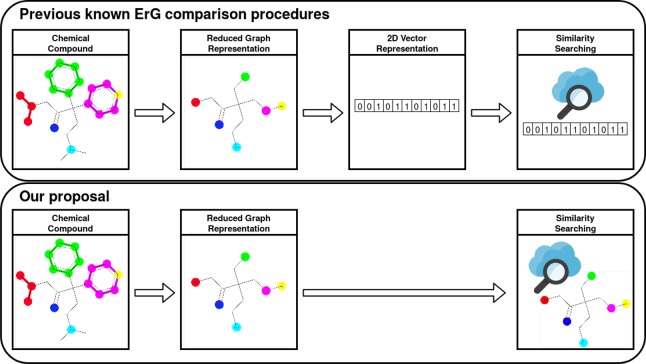
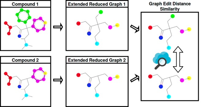
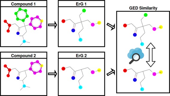
ErGs have proved to be a very useful tool for virtual screening,34 particularly because they can work as an abstraction from the complex physico-atomic world, and enable us to have direct experience with the pharmacophoric chemical information inside the molecular structures. The main goal of this study is to implement a graph-only driven molecular comparison methodology, without the array representations. The comparison is made directly on graphs and there is no need to perform any transformation from graphs into 2D vectors (Figure 1). In our new model, graph edit distance (GED)37−40 has been used as similarity measurement between molecular structures based on ErG. GED computes a cost distance between two graphs, that is to say, the minimum modifications required to transform one graph into another. Each modification can be one of six operations: insertion, deletion, and substitution for both nodes and edges in the graph.
Figure 1.
Molecular comparison flowcharts. Difference between traditional ErG methods and our proposal.
This paper is organized as follows. First, materials and methods are presented and explained in detail. Second, computational results are shown. And third, a final discussion concludes the paper.
Materials and Methods
Data Sets
Six publicly available data sets were used in this study. They are ULS and UDS,41 GDD and GLL,42 DUD Release 243 (DUD-E), NRLiSt BDB,44 MUV,45 and a data set from Comparative Analysis of Pharmacophore Screening Tools46 (CAPST). All these data sets were normalized in a format ready to use by the LBVS benchmarking platform developed by Skoda and Hoksza.47 This platform is similar in concept to another benchmarking platform developed by Riniker and Landrum and has extended some of its features.48 The data sets formatted to be used with this platform consist of several selections of active and inactive molecules grouped according to different targets. Each selection is separated into test and train sets so that it can be used for machine learning applications. Each selection is presented as a predefined random-built collection of constant splits so that the results are fully reproducible, and the negative effects of randomness should be mitigated by using multiple splits for each selection. These selections are also catalogued according to their level of difficulty, which was estimated by analyzing performance trends for several commonly used LBVS methods in terms of the resulting Area Under the Receiver Operating Characteristic curve (AUC)49 value.
Molecular Representation
Reduced graphs are smaller abstractions of the original chemical graph in whichthe main information is condensed in feature nodes to give summary representations of the chemical structures. Depending on the features they summarize or the use to which they are put, different versions of reduced graphs can be used. In the case of virtual screening, the structure is reduced to localize features of structures that have the potential to interact with receptors while retaining the spatial distribution and topology among the features.
In this study, the reduction methodology used is the one described by Stiefl et al.,34 in which the main features are pharmacophore-type node descriptions. This method is called ErG, and as the authors point out, it can be described as a hybrid approach of reduced graphs33 and binding property pairs.50
In ErG, nodes can be one or a combination of the following features: hydrogen-bond donor, hydrogen-bond acceptor, positive charge, negative charge, hydrophobic group and aromatic ring system. Some featureless nodes also work as links to the relevant features. These can be carbon or noncarbon link nodes. One example of an ErG can be seen in Figure 2. The upper part of the figure shows an example molecule with the pharmacophoric substructures highlighted. The lower part of the figure shows the ErG obtained from the example molecule.
Figure 2.
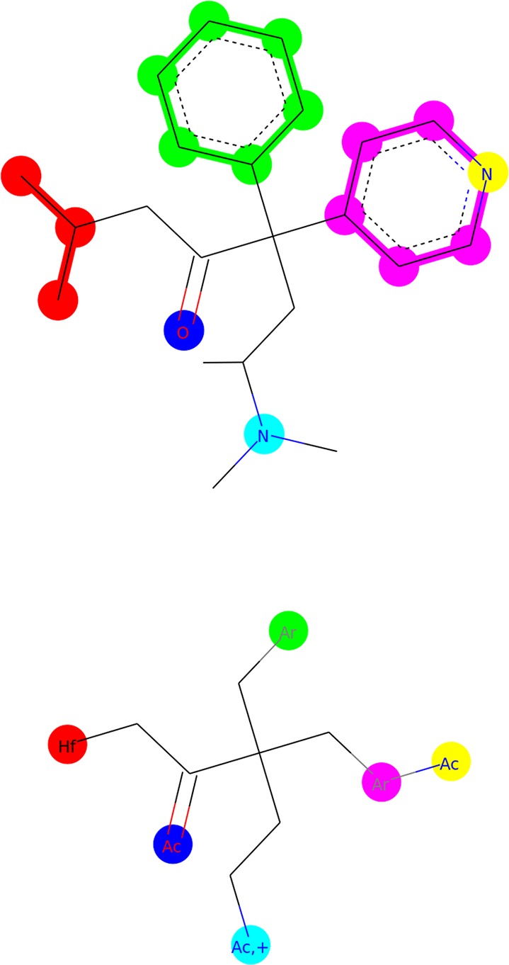
Example of molecule reduction using ErG. At the top there is the original molecule and at the bottom the ErG representation. Ac: H-bond acceptor; Hf: hydrophobic group; Ar: aromatic ring system; +: positive charge. Colors are used to show how different parts of the original structure are reduced to nodes in the ErG.
Molecular Comparison
Once the molecular structure has been represented as an ErG, the next step is to define a similarity procedure to measure how similar two molecules are by comparing their ErGs. In this paper, we summarize two reported methods and we present a new one: first method: fingerprint-based, used by the authors in the paper that reported ErGs for the first time;34 second method: string edit distance (SED)-based, presented by Harper et al.;36 third method: our new proposal, GED-based, which aims to compare ErGs directly with no intermediate representation. We shall now go on to describe these three methodologies in detail.
Fingerprint-Based
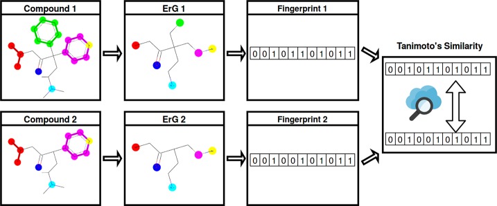
Generally speaking, fingerprint-based methods code the molecular structure in a vector array called a fingerprint (see Figure 3). Each bin denotes the presence or absence of a particular substructure. Then, the similarity between two molecules A and B is computed by comparing their fingerprints with a measure such as the Tanimoto similarity index (eq 1).
| 1 |
where A∩B stands for the intersection and A∪B is the union of the sets of bins in the fingerprints A and B. Furthermore, |A| and |B| represent the number of nonempty bins in the sets A and B. The resulting value goes from 0 to 1, with 1 representing the highest degree of similarity.
Figure 3.
Fingerprint-based method flowchart.
In the specific context of ErGs, the fingerprint descriptor used by Stiefl et al. is based on the method used by Kearsley et al. for their binding property pairs,50 which, in turn, is an extension of the atom pairs described by Carhart et al.51
Atom pairs are built using substructures of the form
where (distance) represents the distance between atom i and atom j along the shortest path. This distance is expressed in terms of bonds.
Similarly, the descriptor presented by Stiefl et al. uses only the property points or nodes with assigned features. In this case, the point pairs are built using substructures of the form
where the interfeature distances are computed from the reduced graph.
The resulting descriptor vector then encodes, for each bin, a specific property-property-distance triplet. This bin is incremented by a factor every time a corresponding triplet is found in the structure under study. The increment factor is a user-definable parameter, which can be set depending on the data set traits and the needs of the user. Our experiments used the default value (0.3) for this factor.
Depending on the type of descriptor, binary or algebraic, different types of Tanimoto similarity coefficients can be applied. The summation form was used for ErG descriptors (eq 2).
| 2 |
where m is the size of the ErG vector, nA,i is the ith entry of the vector in compound A, and nB,i is the ith entry of the vector in compound B.
The computation of the ErG reduction and the Fingerprint-based similarity value presented in this study uses the RDKit,52 an open-source cheminformatics toolkit made available under the Berkeley Software Distribution (BSD) license.
SED-Based
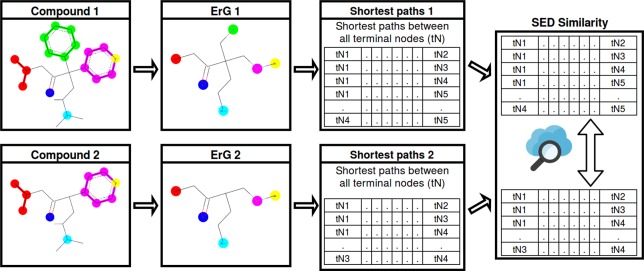
Harper et al. proposed another procedure to compare reduced graphs (Figure 4), in which the distance between two reduced graphs A and B is calculated by comparing the shortest paths between terminal nodes (nodes of degree one) in A and B. The distance between the two reduced graphs is defined as the maximum out of all of the minimum costs after all paths have been compared in A and B. When the paths are compared, some edition penalties are needed to balance the transformation from one node to another (or one edge to another). We have used the same transformation costs as those used for GED-based method (see below).
Figure 4.
SED-based method flowchart.
The SED-based similarity value presented in this study is computed with an in-house implementation that uses C++ and Python languages, following the steps described by Harper et al.36
GED-Based
Figure 5 shows a molecular comparison procedure using GED. GED is the most used method to solve error-tolerant graph matching. It defines a distance between graphs by determining the minimum number of modifications that are required to transform one graph into the other. To do so, these modifications, which are called edit operations, need to be defined. Basically, six different edit operations have been defined: insertion, deletion and substitution of both nodes and edges. In this way, for every pair of graphs A and B, there are several editPath(A,B) = (σ1,...,σk) that transforms one graph into the other, where each σi denotes an edit operation. Figure 6 shows a possible edit path that transforms graph A into graph B. It consists of the following 5 edit operations: delete edge, delete node, insert node, insert edge, and substitute node. The substitution operation is needed since the attributes of both nodes are different.
Figure 5.
GED-based method flowchart.
Figure 6.
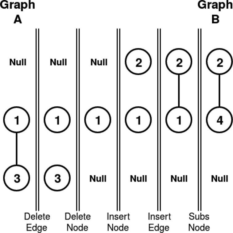
One of the edit paths that transforms graph A into graph B.
Edit costs have been introduced to quantitatively evaluate which edit path has the minimum total cost. The aim of these costs is to assign a transformation penalty to each edit operation depending on the extent to which it modifies the transformation sequence. The edit cost for a given edit path is the sum of all individual transformation costs. For instance, the edit cost for the edit path in Figure 6 is the cost of deleting an edge, plus the cost of deleting node 3, plus the cost of inserting node 2, plus the cost of inserting an edge, plus the cost of substitution from node 1 to node 4. The GED for any pair of graphs A and B is defined as the minimum cost under any possible edit path sequence of transforming one graph into the other.
The resulting distance is then adjusted according to the size of both graphs by dividing the obtained GED by their average number of nodes. The goal of this adjustment is to avoid favoring smaller graphs, since larger graphs tend to have larger overall transformation costs.
GED Computation
In the last three decades, a number of GED computation methods have been proposed. There are two types: those that return the exact value of the GED in exponential time with respect to the number of nodes,53 and those that return an approximation of the GED in polynomial time.54,55 These GED computation methods have been subject to studies and comparisons.56,57 An in-house implementation of the bipartite graph matching method proposed by Serratosa54 with C++ and Python languages was used to compute an approximation of the GED in polynomial time.
GED Costs
The edit costs should be selected depending on how similar the nodes and edges are. For instance, it is logical to think that, when ErGs are compared, the cost of substituting a hydrogen-bond donor feature with a joint hydrogen-bond donor–acceptor feature should be less heavily penalized than the cost of substituting a hydrogen-bond donor feature with an aromatic ring system. Similarly, inserting a single bond should have a lower cost than inserting a double bond and so on.
In this study we used the edit costs proposed by Harper et al.36 adapted to ErG. The node and edge descriptions are found in Table 1, and our specific costs can be observed in Table 2.
Table 1. Description of the Node and Edge Attributes That Make up an ErG.
| node attributes | |
|---|---|
| attribute | description |
| [0] | hydrogen-bond donor |
| [1] | hydrogen-bond acceptor |
| [2] | positive charge |
| [3] | negative charge |
| [4] | hydrophobic group |
| [5] | aromatic ring system |
| [6] | carbon link node |
| [7] | noncarbon link node |
| [0, 1] | hydrogen-bond donor + hydrogen-bond acceptor |
| [0, 2] | hydrogen-bond donor + positive charge |
| [0, 3] | hydrogen-bond donor + negative charge |
| [1, 2] | hydrogen-bond acceptor + positive charge |
| [1, 3] | hydrogen-bond acceptor + negative charge |
| [2, 3] | positive charge + negative charge |
| [0, 1, 2] | hydrogen-bond donor + hydrogen-bond acceptor + positive charge |
| edge attributes | |
| attribute | description |
| - | single bond |
| = | double bond |
| ≡ | triple bond |
Table 2. Substitution and Insertion/Deletion Costs Used in the GED and SED Calculation.
| matrix of substitution
costs | ||||||||||||||||||
|---|---|---|---|---|---|---|---|---|---|---|---|---|---|---|---|---|---|---|
| [0] | [1] | [2] | [3] | [4] | [5] | [6] | [7] | [0, 1] | [0, 2] | [0, 3] | [1, 2] | [1, 3] | [2, 3] | [0, 1, 2] | - | = | ≡ | |
| [0] | 0 | 2 | 2 | 2 | 2 | 2 | 2 | 3 | 1 | 1 | 1 | 2 | 2 | 2 | 1 | 2 | 3 | 3 |
| [1] | 2 | 0 | 2 | 2 | 2 | 2 | 2 | 3 | 1 | 2 | 2 | 1 | 1 | 2 | 1 | 2 | 3 | 3 |
| [2] | 2 | 2 | 0 | 2 | 2 | 2 | 2 | 3 | 2 | 1 | 2 | 1 | 2 | 1 | 1 | 2 | 3 | 3 |
| [3] | 2 | 2 | 2 | 0 | 2 | 2 | 2 | 3 | 2 | 2 | 1 | 2 | 1 | 1 | 2 | 2 | 3 | 3 |
| [4] | 2 | 2 | 2 | 2 | 0 | 2 | 2 | 3 | 2 | 2 | 2 | 2 | 2 | 2 | 2 | 2 | 3 | 3 |
| [5] | 2 | 2 | 2 | 2 | 2 | 0 | 2 | 3 | 2 | 2 | 2 | 2 | 2 | 2 | 2 | 2 | 3 | 3 |
| [6] | 2 | 2 | 2 | 2 | 2 | 2 | 0 | 3 | 2 | 2 | 2 | 2 | 2 | 2 | 2 | 2 | 3 | 3 |
| [7] | 3 | 3 | 3 | 3 | 3 | 3 | 3 | 0 | 3 | 3 | 3 | 3 | 3 | 3 | 3 | 3 | 3 | 3 |
| [0, 1] | 1 | 1 | 2 | 2 | 2 | 2 | 2 | 3 | 0 | 2 | 2 | 2 | 2 | 2 | 2 | 2 | 3 | 3 |
| [0, 2] | 1 | 2 | 1 | 2 | 2 | 2 | 2 | 3 | 2 | 0 | 2 | 2 | 2 | 2 | 2 | 2 | 3 | 3 |
| [0, 3] | 1 | 2 | 2 | 1 | 2 | 2 | 2 | 3 | 2 | 2 | 0 | 2 | 2 | 2 | 2 | 2 | 3 | 3 |
| [1, 2] | 2 | 1 | 1 | 2 | 2 | 2 | 2 | 3 | 2 | 2 | 2 | 0 | 2 | 2 | 2 | 2 | 3 | 3 |
| [1, 3] | 2 | 1 | 2 | 1 | 2 | 2 | 2 | 3 | 2 | 2 | 2 | 2 | 0 | 2 | 2 | 2 | 3 | 3 |
| [2, 3] | 2 | 2 | 1 | 1 | 2 | 2 | 2 | 3 | 2 | 2 | 2 | 2 | 2 | 0 | 2 | 2 | 3 | 3 |
| [0, 1, 2] | 1 | 1 | 1 | 2 | 2 | 2 | 2 | 3 | 2 | 2 | 2 | 2 | 2 | 2 | 0 | 2 | 3 | 3 |
| - | 2 | 2 | 2 | 2 | 2 | 2 | 2 | 3 | 2 | 2 | 2 | 2 | 2 | 2 | 2 | 0 | 3 | 3 |
| = | 3 | 3 | 3 | 3 | 3 | 3 | 3 | 3 | 3 | 3 | 3 | 3 | 3 | 3 | 3 | 3 | 0 | 3 |
| ≡ | 3 | 3 | 3 | 3 | 3 | 3 | 3 | 3 | 3 | 3 | 3 | 3 | 3 | 3 | 3 | 3 | 3 | 0 |
| insertion/deletion costs | ||||||||||||||||||
| insert | 1 | 1 | 1 | 1 | 1 | 1 | 0.5 | 0.5 | 1 | 1 | 1 | 1 | 1 | 1 | 1 | 0.1 | 1 | 1 |
| delete | 1 | 1 | 1 | 1 | 1 | 1 | 0.5 | 0.5 | 1 | 1 | 1 | 1 | 1 | 1 | 1 | 0.1 | 1 | 1 |
Method Evaluation
The LBVS benchmarking platform and the RDKit were used to evaluate the three methods mentioned before: fingerprint-based, SED-based, and GED-based. The screening phase consists of using all active and inactive compounds in the test set to be compared with the active compounds in the training set. Then, all test molecules are ranked according to their similarity to the active molecules in the training set, and only the information from the test molecule with the highest similarity value is kept. Subsequently, the performance of each method is calculated by using the information obtained in the previous step and some of the performance-evaluation methods.
As recommended by Riniker and Landrum in their fingerprint benchmarking study,48 it is good practice to provide the performance values for AUC and one of the “early recognition” methods, enrichment factor (EF) or Boltzmann-enhanced discrimination of ROC (BEDROC).58 In this study we selected the BEDROC (α = 20) as our “early recognition” method, since it has the advantage of running from 0 to 1.
Computational Expense
The evaluations reported in this study were performed using a quad-core, 2.0 GHz Intel Core i7 laptop with 8 GB RAM (operating system version Ubuntu 16.04). The most time-consuming step during the benchmarking process is calculating the similarity between graphs for each method; the remaining steps require negligible computational expense. An accurate time-consuming comparison would not be fair, since different methods were developed using different proportions of Python or C++ programming language. Nevertheless, for the data sets considered here, none of the similarity calculations took longer than 20 min per target (executing 10 iterations per target, each iteration performs almost 20 thousand individual molecular comparisons) using the predefined random-built splits available in the LBVS benchmarking platform.
Results
Experimental Setup
Six experiments were carried out using different activity classes from six publicly available data sets. The classification accuracy for the methods tested was computed using the screening and statistical tools available in the LBVS benchmarking platform and the RDKit. The AUC and BEDROC results obtained show the behavior of all the targets available in each data set in the platform using the Fingerprint-based, SED-based and GED-based methods.
Analysis of the Experiments
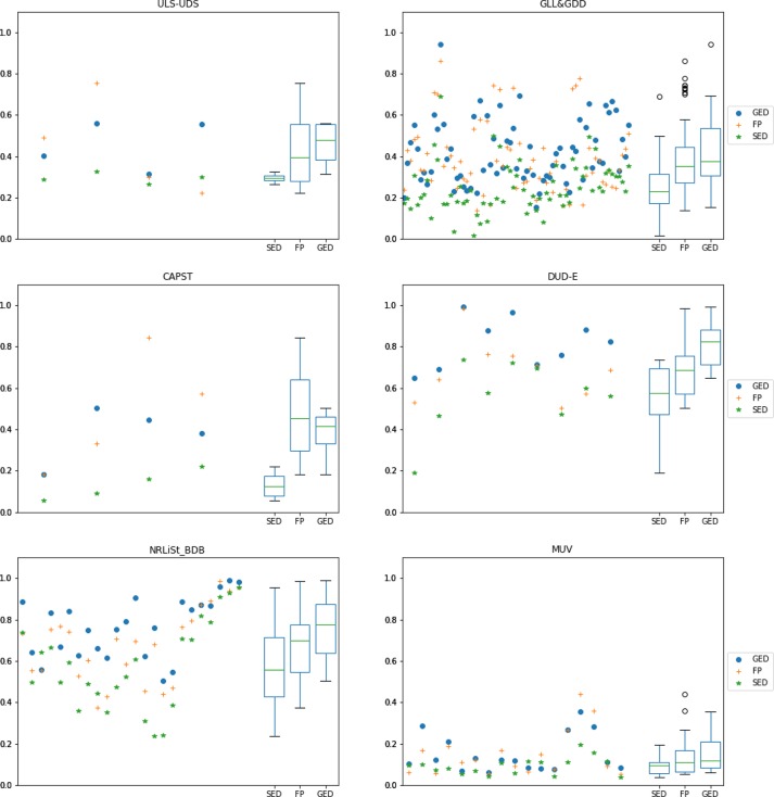
Table 3 summarizes the input data of the experiments, and Figure 7 shows the overall behavior for the three similarity methods for all of the targets available in the LBVS platform. These results show that the GED-based method has a slight advantage over the FP-based and the SED-based methods, which can be observed in the median, first quartile, and third quartile for both the AUC and BEDROC results in the box-and-whisker plots. An overall comparison might not be very informative, so a deeper analysis should be carried out for each data set separately.
Table 3. Input Data Used for the Experimentsa.
| data set | targets used |
|---|---|
| ULS-UDS | 5HT1F_Agonist, MTR1B_Agonist, OPRM_Agonist, PE2R3_Antagonist |
| GLL&GDD | 5HT1A_Agonist, 5HT1A_Antagonist, 5HT1D_Agonist, 5HT1D_Antagonist, 5HT1F_Agonist, 5HT2A_Antagonist, 5HT2B_Antagonist, 5HT2C_Agonist, 5HT2C_Antagonist, 5HT4R_Agonist, 5HT4R_Antagonist, AA1R_Agonist, AA1R_Antagonist, AA2AR_Antagonist, AA2BR_Antagonist, ACM1_Agonist, ACM2_Antagonist, ACM3_Antagonist, ADA1A_Antagonist, ADA1B_Antagonist, ADA1D_Antagonist, ADA2A_Agonist, ADA2A_Antagonist, ADA2B_Agonist, ADA2B_Antagonist, ADA2C_Agonist, ADA2C_Antagonist, ADRB1_Agonist, ADRB1_Antagonist, ADRB2_Agonist, ADRB2_Antagonist, ADRB3_Agonist, ADRB3_Antagonist, AG2R_Antagonist, BKRB1_Antagonist, BKRB2_Antagonist, CCKAR_Antagonist, CLTR1_Antagonist, DRD1_Antagonist, DRD2_Agonist, DRD2_Antagonist, DRD3_Antagonist, DRD4_Antagonist, EDNRA_Antagonist, EDNRB_Antagonist, GASR_Antagonist, HRH2_Antagonist, HRH3_Antagonist, LSHR_Antagonist, LT4R1_Antagonist, LT4R2_Antagonist, MTR1A_Agonist, MTR1B_Agonist, MTR1L_Agonist, NK1R_Antagonist, NK2R_Antagonist, NK3R_Antagonist, OPRD_Agonist, OPRK_Agonist, OPRM_Agonist, OXYR_Antagonist, PE2R1_Antagonist, PE2R2_Antagonist, PE2R3_Antagonist, PE2R4_Antagonist, TA2R_Antagonist, V1AR_Antagonist, V1BR_Antagonist, V2R_Antagonist |
| CAPST | CDK2, CHK1, PTP1B, UROKINASE |
| DUD-E | COX2, DHFR, EGFR, FGFR1, FXA, P38, PDGFRB, SRC, AA2AR |
| NRLiSt_BDB | AR_Agonist, AR_Antagonist, ER_Alpha_Agonist, ER_Alpha_Antagonist, ER_Beta_Agonist, FXR_Alpha_Agonist, GR_Agonist, GR_Antagonist, LXR_Alpha_Agonist, LXR_Beta_Agonist, MR_Antagonist, PPAR_Alpha_Agonist, PPAR_Beta_Agonist, PPAR_Gamma_Agonist, PR_Agonist, PR_Antagonist, PXR_Agonist, RAR_Alpha_Agonist, RAR_Beta_Agonist, RAR_Gamma_Agonist, RXR_Alpha_Agonist, RXR_Alpha_Antagonist, RXR_Gamma_Agonist, VDR_Agonist |
| MUV | 466, 548, 600, 644, 652, 689, 692, 712, 713, 733, 737, 810, 832, 846, 852, 858, 859 |
The column entitled “dataset” contains the name of each dataset, and the column entitled “targets used” contains the name of the targets used during the experiments for each dataset. Note that in result plots shown below, per-target points are arranged in the same order as they are in this table.
Figure 7.
AUC and BEDROC (α = 20) over all available targets in the LBVS benchmarking platform. The scattered values on the left of both subplots represent the median value from 10 predefined random-built splits, using different colors and shapes per similarity method. Vertical segmented lines mark the edge between different data sets (from left to right: ULS-UDS, GLL&GDD, CAPST, DUD-E, NRLiSt_BDB, and MUV). The box-and-whisker plots on the right of both subplots show the distribution of the resulting values for each similarity method. The boxes show the first and third quartile, the line is the median value (second quartile), and the whiskers extend from the boxes to show the range of the data (outliers are included if there are any).
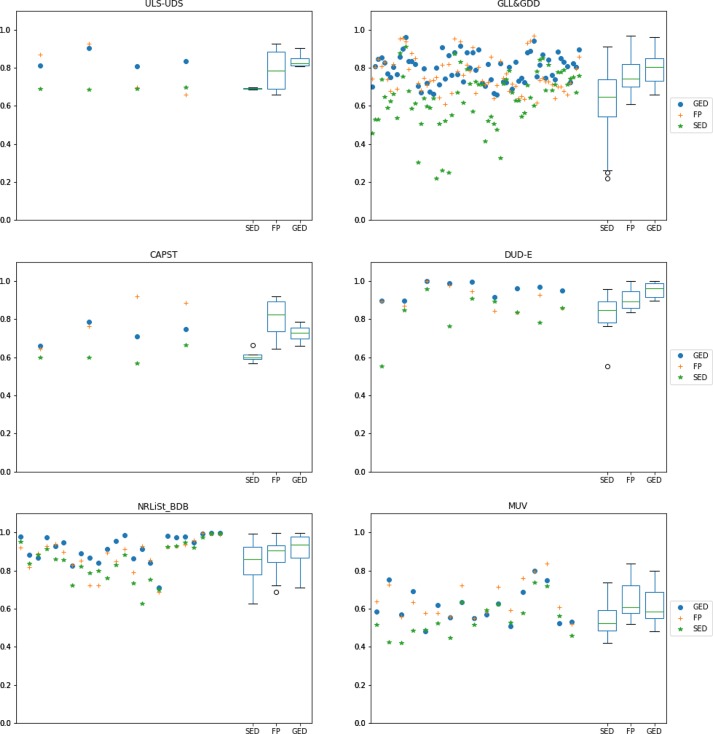
Figures 8 and 9 show the same information as Figure 7, but this time the specific behavior for each data set can be seen separately (one data set per subfigure). Figure 8 represents the AUC values, and Figure 9 represents the BEDROC values. Again, box-and-whisker plots are located on the right of each subplot to illustrate the distribution of the values. The following analysis will focus on these distribution results.
Figure 8.
AUC results for all available targets in the LBVS benchmarking platform separated by data set. Each scattered value on the left of each subplot represents the median value of 10 predefined random-built splits. A different color and shape is used for each similarity method. Box-and-whisker plots on the right of each subplot show the distribution of the resulting values for each similarity method.
Figure 9.
BEDROC (α = 20) results for all available targets in the LBVS benchmarking platform separated by data set. Each scattered value on the left of each subplot represents the median value of 10 predefined random-built splits. A different color and shape is used for each similarity method. Box-and-whisker plots on the right of each subplot show the distribution of the resulting values for each similarity method.
For the ULS-UDS data set, the median value of results for the GED-based method is better than for the FP-based and SED-based methods. This is noticeable in the AUC and BEDROC results, specially in the last two targets (OPRM_Agonist and PE2R3_Antagonist). Probably the most noticeable advantage of the GED-based method in this case is its stability (stability is represented as the box and whiskers length; shorter lengths indicate that several results are closer to each other so the method seems more reliable).
For the GLL&GDD data set, the performance of the GED-based method is significantly better than of the FP-based and SED-based methods. The median, first quartile and third quartile are better in both the AUC and BEDROC results. The biggest difference in performance can be noticed in the “PE2R” group targets, located close to the right in the plot (PE2R1_Antagonist, PE2R2_Antagonist, PE2R3_Antagonist and PE2R4_Antagonist).
For the CAPST data set, the performance is slightly better for the FP-based method than for the GED-based and SED-based methods. This can be seen in the AUC and BEDROC results. The better FP-based performance is more noticeable in the last two targets (PTP1B and UROKINASE). Nevertheless, the stability of results is not very reliable, specially in BEDROC, where performance goes from very low to very high values.
The advantage of the GED-based method is possibly greatest for the DUD-E data set. Even the second quartile of the GED-based method is higher than the third quartile of the FP-based and SED-based methods. This is true for the AUC and BEDROC values. Besides, the GED-based method is quite stable, particularly for the AUC values. The GED-based superiority is more noticeable in such targets as P38, SRC, FXA and FGFR1 located between the center and the right of the plot.
For the NRLiSt_BDB data set, again the GED-based method gets significantly better results than the FP-based and SED-based methods. This can be seen in the AUC and BEDROC results, and it is evident in the first, second (median) and third quartiles. The stability is similar for all methods, with the FP-based method being slightly better in the AUC values and the SED-based method being slightly better in the BEDROC values. The biggest difference between the performance of the GED-based method and the performance of the other methods can be observed in such targets as LXR_Alpha_Agonist, LXR_Beta_Agonist, PPAR_Alpha_Agonist, and PPAR_Gamma_Agonist, near the center of the plot.
The overall results for the MUV data set are the lowest of all of the experiments. This is true for all three similarity methods. Nevertheless, the GED-based method performs slightly better than the FP-based and the SED-based methods in the “early recognition” BEDROC results. The difference is more significant for such targets as 466, 548, and 600 on the left of the plot. The FP-based method performs slightly better than others in the AUC results, particularly in such targets as 652, 852 and 737.
Statistical Tests
As well as the above analysis, statistical tests were carried out to determine whether the differences in performance are statistically significant. In other words, these tests assess whether some methods are consistently better than others.
The first step used the overall Friedman test.59Table 4 shows the overall Friedman test results for each data set. The last row shows the results of applying the same test to all of the targets combined. The p-value of the overall Friedman test was extremely low in most cases (a confidence level of α = 0.05 is used), which indicates that there are statistically significant differences between different methods. Hence, a more in-depth analysis might be helpful.
Table 4. P-Values of a Friedman Test for AUC and BEDROC Results, Comparing All Three Similarity Methods (GED-Based, FP-Based, and SED-Based) at the Same Timea.
| Friedman test (AUC) | Friedman test (BEDROC) | |
|---|---|---|
| ULS-UDS | 0.173774 | 0.173774 |
| GLL&GDD | 2.97804 × 10⁻¹⁴* | 5.30798 × 10⁻¹⁵* |
| DUD-E | 0.000911882* | 0.000300185* |
| NRLiSt_BDB | 7.48518 × 10–05* | 5.77775 × 10–08* |
| MUV | 0.00102573* | 0.00714619* |
| CAPST | 0.0497871* | 0.0497871* |
| all data sets | 7.46387 × 10⁻²⁴* | 1.89219 × 10⁻²⁸* |
The test is done per dataset, and all datasets are combined in the last row. Here, a confidence level of α = 0.05 is used, so p-values lower than α indicate statistically significant differences, which are marked with an asterisk (*) in the table.
The second step in the statistical tests consists of a pairwise Wilcoxon signed-rank test60 to determine which pairs of methods exhibit a statistically significant difference. Table 5 shows the results of this test applied to all of the data sets combined and using the AUC and BEDROC results.
Table 5. P-Values of a Pairwise Wilcoxon Signed-Rank Test for AUC and BEDROC Results, Comparing All Three Similarity Methods (GED-Based, FP-Based, and SED-Based)a.
| Wilcoxon test (AUC) |
Wilcoxon test (BEDROC) |
|||||
|---|---|---|---|---|---|---|
| SED | FP | GED | SED | FP | GED | |
| SED | 1.20841 × 10⁻¹³* | 7.4432 × 10⁻²¹* | 2.08456 × 10⁻¹⁶* | 1.18024 × 10⁻²¹* | ||
| FP | 1.20841 × 10⁻¹³* | 0.000748788* | 2.08456 × 10⁻¹⁶* | 0.000585085* | ||
| GED | 7.4432 × 10⁻²¹* | 0.000748788* | 1.18024 × 10⁻²¹* | 0.000585085* | ||
The test is applied to all targets in the datasets combined. Here, a confidence level of α = 0.05 is used, so p-values lower than α indicate statistically significant differences, which are marked with an asterisk (*) in the table.
The same pairwise Wilcoxon signed-rank test was performed again but this time applied to each data set separately. The results of the tests are presented in Tables 6 (AUC values) and 7 (BEDROC values).
Table 6. P-Values of a Pairwise Wilcoxon Signed-Rank Test for AUC Results, Comparing All Three Similarity Methods (GED-Based, FP-Based, and SED-Based)a.
| ULS-UDS |
GLL&GDD |
|||||
|---|---|---|---|---|---|---|
| SED | FP | GED | SED | FP | GED | |
| SED | 0.273322 | 0.0678892 | 4.26037 × 10–08* | 3.34327 × 10⁻¹²* | ||
| FP | 0.273322 | 0.465209 | 4.26037 × 10–08* | 0.0018207* | ||
| GED | 0.0678892 | 0.465209 | 3.34327 × 10⁻¹²* | 0.0018207* | ||
| CAPST |
MUV |
|||||
|---|---|---|---|---|---|---|
| SED | FP | GED | SED | FP | GED | |
| SED | 0.0678892 | 0.0678892 | 0.000351533* | 0.00748178* | ||
| FP | 0.0678892 | 0.465209 | 0.000351533* | 0.0615039 | ||
| GED | 0.0678892 | 0.465209 | 0.00748178* | 0.0615039 | ||
| DUD-E |
NRLiSt_BDB |
|||||
|---|---|---|---|---|---|---|
| SED | FP | GED | SED | FP | GED | |
| SED | 0.109745 | 0.00768579* | 0.0520334 | 3.02696 × 10–05* | ||
| FP | 0.109745 | 0.00768579* | 0.0520334 | 0.00167307* | ||
| GED | 0.00768579* | 0.00768579* | 3.02696 × 10–05* | 0.00167307* | ||
The test is done using all targets separated by datasets. Here, a confidence level of α = 0.05 is used, so p-values lower than α indicate statistically significant differences, which are marked with an asterisk (*) in the table.
Pairwise comparison tables show very low p-values in most cases (the lower the p-value the better), and the difference between one method and the other was statistically significant. This is true for AUC and BEDROC results and for all data sets except ULS-UDS and CAPST. Therefore, for these two data sets, the slight differences in performance are not regarded as statistically significant. Note that statistically significant differences may not always mean practically meaningful differences (Table 7).61
Table 7. P-Values of a Pairwise Wilcoxon Signed-Rank Test for BEDROC Results, Comparing All Three Similarity Methods (GED-Based, FP-Based, and SED-Based)a.
| ULS-UDS | GLL&GDD | |||||
|---|---|---|---|---|---|---|
| SED | FP | GED | SED | FP | GED | |
| SED | 0.273322 | 0.0678892 | 1.41571 × 10–09* | 7.73521 × 10⁻¹³* | ||
| FP | 0.273322 | 1 | 1.41571 × 10–09* | 0.125128 | ||
| GED | 0.0678892 | 1 | 7.73521 × 10⁻¹³* | 0.125128 | ||
| CAPST | MUV | |||||
| SED | FP | GED | SED | FP | GED | |
| SED | 0.0678892 | 0.0678892 | 0.00988213* | 0.00359936* | ||
| FP | 0.0678892 | 0.465209 | 0.00988213* | 0.758312 | ||
| GED | 0.0678892 | 0.465209 | 0.00359936* | 0.758312 | ||
| DUD-E | NRLiSt_BDB | |||||
| SED | FP | GED | SED | FP | GED | |
| SED | 0.015156* | 0.00768579* | 0.000318217* | 3.43006 × 10–05* | ||
| FP | 0.015156* | 0.00768579* | 0.000318217* | 0.000284994* | ||
| GED | 0.00768579* | 0.00768579* | 3.43006 × 10–05* | 0.000284994* | ||
The test is done using all targets separated by datasets. Here, a confidence level of α = 0.05 is used, so p-values lower than α indicate statistically significant differences, which are marked with an asterisk (*) in the table.
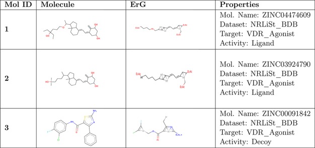
Finally, Table 8 shows the drawing and the ErG representation of three sample molecules. As an example, we selected the first two active molecules (ligands) and the first inactive molecule (decoy) from the target VDR_Agonist in the NRLiSt_BDB data set. Table 9 shows the distances between these molecules using the FP-based, SED-based, and GED-based similarity methods. The range of FP-based and SED-based distances is [0,1] whereas the range of the GED-based is [0,Inf]. Hence, the values obtained with different methods cannot be compared. Nevertheless, it is noticeable that, for each method, the distance value computed between two ligand compounds is lower than the distance computed between a ligand compound and a decoy compound. This is the basis of correctly classifying the ligand and decoy molecules to be used in the process of virtual screening.
Table 8. Three Sample Molecules from the Target VDR_Agonist in the NRLiSt_BDB Dataset.
Table 9. Distances between Molecules Shown in Table 8 Computed Using the FP-Based, SED-Based, and GED-Based Similarity Methods.
| Mol ID 2 ligand | Mol ID 3 decoy | |
|---|---|---|
| Mol ID 1 ligand | SED: 0.06 | SED: 0.28 |
| FPD: 0.40 | FPD: 0.92 | |
| GED: 0.49 | GED: 3.05 |
Conclusions and Future Research
This paper presents a molecular similarity measure that uses graph edit distance to effectively compare the representation of molecules by extended reduced graphs. This method works as an alternative to the fingerprint-based similarity method used in the original paper on ErGs by Stiefl et al. and also as an alternative to the string edit distance-based method used in the paper by Harper et al.
The experiments performed used several samples collected from publicly available data sets like DUD-E and MUV. To overcome the common problems of reproducibility when different methods are compared, we used a benchmarking platform proposed by Skoda and Hoksza which, among other features, includes several screening and statistical tools and provides fully reproducible outcomes.
The results of the experiments show that the GED-based method performed better in 4 out of 6 methods according to AUC and in 5 out of 6 methods according to the “early recognition” BEDROC. Nevertheless, these differences are statistically significant in four of the data sets, since for ULS-UDS and CAPST, the differences are not significant according to the pairwise Wilcoxon signed-rank test.
To compute the GED, we used the edit costs proposed by Harper et al. which were assigned by experts to manage relationships between different node and edge types. Further research will focus on automatically learning the edit costs on nodes and edges in several scenarios using a variety of toxicological end points. This learning process will be similar to that carried out by Birchall et al.62 in which they optimized the edit values proposed by Harper et al. for their method.
For purposes of simplicity, the GED implementation used in this study does not envisage the use of stereochemical information for molecules. This issue could be addressed in future studies. It should be possible to include this information since the 3D location of each atom is available for all of the data sets in the LBVS benchmarking platform, so a reference for the position of the neighbors with respect to each atom should be able to be established.
Acknowledgments
This project has received funding from the European Union’s Horizon 2020 research and innovation programme under the Marie Skłodowska-Curie grant agreement No. 713679 and from the Universitat Rovira i Virgili (URV). This study has also been partially supported by the European project NanoDesk (SOE1/P1/E0215); the Spanish projects TIN2016-77836-C2-1-R and ColRobTransp MINECO DPI2016-78957-R AEI/FEDER EU; and also by the European project AEROARMS, H2020-ICT-2014-1-644271.
The authors declare no competing financial interest.
References
- Kubinyi H.; Mannhold R.; Timmerman H.. Virtual screening for bioactive molecules; John Wiley & Sons: New York, 2008; Vol. 10. [Google Scholar]
- Schneider G.; Clément-Chomienne O.; Hilfiger L.; Schneider P.; Kirsch S.; Böhm H.-J.; Neidhart W. Virtual screening for bioactive molecules by evolutionary de novo design. Angew. Chem., Int. Ed. 2000, 39, 4130–4133. . [DOI] [PubMed] [Google Scholar]
- Bajorath J. Selected concepts and investigations in compound classification, molecular descriptor analysis, and virtual screening. J. Chem. Inf. Comput. Sci. 2001, 41, 233–245. 10.1021/ci0001482. [DOI] [PubMed] [Google Scholar]
- Heikamp K.; Bajorath J. The future of virtual compound screening. Chem. Biol. Drug Des. 2013, 81, 33–40. 10.1111/cbdd.12054. [DOI] [PubMed] [Google Scholar]
- Cereto-Massagué A.; Ojeda M. J.; Valls C.; Mulero M.; Garcia-Vallvé S.; Pujadas G. Molecular fingerprint similarity search in virtual screening. Methods 2015, 71, 58–63. 10.1016/j.ymeth.2014.08.005. [DOI] [PubMed] [Google Scholar]
- Sun H. Pharmacophore-based virtual screening. Curr. Med. Chem. 2008, 15, 1018–1024. 10.2174/092986708784049630. [DOI] [PubMed] [Google Scholar]
- Kirchmair J.; Distinto S.; Markt P.; Schuster D.; Spitzer G. M.; Liedl K. R.; Wolber G. How to optimize shape-based virtual screening: choosing the right query and including chemical information. J. Chem. Inf. Model. 2009, 49, 678–692. 10.1021/ci8004226. [DOI] [PubMed] [Google Scholar]
- Melville J. L.; Burke E. K.; Hirst J. D. Machine learning in virtual screening. Comb. Chem. High Throughput Screening 2009, 12, 332–343. 10.2174/138620709788167980. [DOI] [PubMed] [Google Scholar]
- Johnson M. A.; Maggiora G. M.. Concepts and applications of molecular similarity; Wiley: New York, 1990. [Google Scholar]
- Bender A.; Glen R. C. Molecular similarity: a key technique in Mol. Inf. Org. Biomol. Chem. 2004, 2, 3204–3218. 10.1039/b409813g. [DOI] [PubMed] [Google Scholar]
- Nikolova N.; Jaworska J. Approaches to measure chemical similarity–a review. QSAR Comb. Sci. 2003, 22, 1006–1026. 10.1002/qsar.200330831. [DOI] [Google Scholar]
- Willett P.Chemoinformatics; Springer: Berlin, 2004; pp 51–63. [Google Scholar]
- Lajiness M.Molecular similarity-based methods for selecting compounds for screening. Computational chemical graph theory; 1990; pp 299–316. [Google Scholar]
- Willett J.Similarity and clustering in chemical information systems; John Wiley & Sons, Inc.: New York, 1987. [Google Scholar]
- Sheridan R. P.; Kearsley S. K. Why do we need so many chemical similarity search methods?. Drug Discovery Today 2002, 7, 903–911. 10.1016/S1359-6446(02)02411-X. [DOI] [PubMed] [Google Scholar]
- Willett P.; Barnard J. M.; Downs G. M. Chemical similarity searching. J. Chem. Inf. Comput. Sci. 1998, 38, 983–996. 10.1021/ci9800211. [DOI] [Google Scholar]
- Xue L.; Bajorath J. Molecular descriptors in chemoinformatics, computational combinatorial chemistry, and virtual screening. Comb. Chem. High Throughput Screening 2000, 3, 363–372. 10.2174/1386207003331454. [DOI] [PubMed] [Google Scholar]
- Menard P. R.; Mason J. S.; Morize I.; Bauerschmidt S. Chemistry space metrics in diversity analysis, library design, and compound selection. J. Chem. Inf. Comput. Sci. 1998, 38, 1204–1213. 10.1021/ci9801062. [DOI] [Google Scholar]
- Pearlman R. S.; Smith K. M. Metric validation and the receptor-relevant subspace concept. J. Chem. Inf. Comput. Sci. 1999, 39, 28–35. 10.1021/ci980137x. [DOI] [Google Scholar]
- Schnur D. Design and diversity analysis of large combinatorial libraries using cell-based methods. J. Chem. Inf. Comput. Sci. 1999, 39, 36–45. 10.1021/ci980138p. [DOI] [Google Scholar]
- Livingstone D. J. The characterization of chemical structures using molecular properties. A survey. J. Chem. Inf. Comput. Sci. 2000, 40, 195–209. 10.1021/ci990162i. [DOI] [PubMed] [Google Scholar]
- Barnard J. M. Substructure searching methods: Old and new. J. Chem. Inf. Model. 1993, 33, 532–538. 10.1021/ci00014a001. [DOI] [Google Scholar]
- James C.; Weininger D.. Daylight, 4.41 Theory Manual; Daylight Chemical Information Systems Inc.: Irvine, CA, 1995. [Google Scholar]
- MACCS K.MDL Information Systems. Inc.: San Leandro, CA, 1984. [Google Scholar]
- McGregor M. J.; Pallai P. V. Clustering of large databases of compounds: using the MDL ‘‘keys” as structural descriptors. J. Chem. Inf. Comput. Sci. 1997, 37, 443–448. 10.1021/ci960151e. [DOI] [Google Scholar]
- Güner O. F.Pharmacophore perception, development, and use in drug design; Internat’l University Line, 2000; Vol. 2. [Google Scholar]
- Beno B. R.; Mason J. S. The design of combinatorial libraries using properties and 3D pharmacophore fingerprints. Drug Discovery Today 2001, 6, 251–258. 10.1016/S1359-6446(00)01665-2. [DOI] [PubMed] [Google Scholar]
- Rarey M.; Dixon J. S. Feature trees: a new molecular similarity measure based on tree matching. J. Comput.-Aided Mol. Des. 1998, 12, 471–490. 10.1023/A:1008068904628. [DOI] [PubMed] [Google Scholar]
- Takahashi Y.; Sukekawa M.; Sasaki S. Automatic identification of molecular similarity using reduced-graph representation of chemical structure. J. Chem. Inf. Model. 1992, 32, 639–643. 10.1021/ci00010a009. [DOI] [Google Scholar]
- Barker E. J.; Buttar D.; Cosgrove D. A.; Gardiner E. J.; Kitts P.; Willett P.; Gillet V. J. Scaffold hopping using clique detection applied to reduced graphs. J. Chem. Inf. Model. 2006, 46, 503–511. 10.1021/ci050347r. [DOI] [PubMed] [Google Scholar]
- Fisanick W.; Lipkus A. H.; Rusinko A. Similarity Searching on CAS Registry Substances. 2. 2D Structural Similarity. J. Chem. Inf. Model. 1994, 34, 130–140. 10.1021/ci00017a016. [DOI] [Google Scholar]
- Gillet V. J.; Downs G. M.; Holliday J. D.; Lynch M. F.; Dethlefsen W. Computer storage and retrieval of generic chemical structures in patents. 13. Reduced graph generation. J. Chem. Inf. Model. 1991, 31, 260–270. 10.1021/ci00002a011. [DOI] [Google Scholar]
- Gillet V. J.; Willett P.; Bradshaw J. Similarity searching using reduced graphs. J. Chem. Inf. Comput. Sci. 2003, 43, 338–345. 10.1021/ci025592e. [DOI] [PubMed] [Google Scholar]
- Stiefl N.; Watson I. A.; Baumann K.; Zaliani A. ErG: 2D pharmacophore descriptions for scaffold hopping. J. Chem. Inf. Model. 2006, 46, 208–220. 10.1021/ci050457y. [DOI] [PubMed] [Google Scholar]
- Barker E. J.; Gardiner E. J.; Gillet V. J.; Kitts P.; Morris J. Further development of reduced graphs for identifying bioactive compounds. J. Chem. Inf. Comput. Sci. 2003, 43, 346–356. 10.1021/ci0255937. [DOI] [PubMed] [Google Scholar]
- Harper G.; Bravi G. S.; Pickett S. D.; Hussain J.; Green D. V. S. The reduced graph descriptor in virtual screening and data-driven clustering of high-throughput screening data. J. Chem. Inf. Comput. Sci. 2004, 44, 2145–2156. 10.1021/ci049860f. [DOI] [PubMed] [Google Scholar]
- Munkres J. Algorithms for the Assignment and Transportation Problems. J. Soc. Ind. Appl. Math. 1957, 5, 32–38. 10.1137/0105003. [DOI] [Google Scholar]
- Sanfeliu A.; Fu K.-S. A distance measure between attributed relational graphs for Pattern Recognit. IEEE transactions on systems, man, and cybernetics 1983, SMC-13, 353–362. 10.1109/TSMC.1983.6313167. [DOI] [Google Scholar]
- Gao X.; Xiao B.; Tao D.; Li X. A survey of graph edit distance. Pattern Analysis and applications 2010, 13, 113–129. 10.1007/s10044-008-0141-y. [DOI] [Google Scholar]
- Solé A.; Serratosa F.; Sanfeliu A. On the Graph Edit Distance Cost: Properties and Applications. Intern. Int. J. Patt. Recognit. Artif. Intell. 2012, 26, 1260004. 10.1142/S021800141260004X. [DOI] [Google Scholar]
- Xia J.; Tilahun E. L.; Reid T.-E.; Zhang L.; Wang X. S. Benchmarking methods and data sets for ligand enrichment assessment in virtual screening. Methods 2015, 71, 146–157. 10.1016/j.ymeth.2014.11.015. [DOI] [PMC free article] [PubMed] [Google Scholar]
- Gatica E. A.; Cavasotto C. N. Ligand and decoy sets for docking to G protein-coupled receptors. J. Chem. Inf. Model. 2012, 52, 1–6. 10.1021/ci200412p. [DOI] [PubMed] [Google Scholar]
- Mysinger M. M.; Carchia M.; Irwin J. J.; Shoichet B. K. Directory of useful decoys, enhanced (DUD-E): better ligands and decoys for better benchmarking. J. Med. Chem. 2012, 55, 6582–6594. 10.1021/jm300687e. [DOI] [PMC free article] [PubMed] [Google Scholar]
- Lagarde N.; Ben Nasr N.; Jeremie A.; Guillemain H.; Laville V.; Labib T.; Zagury J.-F.; Montes M. NRLiSt BDB, the manually curated nuclear receptors ligands and structures benchmarking database. J. Med. Chem. 2014, 57, 3117–3125. 10.1021/jm500132p. [DOI] [PubMed] [Google Scholar]
- Rohrer S. G.; Baumann K. Maximum unbiased validation (MUV) data sets for virtual screening based on PubChem bioactivity data. J. Chem. Inf. Model. 2009, 49, 169–184. 10.1021/ci8002649. [DOI] [PubMed] [Google Scholar]
- Sanders M. P.; Barbosa A. J.; Zarzycka B.; Nicolaes G. A.; Klomp J. P.; de Vlieg J.; Del Rio A. Comparative analysis of pharmacophore screening tools. J. Chem. Inf. Model. 2012, 52, 1607–1620. 10.1021/ci2005274. [DOI] [PubMed] [Google Scholar]
- Skoda P.; Hoksza D.. Benchmarking platform for ligand-based virtual screening. Proceedings - 2016 IEEE International Conference on Bioinformatics and Biomedicine; BIBM 2016, 2017; pp 1220–1227. [Google Scholar]
- Riniker S.; Landrum G. A. Open-source platform to benchmark fingerprints for ligand-based virtual screening. J. Cheminf. 2013, 5, 26. 10.1186/1758-2946-5-26. [DOI] [PMC free article] [PubMed] [Google Scholar]
- Brown C. D.; Davis H. T. Receiver operating characteristics curves and related decision measures: A tutorial. Chemom. Intell. Lab. Syst. 2006, 80, 24–38. 10.1016/j.chemolab.2005.05.004. [DOI] [Google Scholar]
- Kearsley S. K.; Sallamack S.; Fluder E. M.; Andose J. D.; Mosley R. T.; Sheridan R. P. Chemical similarity using physiochemical property descriptors. J. Chem. Inf. Comput. Sci. 1996, 36, 118–127. 10.1021/ci950274j. [DOI] [Google Scholar]
- Carhart R. E.; Smith D. H.; Venkataraghavan R. Atom pairs as molecular features in structure-activity studies: definition and applications. J. Chem. Inf. Model. 1985, 25, 64–73. 10.1021/ci00046a002. [DOI] [Google Scholar]
- RDKit: Cheminformatics and Machine Learning Software; http://www.rdkit.org, 2013. [Google Scholar]
- Blumenthal D. B.; Gamper J. On the exact computation of the graph edit distance. Pattern Recognit. Lett. 2018, 0, 1–12. 10.1016/j.patrec.2018.05.002. [DOI] [Google Scholar]
- Serratosa F. Fast computation of bipartite graph matching. Pattern Recognit. Lett. 2014, 45, 244–250. 10.1016/j.patrec.2014.04.015. [DOI] [Google Scholar]
- Santacruz P.; Serratosa F. Error-tolerant graph matching in linear computational cost using an initial small partial matching. Pattern Recognit. Lett. 2018, 0, 1–10. 10.1016/j.patrec.2018.04.003. [DOI] [Google Scholar]
- Conte D.; Foggia P.; Sansone C.; Vento M. Thirty years of graph matching in Pattern Recognit. Int. Journal of Pattern Recognit. and Artificial Intell. 2004, 18, 265–298. 10.1142/S0218001404003228. [DOI] [Google Scholar]
- Vento M. A long trip in the charming world of graphs for Pattern Recognit. Pattern Recognit 2015, 48, 291–301. 10.1016/j.patcog.2014.01.002. [DOI] [Google Scholar]
- Truchon J.-F.; Bayly C. I. Evaluating virtual screening methods: good and bad metrics for the ‘‘early recognition’’ problem. J. Chem. Inf. Model. 2007, 47, 488–508. 10.1021/ci600426e. [DOI] [PubMed] [Google Scholar]
- Friedman M. The use of ranks to avoid the assumption of normality implicit in the analysis of variance. J. Am. Stat. Assoc. 1937, 32, 675–701. 10.1080/01621459.1937.10503522. [DOI] [Google Scholar]
- Wilcoxon F. Individual comparisons by ranking methods. Biom. Bull. 1945, 1, 80–83. 10.2307/3001968. [DOI] [Google Scholar]
- Kenny P. W.; Montanari C. A. Inflation of correlation in the pursuit of drug-likeness. J. Comput.-Aided Mol. Des. 2013, 27, 1–13. 10.1007/s10822-012-9631-5. [DOI] [PubMed] [Google Scholar]
- Birchall K.; Gillet V. J.; Harper G.; Pickett S. D. Training similarity measures for specific activities: application to reduced graphs. J. Chem. Inf. Model. 2006, 46, 577–586. 10.1021/ci050465e. [DOI] [PubMed] [Google Scholar]


