Determination of an inflection point for a dosimetric analysis of unflattened beam using the first principle of derivatives by python code programming

Abstract

Background

Practice of Unflattened or Flattening filter free (FFF) beam has become the high dose standard in radiotherapy (RT), such as stereotactic radio-surgery (SRS) and stereotactic radiotherapy (SRT). The removal of a flattening filter (FF) from the path of a photon beam alters the characteristics of FFF beam. Since the conventional route for dosimetric analysis of FF beam cannot be applied to FFF beam, the procedure of analyzing beam characteristics for FFF beam based on inflection points (IPs) is used. IP is a point where the concavity change observed corresponds to its change in sign (±) of the second derivative.

Aim

The objective of the study is to determine IPs for dosimetric analysis of the FFF beam profile.

Methods and materials

In this study, IPs are determined through the python code programming based on the mathematical first principle of the derivative. They are compared with IPs estimated by the conventional graphical manual method using Microsoft Excel (MS). IPs and their dependent dosimetric parameters determined by both mathematical and graphical manual methods are compared.

Result

Percentage differences between the IPs determined by both methods, for 6MVFFF inline and crossline beam profile are found to be 2.7% and 0.8% respectively. Similarly, the average penumbra differences for 6MVFFF inline and crossline beam profile are found to be 0.15 mm and 0.9 mm, respectively. However, differences in the field width between both methods are found insignificant.

Conclusion

Graphical manual method is very time-consuming, tedious and user dependent. However, the mathematical method through python code programming is more precise, faster and independent of individual users.

1. Background

The practice of Unflattened or Flattening filter free (FFF) beam has become the golden standard in the treatment high dose radiotherapy (RT) like stereotactic radio-surgery (SRS) and stereotactic radiotherapy (SRT) as it can deliver high dose per fraction. Removal of the flattening filter from the path of a photon beam produces non-uniform intensity pattern along the cross section of the clinically useful beam profile. This significantly increases the dose rate as well as reduces the scatter, off-axis doses and head leakage for the photon beam. In addition to that, the reduction in neutron production is also observed.1, 2, 3 The idea behind the removal of a flattening filter (FF) is to reduce the treatment time by increasing the dose rate which could predominantly be achieved by removing FF.⁴ Absence of the FF also causes the softening of the beam spectra, which leads to a change in beam quality of FFF beam as well.⁵ In addition to that, FF beam needed high positional precision for maintaining the symmetry and flatness. Well, conventional radiation therapy techniques are replaced with modern automated static segmented and dynamic delivery by Multileaf Collimator (MLC). MLC delivers the treatment by generating an inhomogeneous fluence map. Thus, uniform fluence of a flat beam is not strictly necessary for the high-end technique like SRS and SRT. Even, at the field dimension of such techniques, the beam is acceptably flat without FF. Hence, for such high dose advance radiation therapy techniques, FF is not at all required.6, 7, 8

However, the difficulty associated with FFF beam is its forward peak geometry and maintaining dosimetric parameter for clinical use. The beam softening effect along the off-axis of a beam profile causes a sigmoid or S-shaped curve on either side of the beam profile. Preserving the shape of the curve is necessary, because this governs the symmetry and degree of unflatness for the geometry of forward peak intensity of the beam. This kind of curves is very common in many disciplines like Graph Theory, Biological Science, Analytical Chemistry, Dose response, etc. An essential key concept of the sigmoid curve is the inflection points (IPs).⁹ IP is a point where concavity changes and second derivatives have an absolute zero value. Physical and dosimetric characteristics of FFF beam can be estimated from a point of inflection. The point of inflection lying in a high dose gradient region of the beam profile is one of the highly influencing factors in determining FFF beam characteristics that needs to be determined precisely. Many physicists follow the graphical manual method for determining IPs of FFF beam. However, there are multiple drawbacks associated with the manual method, which incorporates error in calculating IPs. Manual procedure belonging which could influence the IPs and produces an error essentially consists of defining the start and end points and drawing of a tangent along those points. The procedure is highly laborious and user dependent. This study is motivated by an observed error in determining IPs.

2. Methods and materials

We have developed a python code for determining the IPs based on the mathematical first principle of derivatives. Recently commissioned state of art Varian TrueBeam™ medical linear accelerator equipped with millennium 120 leaves MLC producing a 6MVFFF beam was used for this study. Beam profile measurement was accomplished using Sun-nuclear Corporation (SNC) 3D-scanning Radiation field analyzer (RFA) dosimetry system accompanied by SNC 0.125cc ionization chamber controlled with SNC software. SNC dosimetry allows us to perform auto-alignment of a phantom platform and water level adjustment. After pouring water, the phantom platform and water were leveled automatically and checked manually for any misalignment. Central axis correction (CAX) was done before taking the measurements. The measurements were taken for 6MVFFF inline and crossline beam profiles. Both the profiles were measured at a depth of 10 cm for 90 cm source to surface distance (SSD) and 100 cm source to axis distance (SAD). All the measurements were planned at an actual collimated geometric field width opening of 20 cm × 20 cm at isocenter SAD = 100 cm. The scanned beam profiles were normalized to 100% of their beam center and exported to the text file. The same exported text file was used for determining IPs through the graphical manual method and python code programming. Primarily, we started with the manual method of finding IPs. Then, we plotted the graph in the Microsoft (MS) Excel for estimating IPs. Subsequently IPs dependent dosimetric parameters like field size and beam penumbras were calculated manually. Later, the same dosimetric parameters were computed through the python code programming. Then, the beam profile previously exported in text file was imported and executed in python code programming. The resulting values of IPs and corresponding dosimetric parameters obtained using graphical manual and python code were compared.

2.1. Inflection points

Points on the graph of function f(x) at which the concavity changes and its second derivative becomes absolute zero are called points of inflection.¹⁰ Concavity is governed by the sign of the second derivative. Sign of the second derivative changes from concave-up to concave-down or vice versa. At that moment, there exists a point between the concavities where the second derivative value is absolute zero for function. IPs is the transition point between the concave-up and concave-down curve.

Let function f: [a, b] → R, f ∈ C⁽ⁿ⁾ n ≥ 2 which is convex for x ∈ [a, p], and concave for x ∈ [p, b], p is the unique inflection point of function f in [a, b] and let an arbitrary x ∈ [a, b].⁹ Condition of concavity is as given below:

• a.
  Concave-up: The second derivative is greater than zero. A slope is increasing, and the curve is concave-up at x = x₀. For which f′(x₀) changes from positive (+Ve) to negative (−Ve) and there are local maxima.

  $$f^{\prime }(x_0)=+\text{Ve}\text{and}{f}^{″}(x_0)>0$$ (1)
• b.
  Concave-down: The second derivative is lesser than zero. A slope is decreasing, and the curve is concave-down at x = x₀. For which f′(x₀) changes from −Ve to +Ve and there are local minima.

  $$f^{\prime }(x_0)=-\text{Ve}\text{and}{f}^{″}(x_0)<0$$ (2)
• c.
  Inflection point: The second derivative has absolute zero.

  $$f^{″}(x_0)=0$$ (3)

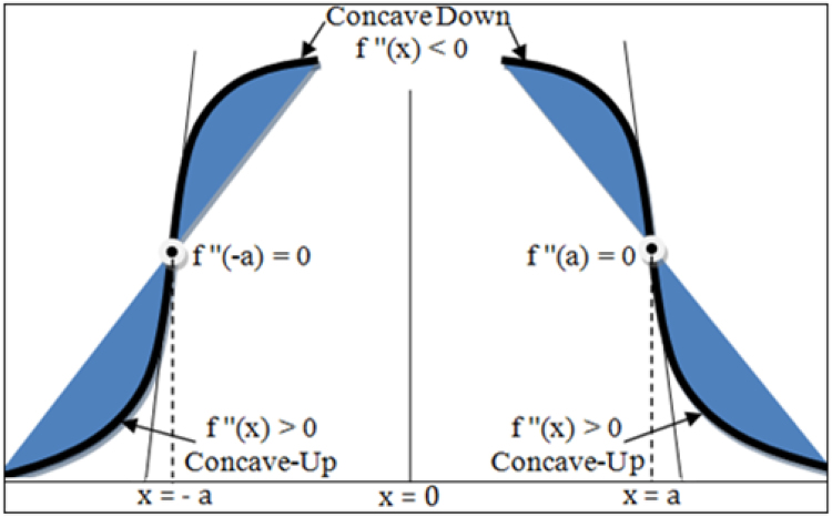
If function f′(x) changes from +Ve to −Ve values, we approach the local maxima. Similarly, if f′(x) changes from −Ve to +Ve values, we have local minima. Since at local minima and local maxima there exist f′′(x) = 0. Existence of f′′(x) = 0 is a necessary condition for the point of inflection at x, whereas f′′(x) = 0 and f′′′(x) ≠ 0 is a sufficient condition for the point of inflection to exist for a continuous function at point x. Fig. 1 illustrates how the concavities change around the inflection point.

Fig. 1.

Pictorial representation of change in concavity at points x = a and x = −a.

2.2. Manual procedures of inflection points

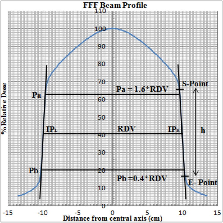
Removal of the flattening filter from the path of a photon beam changed the beam characteristics of FF beam and it became FFF beam with non-uniform fluence along the off-axis of the beam profile. In addition to the change of a dosimetric parameter of FFF beam, the change in the geometric shape of FFF beam was observed.¹¹ Because of the significant change in the shape of a beam profile, the conventional way of characterizing a flat beam profile cannot be applied to FFF beam. In order to analyze the characteristics of the FFF beam, the researcher came up with a concept of a point of inflection for the FFF beam. There are numerous works in literature proposing a theory about determining IPs for FFF beam. Rational of FFF beam profile can be explained with the help of the concept of IPs. IP is a property of the FFF beam profile and it can be determined by taking derivatives of the beam profile. This represents a variation of a dose along the off-axis. Researchers presented several mathematical methods of determining IPs such as extremum surface estimator (ESE) or extremum distance estimator (EDS), Newton, spline interpolation method.⁹ Analyzing characteristics of FFF beam profiles as per the definition of IPs needs a dedicated software. Atomic Energy Regulatory Board (AERB) of India has stated a graphical manual method of estimating IPs and analysis of FFF beam. AERB constituted a Task Group (TG) that involved experts from a regulatory agency.¹² We have used this method as a manual method of evaluating IPs for a FFF beam. Fig. 2 describes the graphical manual method of evaluating IPs and its characteristics. Manually IPs defined as the midpoint on either side of the high dose gradient region (sharply descending part) of the FFF beam profile.¹² In order to get the region of high dose gradient, start (S) and end (E) points are defined on either side of the beam profile. Height of the high dose gradient region (h) was identified as shown in Fig. 2. The point at h/2 is considered as a point of inflection. Dose value corresponds to h/2 (IPs) considered as a reference dose value (RDV). Field size is usually defined by the collimator setting at the isocenter. For a FFF beam, a radiological field is defined as the separation between left and right IPs. As per the AERB TG protocol for determining radiation beam penumbra, dose values at IP are taken as RDV. Points Pa and Pb, which are located at 1.6 and 0.4 times of RDV, respectively, are identified in Fig. 2. Lateral separation between those Pa and Pb on either side of the profile are defined as radiation beam penumbra.¹²

Fig. 2.

Schematic diagram for determining inflection point, field size and penumbra.

2.3. First principle of derivatives

The first principle of derivatives is a basic fundamental principle of derivatives. In 1823, Cauchy defined the derivatives of function f(x) in the form of a limit; when it exists, the quotient difference of (f(x + h) − f(x))/h goes to zero.¹³ Cauchy provided a proof called mean value theorem for derivative illustration. The theorem states that: if function f(x) is continuous on [x, x + h], then

$$\underset{[x,x+h]}{\min f^{\prime }(x)}\le \frac{f(x+h)-f(x)}{h}\le \underset{[x,x+h]}{\text{max}{f}^{\prime }(x)}$$ (4)

This principle itself referred to as postulates in mathematics, which cannot be derived from any other alternative postulates.

Let f(x) be a real value function and then its derivatives of function f(x) are defined as,¹⁴

$$f^{\prime }(x)=\underset{h\to 0}{\lim }\left\{\frac{f(x+h)-f(x)}{h}\right\}\text{R}.\text{H}.\text{Limit}$$ (5)

$$f^{\prime }(x)=\underset{h\to 0}{\text{lim}}\left\{\frac{f(x+h)-f(x)}{-h}\right\}\text{L}.\text{H}.\text{Limit}$$ (6)

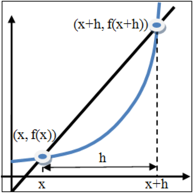
Fig. 3 can explain the physical interpretation of the first principle of derivatives.¹³ Method involved considering quotient of a difference of the value of a function at a different location to the increment h computing slope of the secant.

$$\frac{f(x+h)-f(x)}{h}$$ (7)

Fig. 3.

Pictorial representation of the first principle of derivative.

Fig. 3 indicates that, when quantity h vanishes, secant becomes tangent. Therefore neglecting h in the expression for the slope, Eq. (7) of the secant gives the slope of the tangent.

According to the definition of an inflection point, to ensure a change in concavity, the second derivative needs to be determined. The second derivative was derived from differentiating the first derivative as follows:

$$\begin{array}{lll}{f}^{″}(x)\hfill & =\frac{d}{dx}\{f^{\prime }(x)\}\hfill & =\frac{d}{dx}\left(\underset{h\to 0}{\text{lim}}\frac{f(x+h)-f(x)}{h}\right)\hfill \\ \hfill & \hfill & =\underset{h\to 0}{\text{lim}}\left(\frac{f^{\prime }(x+h)-f^{\prime }(x)}{h}\right)\hfill \\ \hfill & f^{″}(x)\hfill & =\underset{h\to 0}{\text{lim}}\left(\frac{f(x+2h)-2f(x+h)+f(x)}{h^2}\right)\hfill \end{array}$$ (8)

2.4. Python programming

Python was invented by Guido Rossum in the late 1980s. It is a powerful high-level interpreted, object-oriented and scripting programming language with dynamic semantics. Python has many application domains, such as a website, internet, and software development. Furthermore, it has been utilized in education, desktop GUIs, scientific numeric computing and scientific simulation programming. Similarly, for scientific programming, it has been practiced in simulating bimolecular, collaborative drug discovery, meteorologistic, energy efficiency, weather forecasting and many more.¹⁵ Each programming language has its unique advantage. However, python can be more user friendly because of its more intuitive coding style. We have developed the python code to find IPs of a FFF beam and its associate dosimetric parameters. For that, we employed free open source Python software of Pycharm Community Edition 2017.2.4 version. Entire Python code consists of several parts in the order. It comprises a code for importing Python module, selecting user beam profile data in text format via opening dialog box automatically and calculating the first and second derivatives based on the mathematical first principle of derivatives. To understand the change of concavity around the point of inflection, python code programming was developed to plot the graph. Following that, the code was extended to find IPs and IP dependent dosimetric beam parameters on both sides of the beam profile. Finally, the codes were compiled to plot the graph and display results. Python code for this program is as follows.

##### Importing module ########################

import numpy as np

import pandas as pd

import matplotlib.pyplot as plt

from tkinter import*

from tkinter import filedialog

##### Importing user data ######################

root = Tk()

Profile = filedialog.askopenfile()

user_cols = [“Distance”, “Dose”]

df1 = pd.read_table(Profile, names=user_cols, header=None)

#####Define 1st and 2nd derivative with central divide difference using superposition principle -function

h = (df1.ix[1,“Distance”] - df1.ix[0,“Distance”])

X = df1[“Distance”]

Y = df1[“Dose”]

def f1():

f1 = (((df1.ix[count + 1, “Dose”]) - (df1.ix[count - 1, “Dose”])) / (2 * h))

return f1

def f2():

f2 = (((df1.ix[count + 2, “Dose”]) - 2*(df1.ix[count, “Dose”]) + (df1.ix[count - 2, “Dose”])) / (4 * h * h))

return f2

##### Calculation first and second derivatives #####

X1 = df1.iloc[1:len(X)-1,0]

X2 = df1.iloc[2:len(X)-2,0]

Y1 = []

Y2 = []

for i in df1[“Dose”]:

count = 1

while count <= (len(Y)-2):

f1_store = Y1.append(f1())

count += 1

count = 2

while count <= (len(Y)-3):

f2_store = Y2.append(f2())

count += 1

break

df2 = pd.DataFrame(list(zip(Y1, Y2)), columns = [“f’(x)”, “f”(x)”])

Data = pd.concat([df1, df2], axis = 1)

###### Finding the Beam Profile parameters ######

## Inflection Points

Rt_maxslope = int(Y1.index(max(Y1)))

Rt_ipvalues = Y2[(Rt_maxslope-6):(Rt_maxslope+4)]

Rt_disvalue = X[(Rt_maxslope-4):(Rt_maxslope+6)]

Rt_dosevalue = list(Y[(Rt_maxslope-4):(Rt_maxslope+6)])

RtSign_Change = int(np.where(np.diff(np.sign(Rt_ipvalues)))[0])

Lt_minslope = int(Y1.index(min(Y1)))

Lt_ipvalues = Y2[(Lt_minslope-5):(Lt_minslope+5)]

Lt_disvalue = X[(Lt_minslope-3):(Lt_minslope+7)]

Lt_dosevalue = list(Y[(Lt_minslope-3):(Lt_minslope+7)])

LtSign_Change = int(np.where(np.diff(np.sign(Lt_ipvalues)))[0])

RtIP_df = pd.DataFrame(list(zip(Rt_disvalue, Rt_dosevalue, Rt_ipvalues)), columns = [“Rt_dis”, “Rt_dose”, “f”(x)”])

LtIP_df = pd.DataFrame(list(zip(Lt_disvalue, Lt_dosevalue, Lt_ipvalues)), columns = [“Lt_dis”, “Lt_dose”, “f”(x)”])

Rt_RDV = (RtIP_df.ix[RtSign_Change, “Rt_dose”] + RtIP_df.ix[RtSign_Change+1, “Rt_dose”])/2

Lt_RDV = (LtIP_df.ix[LtSign_Change, “Lt_dose”] + LtIP_df.ix[LtSign_Change+1, “Lt_dose”])/2

RDV = ((Rt_RDV)+ (Lt_RDV))/2

## Field Size

Rt_Fwidth = (RtIP_df.ix[RtSign_Change, “Rt_dis”] + RtIP_df.ix[RtSign_Change+1, “Rt_dis”])/2

Lt_Fwidth = (LtIP_df.ix[LtSign_Change, “Lt_dis”] + LtIP_df.ix[LtSign_Change+1, “Lt_dis”])/2

Field_Width = (Lt_Fwidth - Rt_Fwidth)

Field_Size = Field_Width/10

## Beam Penumbra

ZeroPoint = int(df1[df1[“Distance”] = = 0].index.values.astype(int))

Rt_X = X[0:ZeroPoint+1]

Rt_Y = Y[0:ZeroPoint+1]

Rt_df = pd.DataFrame(list(zip(Rt_X, Rt_Y)), columns=[“Rt_X”, “Rt_Y”])

Rt_Pa = 1.6*Rt_RDV

Rt_Pb = 0.4*Rt_RDV

Lt_X = X[ZeroPoint:len(X)]

Lt_Y = Y[ZeroPoint:len(X)]

Lt_df = pd.DataFrame(list(zip(Lt_X, Lt_Y)), columns=[“Lt_X”, “Lt_Y”])

Lt_Pa = 1.6*Lt_RDV

Lt_Pb = 0.4*Lt_RDV

pa = []

pb = []

for value in Rt_Y:

if value >= Rt_Pa:

pa = Rt_df[Rt_df[“Rt_Y”] = = value].index.values.astype(int)

break

for value in Rt_Y:

if value >= Rt_Pb:

pb = Rt_df[Rt_df[“Rt_Y”] = = value].index.values.astype(int)

break

pa_Rt = (Rt_df.ix[int(pa), “Rt_X”] + Rt_df.ix[int(pa-1), “Rt_X”])/2

pb_Rt = (Rt_df.ix[int(pb), “Rt_X”] + Rt_df.ix[int(pb-1), “Rt_X”])/2

Rt_penumbra = (pb_Rt - pa_Rt)

for value in Lt_Y:

if value <= Lt_Pa:

pa = Lt_df[Lt_df[“Lt_Y”] = = value].index.values.astype(int)

break

for value in Lt_Y:

if value <= Lt_Pb:

pb = Lt_df[Lt_df[“Lt_Y”] = = value].index.values.astype(int)

break

pa_Lt = (Lt_df.ix[int(pa-1), “Lt_X”] + Lt_df.ix[int(pa), “Lt_X”])/2

pb_Lt = (Lt_df.ix[int(pb-1), “Lt_X”] + Lt_df.ix[int(pb), “Lt_X”])/2

Lt_penumbra = (pb_Lt - pa_Lt)

print(Data)

print(“Right IP=”, Rt_RDV)

print(“Left IP=”, Lt_RDV)

print(“Average RDV=”, RDV)

print(“Field Size=”, Field_Size, “cm”)

print(“Rt Penumbra=”, Rt_penumbra, “mm”)

print(“Lt Penumbra=”, Lt_penumbra, “mm”)

###### Plotting Graph ###########################

fig = plt.figure()

graph = fig.add_subplot(1, 1, 1)

graph.spines[’left’].set_position((’data’, 0.0))

graph.set_xlim(-150, 150)

graph.set_ylim(-5, 100)

major_xticks = np.arange(-150, 150, 10)

major_yticks = np.arange(-5, 105, 5)

minor_xticks = np.arange(-150, 150, 1)

minor_yticks = np.arange(-5, 105, 1)

graph.set_xticks(major_xticks)

graph.set_xticks(minor_xticks, minor=True)

graph.set_yticks(major_yticks)

graph.set_yticks(minor_yticks, minor=True)

plt.grid(b=True, which=’major’, color=’black’, linestyle=’-’)

plt.grid(b=True, which=’minor’, color=’red’, linestyle=’-’)

plt.plot(X, Y, label=“Beam Profile”, color=“blue”, linewidth=0.5, marker=“*”, ms=1)

plt.plot(X2, Y2, label=“Inflection Points”, color=“black”, linewidth=0.5, marker=“*”, ms=1)

plt.xlabel(“Distance from central axis (cm)”)

plt.ylabel(“% Relative Dose”)

plt.title(Profile.name)

plt.legend()

plt.show()

root.mainloop()

####################### End of program code ##########################

3. Results

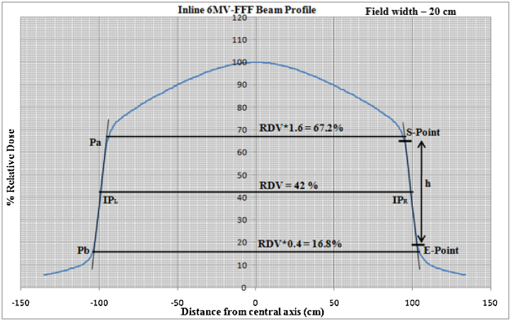
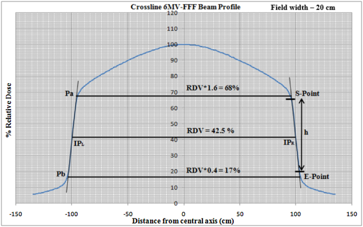
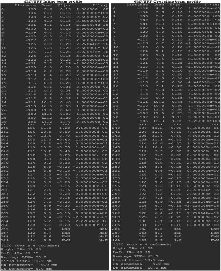
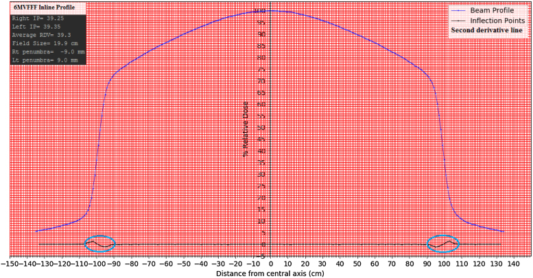
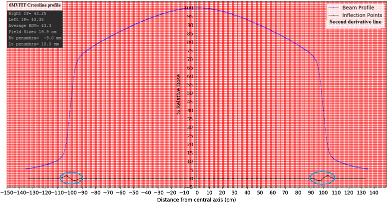
The graphical representations to determine an inflection point by the graphical manual method are shown in Fig. 4, Fig. 5. These figures further illustrate the determination of the beam characteristic parameter for 6MVFFF inline and crossline beam profiles. Then, the parameters, like dosimetric field size and beam penumbra, are determined manually. In another method of python code programming, the resulting output comprises values of the first and second derivatives based on the mathematical first principle of derivative and beam characteristics parameters are shown in Fig. 6. Resultant graphs with a line of concavity (line of second derivatives) indicating the point of inflection are shown in Fig. 7, Fig. 8. Table 1 summarizes the estimated results for both methods.

Fig. 4.

Schematic diagram describing the 6MVFFF inline beam profile for determining an inflection point, field size and penumbra by graphical manual method.

Fig. 5.

Schematic diagram describing the 6MVFFF crossline beam profile for determining an inflection point, field size and penumbra by graphical manual method.

Fig. 6.

Resultant output after executing python code programming for the 6MVFFF inline and crossline beam profile.

Fig. 7.

Schematic diagram for the 6MVFFF inline beam profile for determining an inflection point, field size and penumbra by python code programming. Circle inscribed on the second derivative plot line are shoving the change of concavity that corresponds to the inflection point on either side of the profile.

Fig. 8.

Schematic diagram for the 6MVFFF crossline beam profile for determining an inflection point, field size and penumbra by python code programming. Circle inscribed on the second derivative plot line are shoving the change of concavity that corresponds to the inflection point on either side of the profile.

Table 1.

Inflection point and beam characteristics parameter determined with graphical manual method and python code programming.

Method of determination	6MVFFF
	Inline Beam Profile				Crossline Beam Profile
	Inflection point (%)	Field width (cm)	Right penumbra (Pa-Pb) (mm)	Left penumbra (Pa-Pb) (mm)	Inflection point (%)	Field width (cm)	Right penumbra (Pa-Pb) (mm)	Left penumbra (Pa-Pb) (mm)
Graphical manual method	42.0	19.81	9.9	10.4	42.5	19.92	9.50	9.30
Python programming	39.3	19.90	9.0	9.0	43.3	19.90	9.0	10.0
Difference	2.70	0.09	0.9	1.40	0.80	0.02	0.50	1.30

IPs determined by the graphical manual method and the mathematical first principle of derivatives in python programming for 6MVFFF inline beam profile are found at RDV 42% and 39.3%, respectively. Similarly, for the 6MVFFF crossline beam profile the values are found at RDV 42.5% and 43.3%, respectively. The percentage difference between the IPs determined by both methods for the 6MVFFF inline and 6MVFFF crossline beam profile are found to be 2.7% and 0.8%, respectively. While the penumbra difference between both methods on the right and left side of the 6MVFFF inline beam profile are found to be 0.9 mm and 1.4 mm, respectively. Similarly, for the 6MVFFF crossline beam profile the difference in penumbra is found 0.5 mm and 1.3 mm, respectively. Dosimetric field width for a FFF beam was determined by both methods. Estimated dosimetric geometric field width for the inline beam profile with the graphical manual method and python code programming are found to be 19.81 cm and 19.9 cm, respectively. Likewise, for the crossline beam profile, the values are found to be 19.92 cm and 19.9 cm, respectively. Field width variations between both methods are found to be minimal.

4. Discussion

Conventional radiotherapy has been practiced with a FF beam for many years. However, the significance of a flattened beam has diminished over time due to the technological advancement. Intensity modulations with segmented and dynamic motion of MLC are invented in the modern era. This brought a change in custom of radiation delivery. This kind of delivery technique does not need a flattened beam specifically. In addition to that, there are well-established and proven clinical and dosimetric advantages of an unflattened or FFF beam over FF beam. Since the unflattened beam has been used predominantly in the treatment of high dose per fraction for SRS and SRT, dosimetric verification for small deviations in its beam characteristics parameters need to be evaluated periodically. However, conventional ways of analyzing FF beam do not hold good to FFF beam, so researchers came up with the concept of an inflection point.16, 17 Point of inflection has been used for analyzing beam characteristics of FFF beam. The inflection point is a point where the concavity changes and its second derivative exists absolute zero. Estimated inflection points with both methods are shown in Fig. 4, Fig. 5, Fig. 7, Fig. 8. Since the FFF beam is non-uniform along the width of the beam profile, IP is highly sensitive for a dose gradient. There is a large deviation in value of inflection points observed for a small change in the dose gradient. In graphical manual method, the degree of the dose gradient is determined from the trace of the tangent. However, the trace of the tangent cannot be drawn with high precision. Consequently, this could not allow us to determine exact IPs. Graphical manual method approximates the resulting values of IPs by extracting midpoint at h/2 in the dose gradient region are shown in Fig. 4, Fig. 5. Points of inflection differ with dose gradient, which is a function of beam energy, depth of measurement and field width¹⁸. In addition to that, trace of the tangent cannot account for small variation in the above parameters and IPs on either side of the beam profile are very much sensitive to beam symmetry. We have noticed that even a 1% symmetry deviation on either side of the beam profile can lead to a 2% of change in IPs. According to scientific literature, dosimetric field size defined for FFF beam is the separation between the IPs on either side of the beam profile. However, field width variations between both methods were found minimal. Even a change of 10% dose at the inflection point can influence the field width only by 1 mm.¹⁶ Second method of finding a point of inflection is based on a theoretical mathematical first principle of derivatives through python code programming. Theoretically, necessary and sufficient condition of inflection points is truly holds good for a continuous function. A beam spectrum of the linear accelerator is heterogeneous. Continuity in a beam profile cannot be maintained truly because of the fluctuation in beam energy fluence. First and second derivatives were estimated at every point of measurement at each step increment of 1 mm to find out the point where it satisfies the condition of IPs through developed python code programming. Fig. 6 shows the value of second derivatives describing concavity changes that correspond to IPs calculated by python code. We observed a concavity change occurring multiple times due to the fluctuation in the beam energy that was considered as noise. However, from the value of the second derivatives, we can see that the function is truly continuous near the point of inflection shown in Fig. 6. Concavity curve for IPs shown in Fig. 7, Fig. 8 shows how the IPs existed for concavity changes near the point of inflection for continuous functions. Concavity curve also shows the existence of maxima and minima near the point of inflection. Python code uniquely determined point of inflection between maxima and minima where the second derivatives goes zero. Therefore, the theoretical basis of determining an inflection point is independent of dose gradient, detector size, and measurement step size of the inflection point through python code programming was found to be reliable and consistent.

5. Conclusions

The graphical manual method of determining inflection point was found very cumbersome, tedious and there are many possibilities of human error. This method approximates the resultant value of IPs and it could not determine them precisely. Besides, this method could not account for a small change in the dose gradient, measurement step size and beam symmetry of the profile. Whereas, IPs determined based on the mathematical first principle of derivative through python code programming truly account for small changes in beam profile, measurement steps size and symmetry. This method was found highly effective to find out location of IPs independently and precisely on either side of beam profile. This was found to be more efficient, fastest and user-independent.

Conflicts of interest

None declared.

Financial disclosure

None declared.

References

- 1.Georg D., Knoos T., McClean B. Current status and future perspective of flattening filter free photon beams. Med Phys. 2011;38:1280–1293. doi: 10.1118/1.3554643. [DOI] [PubMed] [Google Scholar]
- 2.Titt U., Vassiliev O.N., Ponisch F. A flattening filter free photon treatment concept evaluation with Monte Carlo. Med Phys. 2006;33:1595–1602. doi: 10.1118/1.2198327. [DOI] [PubMed] [Google Scholar]
- 3.Vassiliev O.N., Titt U., Ponisch F. Dosimetric properties of photon beams from a flattening filter free clinical accelerator. Phys Med Biol. 2006;51:1907–1917. doi: 10.1088/0031-9155/51/7/019. [DOI] [PubMed] [Google Scholar]
- 4.Fu W., Dai J. Delivery time comparison for intensity modulated radiation therapy with/without flattening filter: a planning study. Phys Med Biol. 2004;49:1535–1547. doi: 10.1088/0031-9155/49/8/011. [DOI] [PubMed] [Google Scholar]
- 5.Kragl G., af Wetterstedt S., Knausl B. Dosimetric characteristics of 6 and 10 MV unflattened photon beams. Radiother Oncol. 2009;93:141–146. doi: 10.1016/j.radonc.2009.06.008. [DOI] [PubMed] [Google Scholar]
- 6.Vassiliev O.N., Kry S.F., Kuban D.A. Treatment planning study of prostate cancer intensity-modulated radiotherapy with a Varian Clinac operated without a flattening filter. Int J Radiat Oncol Biol Phys. 2007;68:1567–1571. doi: 10.1016/j.ijrobp.2007.04.025. [DOI] [PubMed] [Google Scholar]
- 7.Hrbacek J., Lang S., Klock S. Commissioning of photon beams of a flattening filter-free linear accelerator and the accuracy of beam modeling using an anisotropic analytical algorithm. Int J Radiat Oncol Biol Phys. 2011;80:1228–1237. doi: 10.1016/j.ijrobp.2010.09.050. [DOI] [PubMed] [Google Scholar]
- 8.Hrbacek J., Lang S., Graydon S.N. Dosimetric comparison of flattened and unflattened beams for stereotactic ablative radiotherapy of stage I non-small cell lung cancer. Med Phys. 2014;41:031709. doi: 10.1118/1.4866231. [DOI] [PubMed] [Google Scholar]
- 9.ChristopoulosF D.T. On the efficient identification of an inflection point. Int J Math Scientific Comput. 2016;6:1. [Google Scholar]
- 10.Goshu A.T., Koya P.R. Derivation of inflection points of nonlinear regression curves – implications to statistics. Am J Theor Appl Stat. 2013;2(6):268–272. [Google Scholar]
- 11.Cashmore J. The characterization of unflattened photon beams from a 6 MV linear accelerator. Phys Med Biol. 2008;53:1933–1946. doi: 10.1088/0031-9155/53/7/009. [DOI] [PubMed] [Google Scholar]
- 12.Sahani G., Sharma S.D., Sharma P.K., Deshpande D.D. Acceptance criteria for flattening filter-free photon beam from standard medical electron linear accelerator: AERB task group recommendations. J Med Phys. 2014;39:206–211. doi: 10.4103/0971-6203.144482. [DOI] [PMC free article] [PubMed] [Google Scholar]
- 13.Jadith V., Grabiner The changing concept of change: the derivative from Fermat to Weierstrass. Math Assoc Am. 1989;56:195–206. [Google Scholar]
- 14.Lim K.F. Differentiation from first principles using spreadsheets. Aust Senior Math J. 2008;22:41–48. [Google Scholar]
- 15.Bogdanchikov A., Zhaparav M., Suliyev R. Python to learn programming. J Phys: Conf Ser. 2013;423:012027. [Google Scholar]
- 16.Ponisch F., Titt U., Vassiliev O.N. Properties of unflattened photon beams shaped by a multileaf collimator. Med Phys. 2006;33:1738–1746. doi: 10.1118/1.2201149. [DOI] [PubMed] [Google Scholar]
- 17.Fogliata A., Garcia R., Knoos T. Definition of parameters for quality assurance of flattening filter free (FFF) photon beams in radiation therapy. Med Phys. 2012;39:6455–6464. doi: 10.1118/1.4754799. [DOI] [PubMed] [Google Scholar]
- 18.Muralidhar K.R. Derivation of equations to define inflection point and its analysis in flattening filter free photon beams based on the principle of polynomial function. Int J Canc Ther Oncol. 2015;3:1. [Google Scholar]