Dynamic Spectrotemporal Feature Selectivity in the Auditory Midbrain

Abstract

The transformation of auditory information from the cochlea to the cortex is a highly nonlinear process. Studies using tone stimuli have revealed that changes in even the most basic parameters of the auditory stimulus can alter neural response properties; for example, a change in stimulus intensity can cause a shift in a neuron's preferred frequency. However, it is not yet clear how such nonlinearities contribute to the processing of spectrotemporal features in complex sounds. Here, we use spectrotemporal receptive fields (STRFs) to characterize the effects of stimulus intensity on feature selectivity in the mammalian inferior colliculus (IC). At low intensities, we find that STRFs are relatively simple, typically consisting of a single excitatory region, indicating that the neural response is simply a reflection of the stimulus amplitude at the preferred frequency. In contrast, we find that STRFs at high intensities typically consist of a combination of an excitatory region and one or more inhibitory regions, often in a spectrotemporally inseparable arrangement, indicating selectivity for complex auditory features. We show that a linear–nonlinear model with the appropriate STRF can predict neural responses to stimuli with a fixed intensity, and we demonstrate that a simple extension of the model with an intensity-dependent STRF can predict responses to stimuli with varying intensity. These results illustrate the complexity of auditory feature selectivity in the IC, but also provide encouraging evidence that the prediction of nonlinear responses to complex stimuli is a tractable problem.

Introduction

The inferior colliculus (IC) in the mammalian midbrain serves as integrative center in the ascending auditory pathway where inputs from numerous peripheral areas are combined for transmission to the thalamus and cortex. The integration of spectral and temporal information in the IC is a highly nonlinear process, with the response properties of individual neurons changing dramatically under different stimulus conditions. For example, studies using pure tone and amplitude modulated tone stimuli have revealed that changes in stimulus intensity can evoke changes in both spectral (preferred frequency and bandwidth) and temporal (preferred modulation frequency and bandwidth) processing (Krishna and Semple, 2000; Frisina, 2001; Escabi and Read, 2005). Although responses to tone stimuli have provided the foundation for our current understanding of the IC, attempts to relate responses to tone stimuli and responses to more complex stimuli have revealed additional complexities (Ehret and Merzenich, 1988; Klug et al., 2002; Holmstrom et al., 2007). Thus, to understand how the nonlinear response properties of IC neurons effect the processing of complex stimuli, responses to such stimuli must be investigated directly.

In this study, we characterize the effects of stimulus intensity on selectivity for spectrotemporal features in responses to complex stimuli in the IC. Our analysis is based on the spectrotemporal receptive field (STRF), which is the linear filter that best describes the relationship between the auditory stimulus (in spectrogram form) and the neural response (Aertsen and Johannesma, 1981; Escabi and Read, 2003). Although the STRF is intended for use with linear systems, it can also be used to characterize response properties in systems with certain nonlinearities (Escabi and Read, 2003; Schwartz et al., 2006). Although auditory midbrain responses are generally highly nonlinear, they are in fact well described by an STRF (in combination with a static nonlinearity) at steady state, i.e., when the statistical properties of the stimulus are not changing (Eggermont et al., 1983; Escabi and Schreiner, 2002; Woolley et al., 2006). Thus, for a given stimulus, the STRF provides an accurate characterization of the feature selectivity of a neuron, and the effects of stimulus-dependent nonlinearities on feature selectivity can be investigated by comparing STRFs measured from responses to different stimuli (for a linear system, STRFs measured from responses to all stimuli would be identical). This approach has been used to identify potential nonlinearities in the responses of auditory neurons in various species to different types of auditory stimuli (i.e., vocalizations and random noise) (Eggermont et al., 1983; Theunissen et al., 2000; Blake and Merzenich, 2002; Escabi and Schreiner, 2002; Woolley et al., 2006), although the results of a recent study suggest that some of the differences in STRFs observed in these studies may not actually reflect stimulus-dependent nonlinearities, but rather the effects of higher-order stimulus correlations on the STRF estimate (Christianson et al., 2008).

To characterize the effects of stimulus intensity on selectivity for spectrotemporal features, we measure STRFs from IC responses to complex stimuli at different intensities. We find that feature selectivity is strongly dependent on stimulus intensity, with the complexity of the preferred features increasing as stimulus intensity increases. However, we also demonstrate that despite the complex effects of stimulus intensity on IC responses properties, responses to stimuli with varying intensity can be predicted by a relatively simple model. Together, these results provide a comprehensive phenomenological and functional description of intensity-dependent nonlinear processing of complex stimuli in the IC.

Materials and Methods

Physiological recordings.

The surgical procedures used in this study have been described in detail previously (Siveke et al., 2006). All experiments were approved according to the German Tierschutzgesetz (AZ 211-2531-40/01 and AZ 211-2531-68/03). Briefly, adult Mongolian gerbils (Meriones unguiculatus) were anesthetized for surgery with an initial intraperitoneal injection (0.5 ml/100 g body weight) of a physiological NaCl solution containing ketamine (20%) and xylazine (2%). During recordings, a dose of 0.03 ml of the same mixture was applied subcutaneously every 20 min. A small metal rod was mounted on the frontal part of the skull and used to secure the head of the animal in a stereotactic device during recordings. The animal was positioned in a sound-attenuated chamber and a craniotomy was made over the inferior colliculus, 1.3–2.6 mm lateral from the midline and 0.5–0.8 mm caudal from the bregma. The dura mater overlying the cortex was removed, and glass electrodes filled with 1 m NaCl (5–15 MΩ) were advanced into the inferior colliculus (2–4 mm below the surface).

Extracellular action potentials were recorded, filtered, and fed into a computer via an analog-to-digital converter (RP2–1; Tucker-Davis Technologies). Only recordings with high signal-to-noise ratio (>5) and stable spike waveforms were retained. Clear isolation of action potentials from single-units was achieved by off-line spike cluster analysis (Brainware; Jan Schnupp, Tucker-Davis Technologies). Typical recording periods lasted 10–14 h. After recordings, the animal was killed without awakening by an injection of 0.1 ml of barbital. For some animals, the last electrode position was marked by a pressure-induced injection of Dextran and recording sites were verified to be in the central nucleus of the inferior colliculus using standard histological techniques (Siveke et al., 2006).

Acoustic stimulation.

Stimuli were generated with a 48 kHz sampling rate by TDT System III hardware (Tucker-Davis Technologies). Digitally generated stimuli were converted to analog signals (RP2–1), attenuated (PA5), and delivered to an electrostatic speaker (EC1) coupled to a tube which was inserted in the ear canal. All stimuli were presented monaurally to the ear contralateral to the recording site. Speakers were calibrated to have a flat frequency response [±5 dB sound pressure level (SPL) from 0.4–20 kHz, frequencies outside this range were not presented] and the frequency spectrum of the rain stimulus (described below) recorded from the end of the tube matched that of the original recording used to generate the stimulus, indicating that the stimulus was presented without distortion. For pure tones, the total harmonic distortion (ratio of power at all harmonics to power at fundamental) was 3% at 97 dB SPL. When searching for neurons, repeated presentations of a 200 ms segment of broadband noise were presented. When the response of a single neuron was isolated, 200 ms pure tones of various intensities and frequencies were presented to determine the frequency-response area (FRA) (see Fig. 1j). Only those neurons with sustained responses to the pure tone stimulus (those that responded on average with more than one spike in the last 150 ms of a 200 ms stimulus at the preferred frequency, 20 dB SPL above threshold) were included in this study.

Figure 1.

The STRFs of neurons in the inferior colliculus vary with stimulus intensity. a, The sound pressure distribution of the rain stimulus. The pressure signal was normalized to have a maximum value of 1 and a minimum value of −1. b, The spectrogram of a 400 ms segment of the stimulus. The spectrogram was computed with frequency bins spaced at one-tenth octave, time bins spaced at 2 ms, and a 4 ms hamming window. The colors denote the intensity of the stimulus in dB SPL. c, The frequency spectrum of the stimulus in dB SPL, averaged across a 40 s segment. d, The modulation spectrum of the stimulus. The modulation spectrum was obtained by computing the power spectrum of the amplitude modulations within each frequency bin of the spectrogram (after normalizing the amplitude modulations to have a maximum value of 1) and averaging the results across all frequency bins. e, The responses of a typical IC neuron to 50 repeats of a 500 ms segment of the rain stimulus at three intensities: 52, 72, and 92 dB SPL. Inset, The segments surrounding threshold crossings in the extracellular recording of this response that were classified as either spikes (red) or noise (black). f, The RLF relating mean firing rate to the intensity of the rain stimulus for the neuron for which responses are shown in e. The intensities corresponding to the responses in e are marked with colored boxes. g, h, The responses and rate-level function for a second neuron, displayed as in e and f. i, A schematic diagram of a linear–nonlinear (LN) model describing the mapping from stimulus to response in the inferior colliculus. The auditory stimulus in spectrogram form (s) is passed through the STRF (summation across frequency, convolution across time) to produce the intermediate signal y, which reflects the stimulus-related modulations in the membrane potential of the neuron. The intermediate signal is passed through the static NL to yield a time-varying firing rate (r). For more details, see Materials and Methods. j, The FRA relating mean firing rate to the intensity of a pure tone stimulus for the neuron for which responses are shown in e. k, The STRFs measured from responses to a 40 s segment of the rain stimulus (the training stimulus) at 52, 72, and 92 dB SPL for the neuron for which responses are shown in b. Red and blue areas indicate excitatory and inhibitory regions according to the color bar. The units of the STRF are arbitrary (but proportional to hertz per decibel). STRFs were smoothed with a 3 × 3 pixel Gaussian window for plotting. l, The NLs measured from responses to the rain stimulus at 52, 72, and 92 dB SPL for the neuron for which responses are shown in b. Colors correspond to the intensity of the stimulus. The horizontal axis corresponds to the result of passing the stimulus through the STRF, after normalization to unit variance. m–o, The FRA, STRFs, and NLs for the neuron for which responses are shown in g, displayed as in j–l.

The main stimulus used in this study was the sound of rain (obtained from the Freesound Project, Universitat Pompeu Fabra, Barcelona, Spain). The statistical properties of this stimulus are shown in Figure 1a–d, and a file containing a short segment of the stimulus is provided in the supplemental material (available at www.jneurosci.org). For all neurons (n = 40), a 10 s segment of the rain stimulus was presented at range of intensities to determine a rate-level function (RLF) (see Fig. 1f). Then, the “training” stimulus, 10 repetitions of a 40 s segment, was presented at two intensities: the intensity that evoked the maximum firing rate (“high SPL”), and a lower intensity that evoked a firing rate that was at most half of the maximum (“low SPL”). The responses to these stimuli were used for calculation of the STRFs and nonlinearities (NLs) as described below. Next, the “testing” stimulus, 50 repetitions of a 5 s segment of the rain stimulus different from that used in the training stimulus, was presented at the same two intensities. The responses to this stimulus were used to test the predictive power of the linear–nonlinear model as described below. Although the training and testing stimuli were drawn from separate segments of the original sound recording, their statistical properties were indistinguishable. For a subset of neurons, we also presented other stimuli including the training stimulus at other intensities and a second testing stimulus, 50 repetitions of a 10 s segment of stimulus in which, within each repetition, the intensity was systematically varied between 57 and 97 dB SPL (see Fig. 3). All repetitions of a given stimulus were presented contiguously (i.e., with no pause between repetitions). For all analyses, responses to the first 10 s of each contiguous block of stimuli were ignored. No artificial rise/fall time was imposed on the stimulus.

Figure 3.

Predicting responses of neurons in the inferior colliculus to stimuli with different intensities. a, The high- and low-intensity STRFs and NLs for a typical cell (92 and 77 dB). b, The actual responses (black) of the neuron for which the STRFs and NLs are shown in a to the same 350 ms segment of stimulus at low and high intensity (PSTH, averaged across 50 repetitions), along with the predicted responses (blue) of the linear–nonlinear model with the matched STRF and NL (i.e., the low-intensity STRF and NL were used to predict the response to the low-intensity stimulus and the high-intensity STRF and NL were used to predict the response to the high-intensity stimulus). The correlation coefficients (for firing rate in 2 ms bins) between the predicted and actual responses are indicated. Correlation coefficients were calculated for the entire response to the 5 s testing stimulus. c, The same actual responses as in b, along with the predicted responses of the linear–nonlinear model with the switched STRF and NL (i.e., the high-intensity STRF and NL were used to predict the response to the low-intensity stimulus and vice versa). d, The mean correlation coefficients between the actual and predicted responses for the matched and switched linear–nonlinear models, along with models in which only the STRF or the NL were switched, for a population of 40 neurons. Error bars indicate 1 SD. e, A schematic diagram of an extended LN model with intensity-dependent STRF and NL. At each time step, the current intensity of the stimulus was used to determine the appropriate shapes STRF and NL. f, The STRFs and NLs measured from responses to the rain stimulus at three intensities for two neurons that displayed strong intensity-dependent nonlinearities. g, The intensity of a 10 s segment of rain stimulus in which intensity was increased and decreased logarithmically between 57 and 97 dB SPL. h, The correlation coefficients between the actual and predicted responses to a 10 s segment of the rain stimulus with varying intensity as shown in g for the intensity-dependent linear–nonlinear model (cyan) and models with either the high- (black) or low-intensity (red) STRFs and NLs for the two neurons for which STRFs and NLs are shown in f. Correlation coefficients were calculated in 500 ms segments.

Linear–nonlinear model of auditory processing.

The transformation from stimulus to response in the early auditory pathway can be represented by a linear–nonlinear cascade of a linear filter and a rectifying static nonlinearity (see Fig. 1i). The stimulus is defined as a spectrogram s[k,n] with zero mean and logarithmic amplitude that specifies the time-varying intensity at a range of carrier frequencies (calculation of spectrograms is described below). At each time step, to produce the intermediate signal y[n], which reflects the stimulus-related modulations in the membrane potential of the neuron, the stimulus is passed through the linear filter g[k,m] (summation in space, convolution in time) representing n_k (number of frequency bins in spectrogram) separate temporal filters each with n_m parameters. This linear filter is known as the STRF and reflects the spectral and temporal integration of the stimulus within the circuitry of the auditory pathway. The output of the STRF, y[n], is passed through a static nonlinearity f (.) to yield the non-negative firing rate r[n]. This static nonlinearity captures the transformation from the membrane potential of the neuron to its observed firing rate, and typically resembles a half-wave rectifier. Note that the spontaneous firing rate of the neuron is also reflected in the NL as a vertical offset.

The transformation from stimulus to response in the linear–nonlinear model at each time step can be written as a discrete-time summation:

or, for notational convenience, as a product of two vectors, r[n] = f (s_n^Tg), where s_n = [s[1,n], s[1,n − 1], …, s[1,n − n_m + 1],s[2,n], …, s[n_k,n − n_m+1]]^T and g = [g[1,1], g[1,2], …, g[1,n_m], g[2,1], …, g[n_k,n_m]]^T. For an entire stimulus/response record with n = 1, 2,…, N, the transformation from stimulus to response can be summarized as r = f (Sg), where r = [r[1], r[2], …, r[N]]^T and

To quantify the predictive power of an STRF and/or NL, we used the linear–nonlinear model to simulate neural responses and measured the correlation coefficient between these simulated responses and actual neural responses to the same stimulus (see Fig. 3). Correlation coefficients were corrected for finite data effects using the method described by David and Gallant (2005).

Calculation of spectrotemporal receptive fields.

STRFs were calculated via regularized least-squares estimation. The specific implementation of this procedure for the estimation of STRFs from auditory responses to complex sound stimuli has been described in detail previously (Machens et al., 2004). Here, we provide only a brief description of the procedure and indicate any parameter values that were specific to this study. First, the stimulus pressure waveform (sampled at 48 kHz) is converted to a zero-mean spectrogram by computing the discrete-time Fourier transform of successive overlapping windowed segments. In this study, each segment was 4 ms, the overlap between successive segments was 2 ms, and the segments were smoothed with a 4 ms Hamming window. This yielded a spectrogram with frequency bins with one-tenth octave spacing (after spectral resampling), and time bins with 2 ms spacing. Next, the time-varying firing rate of the neural response is computed with the same temporal resolution (and shifted to have zero mean) and the cross-covariance between the stimulus and response, A = S^Tr (S and r defined as above), and the auto-covariance of the stimulus, B = S^TS, are calculated for delays up to 40 ms (n_m = 20). Note that because of the high temporal resolution of the time-varying firing rate, A is approximately equivalent to computing the “spike-triggered average” by averaging together the 40 ms segments of spectrogram that preceded each spike in the response. In a standard least-squares estimation, the cross-covariance between the stimulus and response is divided by the auto-covariance of the stimulus to obtain the STRF, g = B⁻¹A. However, for natural stimuli, B may have many eigenvalues close to zero, and its inversion may introduce high-frequency noise into the STRF. To improve the STRF estimate, two regularization parameters are used: one that penalizes large deviations of the STRF from zero, and another that penalizes large differences between neighboring points in the STRF. The regularized STRF is given by g = (B + C)⁻¹A, with g defined as above and the elements of C given as follows:

where λ and μ are the regularization parameters, η_i is the set containing the neighboring points of the ith element of g (the neighboring points of the element of g corresponding to g[k,m] are the elements of g corresponding to g[k − 1,m], g[k + 1,m], g[k,m − 1], and g[k,m + 1]), |η_i| is the number of elements in η_i (this value is 4 for most points in the STRF, and lower for those points on the edge of the STRF with k = 1 or n_k, or m = 1 or n_m), and δ_ij is equal to one if i = j and zero otherwise.

To determine the optimal values of the regularization parameters, the 40 s training stimulus/response record was divided into segments of 36 and 4 s. The STRF was calculated for a range of parameter values (λ = 2ⁱ, μ = 2^j; with i, j = 0, 1, …, 10) using the stimulus and response corresponding to the 36 s segment. Each STRF was then used in the linear–nonlinear model to predict the response to the stimulus corresponding to the 4 s segment (after estimating the static nonlinearity as described below) and the mean squared error between the prediction and the actual response corresponding to the 4 s segment was computed. This process was repeated for 10 different permutations of the 36 and 4 s segments and those parameter values that yielded the lowest average prediction error were chosen as the optimal values. Note that only responses to the training stimulus were used in the calculation of the STRF.

To determine the significant points in the STRF, STRFs were also calculated (with the optimal regularization parameters) after the response (average time-varying firing rate, not individual spike trains) was randomized in time. The SD of this “shuffled” STRF was used as a measure of the noise in the original STRF. Significant points in the original STRF were defined as those that exceeded 3 SDs of the shuffled STRF. All nonsignificant regions in the original STRF were set to zero.

It should be noted that least-squares estimation provides an unbiased measurement of the STRF, independent of the strength of the second-order correlations in the stimulus. However, the rain stimulus used in this study also contains higher-order correlations. To ensure that these correlations did not introduce a bias into the STRF, we simulated responses to the rain stimulus with the measured high- and low-intensity STRFs for each neuron in this study (n = 40) using the standard linear–nonlinear model (with a half-wave rectifying static nonlinearity). Across the population, the mean difference between the STRFs calculated from these simulated responses and the actual STRFs was not significantly different from zero (t test, p < 0.01), indicating that, at least within the set of assumptions implied by the linear–nonlinear model, the higher-order correlations in the stimulus did not bias the measurement of the STRF. Furthermore, the fact STRFs derived from experimental responses to the training stimulus had high predictive power for responses to the testing stimulus of the same intensity (typical correlation coefficients between predicted and actual responses for firing rate in 2 ms time bins were between 0.5 and 0.6) suggests that these STRFs do indeed provide a good description of neural response properties for the stimuli used in this study.

Calculation of static nonlinearities.

The static NLs for each cell were calculated by convolving the stimulus spectrogram with the STRF to yield the intermediate signal y as described above, and comparing y to the actual firing rate of the neuron r. The scaling of the NL depends on the scaling of the corresponding STRF (for example, multiplying the STRF by 2 stretches the horizontal axis of the NL by a factor of 2). For this reason, to uniquely specify the STRF and NL, it is necessary to constrain the variance at some stage in the linear–nonlinear model. For the NLs presented in the Results, we constrained the output of the RF to have unit variance, allowing NLs for stimuli with different intensities to be compared on the same horizontal axis. For the results presented in Supplemental Figure 1 (available at www.jneurosci.org as supplemental material), we also constrained the variance of the output of the STRF to match that of the input to the STRF, effectively forcing all of the gain in the linear–nonlinear model into the NL.

To measure the static NL, the values of y were sorted into ascending order and separated into groups of 250 values. For each group, the mean values of y and the corresponding actual firing rates were used to define the static NL. When using the static NL in the linear–nonlinear model to predict neural responses, the firing rate for a particular value of y was determined by spline-based interpolation between points at which the NL was defined. For values of y that were outside the range of values for which the NL was defined, spline-based extrapolation was used.

Intensity-dependent linear–nonlinear model of auditory processing.

The standard linear–nonlinear model described above is intended to describe the response of neuron to a stationary stimulus (a stimulus in which the intensity is fixed) and, thus, the STRF g[k,m] and NL f (.) are time invariant. However, because auditory responses are nonlinear, an STRF and NL that provide good predictions of responses at one intensity I may not be suitable for stimuli with a different intensity I + ΔI. Thus, it is desirable to extend the model such that the STRF and NL are time-varying in a manner that depends on the current intensity of the stimulus [i.e., g[k,m] → g_I [k,m] and f (.) → f_I (.)]. To create such a model for a given neuron, we measured the STRF and NL at a series of intensities separated by ΔI; = 10 dB SPL. We then interpolated between the measured STRFs and NL to series of intensities separated by δI = 0.1 dB SPL to produce a large set of STRFs g_I [k,m] and NLs f_I (.) that varied with intensity. At each time step, the current intensity of the stimulus was used to choose the appropriate STRF and NL from this set to process the stimulus as described for the standard linear–nonlinear model.

Results

The preferred spectrotemporal features of neurons in the IC vary with stimulus intensity

We made extracellular single-unit recordings in the IC of anesthetized gerbils while presenting the sound of rain at different intensities. We chose this particular stimulus because of its spectrotemporal complexity and its ability to elicit strong and sustained responses from IC neurons. The sound pressure distribution of the stimulus (approximately Gaussian) is shown in Figure 1a, and the spectrogram of a one second segment of the stimulus is shown in Figure 1b. The overall power in the stimulus falls off with increasing carrier frequency, as shown in Figure 1c, whereas the power spectrum of the amplitude modulations is relatively flat, as shown in Figure 1d.

Figure 1e shows the responses of a typical neuron to repeated presentations of a 500 ms segment of the stimulus at 52, 72, and 92 dB SPL. The RLF of the neuron for the rain stimulus, displayed in Figure 1f, shows that the firing rate of the neuron increases with increasing intensity at low intensities before saturating at high intensities. The responses for a second neuron with an RLF that is monotonic (within the range of intensities that we tested) are shown in Figure 1, g and h.

We used the responses of these two neurons to 10 repetitions of a 40 s segment of the stimulus (the training stimulus) (see Materials and Methods) at several intensities to measure the parameters of a linear–nonlinear model. The linear–nonlinear model is a cascade of an STRF and a static nonlinearity, as shown in Figure 1i. The linear–nonlinear model can be used to simulate neural responses by passing the stimulus (in spectrogram form) through the STRF (summation across frequency, convolution across time) and then through the NL to produce a time-varying firing rate (for a full description, see Materials and Methods). Intuitively, the STRF can be viewed as a (time-reversed) spectrogram that reflects the preferred stimulus feature of the neuron, and the NL as a function that controls the gain of the model and ensures a positive firing rate. Thus, the firing rate of the model is determined by the degree to which the current stimulus matches the feature represented by the STRF.

As shown in Figure 1j, the FRA for the first neuron measured from responses to pure tones indicates that the neuron is responsive to frequencies between 0.4 and 6.4 kHz. The nonlinear response properties of this neuron are evident in the larger bandwidth of the FRA at higher intensities. This nonlinearity is also evident in the STRFs for this neuron at different intensities, shown in Figure 1k, which indicate that the neuron responds to a broader range of frequencies at higher intensities. However, the STRFs also illustrate the selectivity of the neuron for complex spectrotemporal features that are not evident in the FRA. At 52 dB SPL, the STRF consists of a single spectrotemporally narrow excitatory (red) region, indicating that the neural response is simply a reflection of the amplitude at the preferred frequency of 6 kHz. As the intensity is increased, the STRF becomes more complex, with a delayed inhibitory (blue) region at 6 kHz, as well as other excitatory and inhibitory regions at lower frequencies. These additional regions in the STRFs at higher intensities reflect the intensity-dependent nonlinearity in the neural response, and indicate the selectivity of the neural response for more complex features that are not evident in the FRA, such as spectral or temporal edges. The NLs for this neuron, shown in Figure 1l, reflect the saturating RLF shown in Figure 1f, with the smallest gain at 52 dB SPL (blue), and larger, similar gains at 72 and 92 dB SPL (red and green).

The FRA for the second neuron is shown in Figure 1m. The nonlinear response properties of this neuron are also evident in the FRA, as the preferred frequency shifts to lower frequencies as the intensity is increased. This shift is reflected in the excitatory regions of the STRFs, shown in Figure 1n, which also shift to lower frequencies as intensity is increased. The NLs for this neuron reflect the monotonic RLF shown in Figure 1 h, as gain increases with increasing intensity.

The preferred spectrotemporal features of neurons in the IC become more complex with increasing stimulus intensity

The results shown in Figure 1 illustrate that stimulus intensity can have dramatic effects on feature selectivity in the IC. To provide a systematic characterization of these effects, we compared STRFs at different intensities for a population of IC neurons (n = 40). Because the effects of intensity on NLs for auditory neurons have already been well documented (Nagel and Doupe, 2006), we focus our analysis on the STRFs only. However, for completeness, we also provide the results of our corresponding analysis of the NLs in Supplemental Figure 1 (available at www.jneurosci.org as supplemental material).

For each neuron, STRFs were measured from responses at two intensities: the intensity corresponding to the peak of the RLF (high SPL), and a lower intensity that evoked a firing rate that was at most half of the peak of the RLF (low SPL). The results for three typical cells are shown in Figure 2. For all three cells, the STRF at low intensity consisted of a single excitatory region, whereas the STRF at high intensity was more complex. For the first cell, an increase in intensity results in the emergence of a delayed inhibitory region at the preferred frequency. For the second cell, an increase in intensity results in the emergence of a delayed inhibitory region at the preferred frequency, as well a second inhibitory region above the preferred frequency, coincident with the excitatory region. For the third cell, an increase in intensity results in the emergence of an inhibitory region below the preferred frequency, coincident with the excitatory region, as well as delayed inhibitory and excitatory regions with different latencies.

Figure 2.

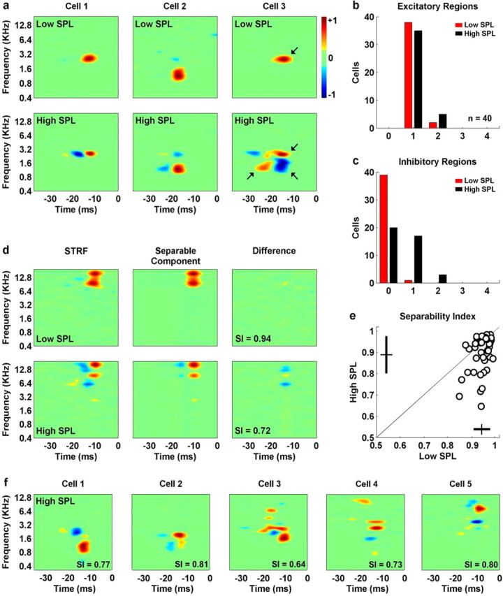
The STRFs of neurons in the inferior colliculus become more complex with increasing stimulus intensity. a, The STRFs for three cells measured from responses to the rain stimulus at two intensities (cell 1, 92 dB and 37 dB; cell 2, 72 dB and 32 dB; cell 3, 92 dB and 37 dB). The arrows on the STRFs for the third cell denote those regions whose strength (for definition, see Results) was large enough to be included in the counts shown in b and c. b, c, Histograms showing the number of excitatory and inhibitory regions in the low- (red) and high-intensity (black) STRFs for a population of 40 IC neurons. d, The high- and low-intensity STRFs for a typical neuron (97 and 72 dB), along with the separable component (the product of the functions of time and frequency corresponding to the largest singular value of the STRF) and the difference between the STRF and the separable component. The same color axes are used for the STRF, separable component, and difference plots. The separability index (the ratio of the largest singular value to the sum of all singular values) for each STRF is indicated. e, The separability indices of the high- and low-intensity STRFs for a population of 40 IC neurons. f, Five examples of high-intensity STRFs with low separability indices (cell 1, 92 dB; cell 2, 82 dB; cell 3, 92 dB; cell 4, 92 dB; cell 5, 92 dB).

To quantify the effects illustrated in Figure 2a, we counted the number of excitatory and inhibitory regions in the STRFs at high and low intensities. For a region to be included in the count, its strength had to be at least 25% of that of the strongest region in the same STRF (the strength of a region was defined as the absolute value of its integral). The regions that satisfied this criterion for the high- and low-intensity STRFs for the third cell in Figure 2a are indicated by arrows. As shown in Figure 2b, nearly all cells in the population had STRFs with a single excitatory region at both low (38 of 40) and high (35 of 40) intensities. The main difference between the high- and low-intensity STRFs was in the number of inhibitory regions, as shown in Figure 2c. Although only one cell had an STRF with an inhibitory region at low intensity, half of all cells (20 of 40) had STRFs that contained one or more inhibitory regions at high intensity.

To further characterize the complexity of the STRFs at high and low intensities, we determined the degree to which they were spectrotemporally separable, i.e., how well the STRFs can be described by the product of a single function of frequency and a single function of time. To quantify the spectrotemporal separability of an STRF, we computed its singular-value decomposition (Depireux et al., 2001; Sen et al., 2001; Escabi and Read, 2003) and computed the ratio of the first singular value to the sum of all the singular values. This quantity, termed the separability index (SI), is equal to one when the STRF is perfectly separable and decreases as the STRF becomes less separable.

The results for a typical neuron are shown in Figure 2d. At low intensity, the STRF for this neuron consists of single, vertically oriented excitatory region. This STRF is highly separable, with an SI of 0.94. This is reflected in the small difference between the actual STRF and the “separable component” (the STRF given by the product of the functions of frequency and time associated with the largest singular value). In contrast, the STRF for this neuron at high intensity consists of multiple excitatory and inhibitory regions with varying delay. The inseparability of this STRF (SI, 0.72) is reflected in the large difference between the actual STRF and the separable component. The decrease in separability at high intensity for this neuron was typical of the population, as illustrated in Figure 2e. Although no cells had an STRF with an SI <0.85 at low intensity, one quarter of all cells (10 of 40) had an STRF with an SI below this value at high intensities. The high-intensity STRFs for five of these cells are shown in Figure 2f, illustrating the range of complex spectrotemporal features for which IC neurons exhibit selectivity.

Predicting responses of neurons in the inferior colliculus to stimuli with different intensities

Our analysis assumes that the STRFs we measured at high and low intensities provide a valid description of a neuron's feature selectivity. If this is true, then an STRF measured at a given intensity should provide good predictions of the neural response to stimuli at that intensity. Furthermore, if the dramatic differences in STRFs at high and low intensity that we observe truly reflect changes in spectrotemporal feature selectivity, and this feature selectivity is an important response property, then an STRF measured at one intensity should provide poor predictions of the neural response to stimuli at different intensities.

To test the predictive power of our measured STRFs, we used the linear–nonlinear model to predict responses to high- and low-intensity stimuli and compared the predictions to actual responses. To ensure that the results of these tests were not influenced by “over fitting,” predictive power was measured for responses to a 5 s segment of the rain stimulus that was not used to measure the STRFs and NLs (the testing stimulus) (see Materials and Methods). The high- and low-intensity STRFs and NLs for a typical neuron are shown in Figure 3a. At low intensity, the STRF consists of two excitatory regions and an increase in intensity results in the emergence of additional inhibitory regions above the preferred frequency. The actual responses (black) of the neuron to the same 350 ms segment of stimulus at low and high intensity (PSTH, averaged across 50 repetitions) are shown in Figure 3b, along with the predicted responses (blue) of the linear–nonlinear model with the “matched” STRF and NL (i.e., the low-intensity STRF and NL were used to predict the response to the low-intensity stimulus and the high-intensity STRF and NL were used to predict the response to the high-intensity stimulus). The correlation coefficients (for firing rate in 2 ms time bins) between the predicted and actual responses were high (0.69 for low intensity, 0.59 for high intensity), indicating that the matched models have relatively high predictive power and that the STRFs are indeed a good description of the preferred stimulus features for this neuron. Figure 3c shows the same actual responses as Figure 3b, along with the predicted responses of the linear–nonlinear model with the “switched” STRF and NL (i.e., the high-intensity STRF and NL were used to predict the response to the low-intensity stimulus and vice versa). In this case, the correlation coefficients are much lower (0.42 for low intensity, 0.40 for high intensity), indicating that the switched models have relatively low predictive power and that the differences between the high- and low-intensity STRFs do indeed reflect changes in the response properties of this neuron.

We observed similar results across the population, as summarized in Figure 3d. On average, the correlation coefficients for the matched models (0.6 for low intensity, 0.52 for high intensity) were much higher than those for the switched models (0.31 for low intensity, 0.27 for high intensity), and these differences were highly significant (paired t tests, p < 0.001). To be sure that the differences in the predictive power of the matched and switched models were attributable to differences in the high- and low-intensity STRFs (and not to differences in NLs), we also predicted the neural responses after switching only the STRFs or NLs. As shown in Figure 6d, switching the NL had little effect on the predictive power of the model with the matched STRF, whereas switching only the STRF greatly reduced the predictive power of the model.

The intensity-dependent changes in STRFs (and NLs) that we observe indicate that the standard linear–nonlinear model is an incomplete description of IC response properties. However, given the success of the matched linear–nonlinear models at steady state, it is possible that an extended linear–nonlinear model such as the one illustrated in Figure 3e, with an STRF and NL that are intensity dependent, could predict responses to a stimulus with varying intensity. This extension effectively adds a second nonlinearity to the model that captures the intensity-dependent changes in the STRF and NL. Assuming the intensity-dependent changes in the STRF and NL are relatively smooth, we can construct such a model simply by estimating the STRFs and NLs from responses to stimuli at several different intensities, and interpolating between these measured results to determine the appropriate STRFs and NLs for intensities in between.

We tested this approach on two neurons that displayed strong intensity-dependent nonlinearities. We measured the STRFs and NLs for these neurons at five intensities between 57 dB SPL and 97 dB SPL at 10 dB SPL intervals. The STRFs and NLs for three of these intensities are shown in Figure 3f. An increase in intensity results in the emergence of two inhibitory regions in the STRF of the first neuron, and shifts the preferred frequency in the STRF of the second neuron. We tested the power of the extended linear–nonlinear model to predict the responses of these neurons to a 10 s segment of the rain stimulus (50 repetitions) in which the intensity increased logarithmically from 57 to 97 dB SPL over the first five seconds and returned to 57 dB SPL over the next 5 s, as illustrated in Figure 3g. At each time step, we simply interpolated between the measured STRFs and NLs to determine the appropriate STRF and NL for the current stimulus intensity (for example, the STRF used to predict the response to a 72 dB SPL stimulus would be a combination of the STRFs measured from responses to stimuli at 67 and 77 dB SPL).

The correlation coefficients for the extended linear–nonlinear model predictions, as well as those for the high-intensity and low-intensity linear–nonlinear models with fixed STRFs and NLs are shown in Figure 3h. For both neurons, the predictive power of the low-intensity model (red) is highest during the first and last segments of the stimulus, when the intensity of the stimulus is low, and lowest during the middle segment of the stimulus, when the intensity of the stimulus is high, whereas the predictive power of the high-intensity model (black) displays the opposite trend. For both neurons, the intensity-dependent model (cyan) is able to maintain high predictive power across the entire range of stimulus intensities. This result further demonstrates that the processing of a complex auditory stimulus at any particular intensity in the IC intensity is relatively linear, and suggests that nonlinear responses to complex stimuli can be described by an intensity-dependent linear–nonlinear model.

Discussion

The results of this study demonstrate intensity-dependent dynamic feature selectivity in the IC, beyond that which is apparent in responses to tone stimuli. Specifically, by comparing STRFs measured from responses to complex stimuli at different intensities, we observe a dramatic transition in the complexity of the preferred spectrotemporal features of individual neurons. At low intensities, STRFs typically consist of a single excitatory region, indicating that the neural response is simply a reflection of the stimulus intensity at the preferred frequency. In contrast, at high intensities, STRFs can consist of a combination of several excitatory and inhibitory regions, possibly in a spectrotemporally inseparable arrangement, indicating selectivity for complex features such as frequency sweeps (Fig. 2a, bottom right) and spectral edges (Fig. 1k, right).

We show that STRFs, in cascade with a static NL, can predict responses to stimuli with matched intensity (i.e., low-intensity STRFs can predict responses to low-intensity stimuli and high-intensity STRFs can predict responses to high-intensity stimuli), but provide poor predictions of responses to stimuli at other intensities. In other words, a model that is selective for complex features can describe responses to stimuli at high intensity, whereas a model that is selective for simple features cannot (and vice versa at low intensity). However, we also demonstrate that a simple extension of the linear–nonlinear model in which the STRF and NL vary in an intensity-dependent manner can provide good predictions of responses to stimuli in which intensity varies across a wide range.

Relation to previous studies of intensity-dependent nonlinearities

Our observations of dynamic spectrotemporal feature selectivity in the IC are in general agreement with the results of previous studies of the intensity dependence of the spectral and temporal responses properties of IC neurons. Intensity-dependent nonlinearities in the spectral response properties of IC neurons have been evident because the earliest studies describing responses to pure tone stimuli (Rose et al., 1963; Nelson et al., 1966). In general, an increase in intensity results in an increase in bandwidth (a broadening of the range of frequencies that evokes a response for a particular cell), but can also result in a shift of the preferred frequency (the frequency which evokes the largest response). Our results are qualitatively consistent with these observations, as we find that STRFs at high intensity can contain more excitatory regions than STRFs at low intensity, as shown in Figure 1k (note that these additional regions were typically much weaker than the strongest excitatory region and, thus, were not included in the count shown in Fig. 2b), and that the position of the excitatory region on the frequency axis can shift with changes in intensity, as shown in Figure 1n.

Intensity-dependent nonlinearities in the inhibitory response properties of IC neurons have also been reported (Suga, 1969; Ehret and Merzenich, 1988; Vater et al., 1992; Park and Pollak, 1993). In response to two tone stimuli (one tone at the preferred frequency to evoke a baseline excitatory response, one tone at various other frequencies to evoke facilitation or suppression), some IC neurons are inhibited by frequencies above or below the preferred frequency, but only at high intensities. Our results are also consistent with these observations, as we observe a much larger number of inhibitory regions in STRFs at high intensity relative to STRFs at low intensity (Fig. 2c).

Our results are also consistent with those of previous studies that have used amplitude modulated tone stimuli to study the temporal response properties of neurons in the IC, showing that an increase in stimulus intensity can result in a change in bandwidth and a shift in the preferred modulation frequency (Rees and Palmer, 1989; Krishna and Semple, 2000). For example, we observe that STRFs at high intensity can contain a delayed inhibitory region at the preferred frequency, in addition to the excitatory region present in the low-intensity STRF, as shown in Figure 2a. The presence of the additional inhibitory region in the high-intensity STRF indicates a change from low-pass to bandpass tuning for modulation frequency with an increase in intensity, in agreement with the results of the studies cited above.

Some of the intensity-dependent changes in feature selectivity that we observe in the IC are similar to those that have been reported in responses to complex stimuli in other auditory structures. For example, in the cochlear nucleus, a previous study using broadband stimuli at different intensities reported changes in the shape the spectral receptive field (Bandyopadhyay et al., 2007). In nonmammals, one study of responses to amplitude modulated broadband stimuli in the songbird forebrain observed that temporal RFs were typically monophasic at low intensities and multiphasic at high intensities (Nagel and Doupe, 2006), whereas another study of responses to broadband stimuli in the owl midbrain reported that, “in general … peaks and troughs of the STRF became more pronounced with increasing stimulus amplitudes” (Keller and Takahashi, 2000). There have also been two studies that have reported that STRFs measured from responses to stimuli at different intensities did not change (Nelken et al., 1997; Valentine and Eggermont, 2004). However, these studies only used stimulus intensities <80 dB SPL, and thus omitted a range of intensities in which we observed strong intensity-dependent changes (Fig. 3f, top).

There is some evidence that changes in neural response properties similar to the intensity-dependent changes in STRFs and static NLs observed here can have important functional consequences. One previous study showed that the rate-level functions of IC neurons can vary with intensity in a manner that maximizes the information about the intensities that are most common in the current stimulus (Dean et al., 2005). Another recent study demonstrated that changes in the temporal RFs of IC neurons similar to those observed here can increase the information in the neural response to natural stimuli in the presence of background noise (Lesica and Grothe, 2008). Whether the intensity-dependent changes that we observe in this study also serve to increase the information in the neural response remains to be determined.

Possible mechanisms underlying dynamic feature selectivity in the inferior colliculus

Our data do not explicitly reveal the time course of the observed intensity-dependent changes in STRFs. Thus, based on our results, it is impossible to determine whether these changes reflect the operation of a truly adaptive mechanism, as has been observed in other studies of intensity-dependent changes in auditory response properties (Dean et al., 2005), or different modes of operation of a static nonlinear system that are revealed through linear approximation with an STRF at different intensities. Nagel and Doupe (2006), in the study of intensity-dependent changes in temporal RFs described above, argued that their results were consistent with the response properties of a static nonlinear system, as the changes in temporal RFs that they observed were evident within 100 ms (essentially instantaneously within the limits of their RF-based analysis). Based on the similarity between the results of Nagel and Doupe and the intensity-dependent changes that we observe in the temporal dynamics of STRFs, we hypothesize that the changes we observe also reflect the operation of a static nonlinear system.

There are a number of previous studies in the IC that provide physiological evidence to support this hypothesis. Intracellular studies of IC responses to tone stimuli at different intensities have demonstrated that excitatory and inhibitory inputs to IC neurons can have different thresholds (Covey et al., 1996; Xie et al., 2007). Thus, for example, the increase in the number of inhibitory regions that we observe in STRFs after an increase in intensity could be attributable to the activation of inhibitory inputs with high thresholds. The effects of these high-threshold inputs would be evident immediately after an increase in intensity, as expected for static nonlinear system. Indeed, studies using iontophoresis to block inhibition within the IC have shown that the removal of either GABAergic or glycinergic inhibition can change the spectral (Vater et al., 1992; Yang et al., 1992; Palombi and Caspary, 1996; LeBeau et al., 2001) and temporal response properties of individual neurons (Koch and Grothe, 1998; Caspary et al., 2002), and can also result in the weakening of inhibitory regions in the STRF (Andoni et al., 2007). A previous study has shown that similar changes in the response properties of IC neurons can also be observed after manipulation of activity in the thalamus and cortex, suggesting that some of the intensity-dependent changes in STRFs that we observe in the IC may also reflect changes in other brain regions (Wu and Yan, 2007).

It is also possible that some of the intensity-dependent changes in STRFs that we observe are a reflection of nonlinear processing in the cochlea. During the presentation of tone stimuli, intensity-dependent nonlinearities in the cochlea can produce combination tones and harmonics in the vibrations of the basilar membrane (Dallos and Sweetman, 1969; Sweetman and Dallos, 1969), and in the responses of auditory nerve fibers (Kim et al., 1980). These distortions are diminished during broadband stimulation at high intensities, but cochlear nonlinearities are still evident in intensity-dependent changes in the frequency response of the basilar membrane, such as shift in the peak frequency to lower values with increasing intensity (Moller, 1983; Henry, 1999; de Boer and Nuttall, 2000; Recio and Rhode, 2000). It is possible that these cochlear nonlinearities are involved in the appearance of additional regions in STRFs at high intensities or in the shift of the frequency of the primary excitatory region of the STRF with changes in intensity (Figs. 1n, 3f).

Predicting auditory responses to complex stimuli

Our results demonstrate that the responses of IC neurons to complex auditory stimuli with varying intensity can be predicted by an extension of the standard linear–nonlinear model consisting of a cascade of an intensity-dependent STRF and an intensity-dependent static NL. A previous study has also used a model with an intensity-dependent receptive field to predict the responses of neurons in the cochlear nucleus to stimuli at different intensities (Bandyopadhyay et al., 2007). The model used in this study was static, i.e., the receptive field (and, thus, the response) had no temporal dimension and was used only to predict mean firing rates under different stimulus conditions. Our results extend this framework by adding a temporal dimension, facilitating the prediction of time-varying firing rate responses to complex stimuli with varying intensity. Another previous study found that the addition of intensity dependence to an STRF-based model improved predictions of the responses of neurons in the auditory cortex to random chord stimuli (Ahrens et al., 2008). In this study, the overall intensity of the stimulus was constant, but the intensity of each chord was randomly chosen from a across a wide range. The similarities between our results and those of Ahrens et al. (2008) in a different experimental context indicate the general importance of intensity-dependent nonlinearities in the auditory system.

It is important to note that the intensity-dependent linear–nonlinear model developed in this study was tested on only one stimulus, the sound of rain, and it is unclear how well this model (with STRFs measured from responses to the rain stimulus) would predict responses to a different complex stimulus such as human speech. In addition to changes in overall intensity, neurons in the auditory system are also sensitive to changes in other statistical properties of the stimulus such as contrast, power spectrum, or phase structure (Escabi et al., 2003; Hsu et al., 2004; Garcia-Lazaro et al., 2006) and changes in such properties can also evoke changes in STRFs (Theunissen et al., 2000; Blake and Merzenich, 2002; Escabi and Schreiner, 2002; Kvale and Schreiner, 2004). Thus, because the rain stimulus and other complex stimuli may differ in many of their statistical properties, the STRFs measured from responses to rain stimulus may not be appropriate for predicting responses to other stimuli. We hope that future studies can further extend the predictive power of the linear–nonlinear model by including STRFs that are not only intensity dependent, but also, for example, contrast dependent [such a model has been developed previously for neurons in the visual system, where intensity- and contrast-dependent changes in RFs appear to be independent (Mante et al., 2005)]. By incorporating the effects of changes in multiple statistical properties into the linear–nonlinear model (or any other appropriate framework), the ultimate goal of developing a model that can predict the response to any arbitrary stimulus will eventually be achieved.

References

- Aertsen AM, Johannesma PI. The spectro-temporal receptive field. Biol Cybern. 1981;42:133–143. doi: 10.1007/BF00336731. [DOI] [PubMed] [Google Scholar]
- Ahrens MB, Linden JF, Sahani M. Nonlinearities and contextual influences in auditory cortical responses modeled with multilinear spectrotemporal methods. J Neurosci. 2008;28:1929–1942. doi: 10.1523/JNEUROSCI.3377-07.2008. [DOI] [PMC free article] [PubMed] [Google Scholar]
- Andoni S, Li N, Pollak GD. Spectrotemporal receptive fields in the inferior colliculus revealing selectivity for spectral motion in conspecific vocalizations. J Neurosci. 2007;27:4882–4893. doi: 10.1523/JNEUROSCI.4342-06.2007. [DOI] [PMC free article] [PubMed] [Google Scholar]
- Bandyopadhyay S, Reiss LA, Young ED. Receptive field for dorsal cochlear nucleus neurons at multiple sound levels. J Neurophysiol. 2007;98:3505–3515. doi: 10.1152/jn.00539.2007. [DOI] [PubMed] [Google Scholar]
- Blake DT, Merzenich MM. Changes of AI receptive fields with sound density. J Neurophysiol. 2002;88:3409–3420. doi: 10.1152/jn.00233.2002. [DOI] [PubMed] [Google Scholar]
- Caspary DM, Palombi PS, Hughes LF. GABAergic inputs shape responses to amplitude modulated stimuli in the inferior colliculus. Hear Res. 2002;168:163–173. doi: 10.1016/s0378-5955(02)00363-5. [DOI] [PubMed] [Google Scholar]
- Christianson GB, Sahani M, Linden JF. The consequences of response nonlinearities for interpretation of spectrotemporal receptive fields. J Neurosci. 2008;28:446–455. doi: 10.1523/JNEUROSCI.1775-07.2007. [DOI] [PMC free article] [PubMed] [Google Scholar]
- Covey E, Kauer JA, Casseday JH. Whole-cell patch-clamp recording reveals subthreshold sound-evoked postsynaptic currents in the inferior colliculus of awake bats. J Neurosci. 1996;16:3009–3018. doi: 10.1523/JNEUROSCI.16-09-03009.1996. [DOI] [PMC free article] [PubMed] [Google Scholar]
- Dallos P, Sweetman RH. Distribution pattern of cochlear harmonics. J Acoust Soc Am. 1969;45:37–46. doi: 10.1121/1.1911371. [DOI] [PubMed] [Google Scholar]
- David SV, Gallant JL. Predicting neuronal responses during natural vision. Network. 2005;16:239–260. doi: 10.1080/09548980500464030. [DOI] [PubMed] [Google Scholar]
- Dean I, Harper NS, McAlpine D. Neural population coding of sound level adapts to stimulus statistics. Nat Neurosci. 2005;8:1684–1689. doi: 10.1038/nn1541. [DOI] [PubMed] [Google Scholar]
- de Boer E, Nuttall AL. The mechanical waveform of the basilar membrane. III. Intensity effects. J Acoust Soc Am. 2000;107:1497–1507. doi: 10.1121/1.428436. [DOI] [PubMed] [Google Scholar]
- Depireux DA, Simon JZ, Klein DJ, Shamma SA. Spectro-temporal response field characterization with dynamic ripples in ferret primary auditory cortex. J Neurophysiol. 2001;85:1220–1234. doi: 10.1152/jn.2001.85.3.1220. [DOI] [PubMed] [Google Scholar]
- Eggermont JJ, Aertsen AM, Johannesma PI. Prediction of the responses of auditory neurons in the midbrain of the grass frog based on the spectro-temporal receptive field. Hear Res. 1983;10:191–202. doi: 10.1016/0378-5955(83)90053-9. [DOI] [PubMed] [Google Scholar]
- Ehret G, Merzenich MM. Complex sound analysis (frequency resolution, filtering and spectral integration) by single units of the inferior colliculus of the cat. Brain Res. 1988;472:139–163. doi: 10.1016/0165-0173(88)90018-5. [DOI] [PubMed] [Google Scholar]
- Escabi MA, Read HL. Representation of spectrotemporal sound information in the ascending auditory pathway. Biol Cybern. 2003;89:350–362. doi: 10.1007/s00422-003-0440-8. [DOI] [PubMed] [Google Scholar]
- Escabi MA, Read HL. Neural mechanisms for spectral analysis in the auditory midbrain, thalamus, and cortex. Int Rev Neurobiol. 2005;70:207–252. doi: 10.1016/S0074-7742(05)70007-6. [DOI] [PubMed] [Google Scholar]
- Escabi MA, Schreiner CE. Nonlinear spectrotemporal sound analysis by neurons in the auditory midbrain. J Neurosci. 2002;22:4114–4131. doi: 10.1523/JNEUROSCI.22-10-04114.2002. [DOI] [PMC free article] [PubMed] [Google Scholar]
- Escabi MA, Miller LM, Read HL, Schreiner CE. Naturalistic auditory contrast improves spectrotemporal coding in the cat inferior colliculus. J Neurosci. 2003;23:11489–11504. doi: 10.1523/JNEUROSCI.23-37-11489.2003. [DOI] [PMC free article] [PubMed] [Google Scholar]
- Frisina RD. Subcortical neural coding mechanisms for auditory temporal processing. Hear Res. 2001;158:1–27. doi: 10.1016/s0378-5955(01)00296-9. [DOI] [PubMed] [Google Scholar]
- Garcia-Lazaro JA, Ahmed B, Schnupp JW. Tuning to natural stimulus dynamics in primary auditory cortex. Curr Biol. 2006;16:264–271. doi: 10.1016/j.cub.2005.12.013. [DOI] [PubMed] [Google Scholar]
- Henry KR. Noise improves transfer of near-threshold, phase-locked activity of the cochlear nerve: evidence for stochastic resonance? J Comp Physiol A Neuroethol Sens Neural Behav Physiol. 1999;184:577–584. doi: 10.1007/s003590050357. [DOI] [PubMed] [Google Scholar]
- Holmstrom L, Roberts PD, Portfors CV. Responses to social vocalizations in the inferior colliculus of the mustached bat are influenced by secondary tuning curves. J Neurophysiol. 2007;98:3461–3472. doi: 10.1152/jn.00638.2007. [DOI] [PubMed] [Google Scholar]
- Hsu A, Woolley SM, Fremouw TE, Theunissen FE. Modulation power and phase spectrum of natural sounds enhance neural encoding performed by single auditory neurons. J Neurosci. 2004;24:9201–9211. doi: 10.1523/JNEUROSCI.2449-04.2004. [DOI] [PMC free article] [PubMed] [Google Scholar]
- Keller CH, Takahashi TT. Representation of temporal features of complex sounds by the discharge patterns of neurons in the owl's inferior colliculus. J Neurophysiol. 2000;84:2638–2650. doi: 10.1152/jn.2000.84.5.2638. [DOI] [PubMed] [Google Scholar]
- Kim DO, Molnar CE, Matthews JW. Cochlear mechanics: nonlinear behavior in two-tone responses as reflected in cochlear-nerve-fiber responses and in ear-canal sound pressure. J Acoust Soc Am. 1980;67:1704–1721. doi: 10.1121/1.384297. [DOI] [PubMed] [Google Scholar]
- Klug A, Bauer EE, Hanson JT, Hurley L, Meitzen J, Pollak GD. Response selectivity for species-specific calls in the inferior colliculus of Mexican free-tailed bats is generated by inhibition. J Neurophysiol. 2002;88:1941–1954. doi: 10.1152/jn.2002.88.4.1941. [DOI] [PubMed] [Google Scholar]
- Koch U, Grothe B. GABAergic and glycinergic inhibition sharpens tuning for frequency modulations in the inferior colliculus of the big brown bat. J Neurophysiol. 1998;80:71–82. doi: 10.1152/jn.1998.80.1.71. [DOI] [PubMed] [Google Scholar]
- Krishna BS, Semple MN. Auditory temporal processing: responses to sinusoidally amplitude-modulated tones in the inferior colliculus. J Neurophysiol. 2000;84:255–273. doi: 10.1152/jn.2000.84.1.255. [DOI] [PubMed] [Google Scholar]
- Kvale MN, Schreiner CE. Short-term adaptation of auditory receptive fields to dynamic stimuli. J Neurophysiol. 2004;91:604–612. doi: 10.1152/jn.00484.2003. [DOI] [PubMed] [Google Scholar]
- LeBeau FE, Malmierca MS, Rees A. Iontophoresis in vivo demonstrates a key role for GABA(A) and glycinergic inhibition in shaping frequency response areas in the inferior colliculus of guinea pig. J Neurosci. 2001;21:7303–7312. doi: 10.1523/JNEUROSCI.21-18-07303.2001. [DOI] [PMC free article] [PubMed] [Google Scholar]
- Lesica NA, Grothe B. Efficient temporal processing of naturalistic sounds. PLoS ONE. 2008;3:e1655. doi: 10.1371/journal.pone.0001655. [DOI] [PMC free article] [PubMed] [Google Scholar]
- Machens CK, Wehr MS, Zador AM. Linearity of cortical receptive fields measured with natural sounds. J Neurosci. 2004;24:1089–1100. doi: 10.1523/JNEUROSCI.4445-03.2004. [DOI] [PMC free article] [PubMed] [Google Scholar]
- Mante V, Frazor RA, Bonin V, Geisler WS, Carandini M. Independence of luminance and contrast in natural scenes and in the early visual system. Nat Neurosci. 2005;8:1690–1697. doi: 10.1038/nn1556. [DOI] [PubMed] [Google Scholar]
- Moller AR. Use of pseudorandom noise in studies of frequency selectivity: the periphery of the auditory system. Biol Cybern. 1983;47:95–102. doi: 10.1007/BF00337083. [DOI] [PubMed] [Google Scholar]
- Nagel KI, Doupe AJ. Temporal processing and adaptation in the songbird auditory forebrain. Neuron. 2006;51:845–859. doi: 10.1016/j.neuron.2006.08.030. [DOI] [PubMed] [Google Scholar]
- Nelken I, Kim PJ, Young ED. Linear and nonlinear spectral integration in type IV neurons of the dorsal cochlear nucleus. II. Predicting responses with the use of nonlinear models. J Neurophysiol. 1997;78:800–811. doi: 10.1152/jn.1997.78.2.800. [DOI] [PubMed] [Google Scholar]
- Nelson PG, Erulkar SD, Bryan JS. Responses of units of the inferior colliculus to time-varying acoustic stimuli. J Neurophysiol. 1966;29:834–860. doi: 10.1152/jn.1966.29.5.834. [DOI] [PubMed] [Google Scholar]
- Palombi PS, Caspary DM. GABA inputs control discharge rate primarily within frequency receptive fields of inferior colliculus neurons. J Neurophysiol. 1996;75:2211–2219. doi: 10.1152/jn.1996.75.6.2211. [DOI] [PubMed] [Google Scholar]
- Park TJ, Pollak GD. GABA shapes a topographic organization of response latency in the mustache bat's inferior colliculus. J Neurosci. 1993;13:5172–5187. doi: 10.1523/JNEUROSCI.13-12-05172.1993. [DOI] [PMC free article] [PubMed] [Google Scholar]
- Recio A, Rhode WS. Basilar membrane responses to broadband stimuli. J Acoust Soc Am. 2000;108:2281–2298. doi: 10.1121/1.1318898. [DOI] [PubMed] [Google Scholar]
- Rees A, Palmer AR. Neuronal responses to amplitude-modulated and pure-tone stimuli in the guinea pig inferior colliculus, and their modification by broadband noise. J Acoust Soc Am. 1989;85:1978–1994. doi: 10.1121/1.397851. [DOI] [PubMed] [Google Scholar]
- Rose JE, Greenwood DD, Goldberg JM, Hind J. Some discharge characteristics of single neurons in the inferior colliculus of the cat. I. Tonotopical organization, relation of spike-counts to tone intensity, and firing patterns of single elements. J Neurophysiol. 1963;26:295–320. doi: 10.1152/jn.1963.26.2.321. [DOI] [PubMed] [Google Scholar]
- Schwartz O, Pillow JW, Rust NC, Simoncelli EP. Spike-triggered neural characterization. J Vis. 2006;6:484–507. doi: 10.1167/6.4.13. [DOI] [PubMed] [Google Scholar]
- Sen K, Theunissen FE, Doupe AJ. Feature analysis of natural sounds in the songbird auditory forebrain. J Neurophysiol. 2001;86:1445–1458. doi: 10.1152/jn.2001.86.3.1445. [DOI] [PubMed] [Google Scholar]
- Siveke I, Pecka M, Seidl AH, Baudoux S, Grothe B. Binaural response properties of low-frequency neurons in the gerbil dorsal nucleus of the lateral lemniscus. J Neurophysiol. 2006;96:1425–1440. doi: 10.1152/jn.00713.2005. [DOI] [PubMed] [Google Scholar]
- Suga N. Classification of inferior collicular neurones of bats in terms of responses to pure tones, FM sounds and noise bursts. J Physiol (Lond) 1969;200:555–574. doi: 10.1113/jphysiol.1969.sp008708. [DOI] [PMC free article] [PubMed] [Google Scholar]
- Sweetman RH, Dallos P. Distribution pattern of cochlear combination tones. J Acoust Soc Am. 1969;45:58–71. doi: 10.1121/1.1911374. [DOI] [PubMed] [Google Scholar]
- Theunissen FE, Sen K, Doupe AJ. Spectral-temporal receptive fields of nonlinear auditory neurons obtained using natural sounds. J Neurosci. 2000;20:2315–2331. doi: 10.1523/JNEUROSCI.20-06-02315.2000. [DOI] [PMC free article] [PubMed] [Google Scholar]
- Valentine PA, Eggermont JJ. Stimulus dependence of spectro-temporal receptive fields in cat primary auditory cortex. Hear Res. 2004;196:119–133. doi: 10.1016/j.heares.2004.05.011. [DOI] [PubMed] [Google Scholar]
- Vater M, Habbicht H, Kossl M, Grothe B. The functional role of GABA and glycine in monaural and binaural processing in the inferior colliculus of horseshoe bats. J Comp Physiol A Neuroethol Sens Neural Behav Physiol. 1992;171:541–553. doi: 10.1007/BF00194587. [DOI] [PubMed] [Google Scholar]
- Woolley SM, Gill PR, Theunissen FE. Stimulus-dependent auditory tuning results in synchronous population coding of vocalizations in the songbird midbrain. J Neurosci. 2006;26:2499–2512. doi: 10.1523/JNEUROSCI.3731-05.2006. [DOI] [PMC free article] [PubMed] [Google Scholar]
- Wu Y, Yan J. Modulation of the receptive fields of midbrain neurons elicited by thalamic electrical stimulation through corticofugal feedback. J Neurosci. 2007;27:10651–10658. doi: 10.1523/JNEUROSCI.1320-07.2007. [DOI] [PMC free article] [PubMed] [Google Scholar]
- Xie R, Gittelman JX, Pollak GD. Rethinking tuning: in vivo whole-cell recordings of the inferior colliculus in awake bats. J Neurosci. 2007;27:9469–9481. doi: 10.1523/JNEUROSCI.2865-07.2007. [DOI] [PMC free article] [PubMed] [Google Scholar]
- Yang L, Pollak GD, Resler C. GABAergic circuits sharpen tuning curves and modify response properties in the mustache bat inferior colliculus. J Neurophysiol. 1992;68:1760–1774. doi: 10.1152/jn.1992.68.5.1760. [DOI] [PubMed] [Google Scholar]