Directional Selectivity in the Simple Eye of an Insect

Abstract

Among other sensory modalities, flight stabilization in insects is performed with the aid of visual feedback from three simple eyes (ocelli). It is thought that each ocellus acts as a single wide-field sensor that detects changes in light intensity. We challenge this notion by providing evidence that, when light-adapted, the large retinal L-neurons in the median ocellus of the dragonfly respond in a directional way to upward moving bars and gratings. This ability is pronounced under UV illumination but weak or nonexistent in green light and is optimal at angular velocities of ∼750° s⁻¹. Using a reverse-correlation technique, we analyze the functional organization of the receptive fields of the L-neurons. Our results reveal that L-neurons alter the structure of their linear spatiotemporal receptive fields with changes in the illuminating wavelength, becoming more inseparable and directional in UV light than in green. For moving bars and gratings, the strength of directionality predicted from the receptive fields is consistent with the measured values. Our results strongly suggest that, during the day, the retinal circuitry of the dragonfly median ocellus performs an early linear stage of motion processing. The likely advantage of this computation is to enhance pitch control.

Introduction

The middle or median ocellus of the dragonfly consists of a simple lens cupped by a retina containing several thousand photoreceptors that synapse with 11 large interneurons or L-neurons (Dowling and Chappell, 1972; Berry et al., 2006). Behavioral experiments have shown this ocellus mediates stabilizing reflexes during flight (Mittelstaedt, 1950; Stange and Howard, 1979; Stange, 1981). Illumination of the median ocellus evokes a tilt of the head, in pitch, toward the direction of illumination. This observation, and similar observations made for the lateral ocelli, led to the idea that ocelli are adapted to respond simply to changes in the average illumination across their wide fields of view: a model referred to as the “single sensor hypothesis” (Neumann and Bülthoff, 2002; Stange et al., 2002; Schenato et al., 2004).

Based on anatomical and optical evidence, it has been argued that, to a certain degree, because of the lack of spatial resolution, single ocelli of dragonfly are incapable of sensing movements, and therefore their only function is to sense changes in illumination (Parry, 1947; Chappell and Dowling, 1972; Wehner, 1987; Mizunami, 1994). Recently, however, it has been demonstrated that the optics of the dragonfly median ocellus are capable of some image formation in the retina (Berry et al., 2007b), and physiological evidence confirms that spatial information is preserved at the level of both photoreceptors (van Kleef et al., 2005) and L-neurons (Berry et al., 2006). This evidence is consistent with the results from a small and often unreported electrophysiological study in which the potential difference between the dragonfly head and body was measured using extracellular electrodes planted in the mouth and on the abdomen (Zenkin and Pigarev, 1971). By covering the ocelli and compound eyes separately and visually stimulating with a moving bar, they provided evidence that indicates individual ocelli are able to compute directional information.

Given the conflicting and indirect nature of the evidence, it is natural to reexamine the question: are dragonfly ocelli capable of computing directional selective information, like the compound eyes and their associated neuronal circuitry in the brain (Olberg, 1981a,b; Horridge et al., 1990)? If this is the case, additional questions remain. For instance, what role do the L-neurons play? More specifically, to what extent do they encode motion in a linear or nonlinear way? Is the directional information contained within their UV- or green-sensitive channels or both?

To investigate these questions, we studied the response properties of the 11 L-neurons in the median ocellus of the dragonfly Hemicordulia tau. We made in vivo recordings of intracellular responses of L-neurons exposed separately to movements of UV and green-colored bars and gratings. These were displayed on a panoramic UV and green display designed to simulate daylight. To dissect how the response properties of the cell produce directionality, we also determined the linear spatiotemporal receptive fields (STRFs) using a pseudorandom stimulus and applying reverse-correlation analysis. Subsequently, the predictive capacity of STRFs is examined for simple moving patterns.

Materials and Methods

Animal preparation and intracellular recordings.

Detailed descriptions of how animals were obtained and mounted before the display and how intracellular recordings were obtained for median ocellar L-neurons are identical with those reported by Berry et al. (2006). In addition to these details, we selected neurons that gave responses of >10 mV to a flash of bright light. These selected responses covered an amplitude range from 10 to 20 mV, consistent with previous recordings of dragonfly L-neurons (Chappell and Dowling, 1972; Simmons, 1982; Berry et al., 2006). In total, we recorded from 104 cells held on average for 35 min (range, 25–100 min). Of these cells, 61 were shown random contrast patterns, 58 were shown moving bars, and 45 were shown moving gratings. To estimate the contribution of the compound eyes to the responses, we painted over the compound eyes and recorded from 10 cells (five animals). We used black paint for this purpose and determined the required thickness of paint by testing it on a glass coverslip.

Light-emitting diode display.

A detailed description of the light-emitting diode (LED) display together with its associated hardware and software can be found in the studies by Berry et al. (2006) and van Kleef et al. (2005). In brief, it consists of a two-dimensional array of 12 × 9 independently addressable pairs of UV (λ_max = 383 nm) and green (λ_max = 528 nm) LEDs, designed to simulate daylight conditions at a refresh rate of 625 Hz. At the position of the ocellus, each UV LED produced a maximum flux of ∼1.2 × 10¹⁴ photons cm⁻² s⁻¹ and each green LED produced a maximum flux of ∼0.9 × 10¹⁴ photons cm⁻² s⁻¹. Both UV and green sources are arranged at intervals of 6° in elevation and 12° in azimuth on the surface of a sphere. This anisotropic resolution was deemed sufficient to sample the average ocellar photoreceptor, which has vertical and horizontal acceptance angles of 15 and 28°, respectively (van Kleef et al., 2005). The 12 × 9 array of UV and green pairs therefore gives a total range of −33 to 33° in elevation and −48 to 48° in azimuth.

Directional stimuli and directional index.

Directional stimuli consisted of bars and gratings moved up and down at different speeds. Bars were 6° wide and either positive contrast (+0.82) or negative contrast (−0.82) and colored either UV or green. These were shown in increasing speeds from 100 to 3750° s⁻¹ and then in decreasing speeds so that two samples of the response for each speed were obtained. Gratings were square, had a Michelson contrast of 0.82, and spatial wavelengths of 24, 36, or 72° in elevation (horizontal gratings) or 42° in azimuth (vertical gratings) and a speed of either 625 or 1250° s⁻¹. The spatial wavelengths used were chosen so as to produce integer numbers of cycles on the display. Gratings of each wavelength and speed were repeated 20 times separated by 2 s intervals. Directional selectivity of the response to bars was assessed using the directional index (DI) defined (Jagadeesh et al., 1993; Livingston and Conway, 2003) as follows: DI = (r_u − r_d)/(r_u + r_d), where r_u and r_d are the peak-to-peak responses to an upward moving bar and downward moving bar, respectively. We used the peak-to-peak values because L-neurons respond with graded positive and negative membrane potential movements. For grating responses, the DI was calculated as follows: DI = (R_p − R_n)/(R_p + R_n), where R_p and R_n were calculated as the root mean square (RMS) of the mean removed response over the time of stimulation with a moving grating in the preferred and nonpreferred direction, respectively. For horizontal gratings, the preferred direction is defined as up and the nonpreferred direction as down. In the case of vertical gratings, we defined the preferred direction as right and the nonpreferred direction as left.

Pseudorandom stimulus and linear STRF estimation.

The display was centered on the median ocellus such that the optical axis of the eye lies at zero elevation (θ = 0) and zero azimuth (φ = 0). The pseudorandom stimuli consisted of a sequence of UV or green contrasts at times t_n = nΔt, where Δt = 1.6 ms and n = 0, …, 24,511. These were displayed at each point of elevation [θ_i = −33° + (i − 1) × 6°, for i = 1, 2, …, 12] and azimuth [φ_j = −48° + (j − 1) × 12°, for j = 1, 2, …, 9]. The contrast value c(θ_i, φ_j, t_n) at each location is defined as c = (I − Ī)/Ī, where I is the intensity level at that spatial point and Ī is the mean temporal intensity (units C). Contrasts were selected with equal probability in the range of ±0.82 (variance, 0.22). Contrast sequences from any two spatial locations were statistically independent.

We assume the relationship between the L-neuron response y(t_n) (in millivolts) and its contrast inputs is described by the following equation:

The quantity h(θ_i, φ_j, τ_m) is the first-order Wiener kernel (STRF), which describes the linear relationship between the response y at time t_n and the contrast inputs at each point in space (θ_i, φ_j) for previous times t_n, t_n − τ₁, t_n − τ₂, …, t_n − τ_M, where τ_M is the memory of the kernel. Another way of viewing the STRF is that h(θ_i, φ_j, τ_m) represents the response to a small flash (temporal impulse response) at the spatial location at (θ_i, φ_j). The term f_d represents the nuisance data (modeled as a fourth-order polynomial in time and 50 Hz sinusoidal and cosinusoidal functions) and the term ε(t_n) represents the remaining noise.

Note that h(θ_i, φ_j, τ_m) is the linear Wiener kernel and therefore, by construction, is orthogonal to the higher-order Wiener series terms in its response. Thus, the estimates here will not be influenced by nonlinear responses. Furthermore, estimates of h(θ_i, φ_j, τ_m) are not expected to be altered by including the nuisance term f_d(t_n) because the polynomial component varies slowly over a 40 s period compared with the ∼100 ms memory of the STRF, and the sinusoidal component occupies a narrow bandwidth. This was checked and found to be the case as the STRFs estimated without the nuisance term were indistinguishable from those that included it.

For each trial, STRFs were obtained by fitting y(t_n) to Equation 1 using multiple linear regression (van Kleef et al., 2005; Berry et al., 2006, 2007a). In essence, this involves rewriting Equation 1 as a matrix equation and solving it by matrix inversion [for details on how to reformulate Eq. 1 in terms of the multiple regression framework, see James (2003)]. The mean squared prediction error (%MSPE) of this model were obtained using the cross-validation methods outlined by van Kleef et al. (2005). Using the fit from each trial, the nuisance data are subtracted from the measured data y to obtain the detrended data y_d. The mean of the estimated STRFs from all but one trial (usually four of five) was used to predict the response of the remaining trial (y_p). Thus, trials used to produce STRFs were kept separate from those used to test their accuracy. The %MSPE is reported as a percentage of the signal power of the detrended data, and is defined as follows (Juusola et al., 2003):

where the bar represents the temporal mean and y_p is the predicted value.

Space–time separability.

If the STRF is perfectly separable, it means that, apart from a scaling factor, the temporal response at each spatial point (θ_i, φ_j) is identical. That is, the temporal response shape is the same at all spatial points and the STRF can be written as the multiplication of its spatial and temporal components as follows: h(θ_i, φ_j, τ_m) = S(θ_i, φ_j) × T(τ_m). Estimates of the two-dimensional spatial component S(θ, ϕ) and temporal component T(τ_m) were obtained from the STRFs using singular value decomposition (Depireux et al., 2001). First, the two-dimensional spatial components of the STRF h were vectorized into a single dimension creating a two-dimensional function ĥ(i + (j − 1) × 12, m) = h(θ_i, φ_j, τ_m). We then evaluated the singular value decomposition of ĥ, which gives

where u_k and v_k are singular vectors (^T represents the hermitian transpose) and λ_k for k = 1, …, M are the singular values with λ₁ ≥ λ₂ ≥ λ₃ ≥ … ≥ λ_m. The degree of separability in ĥ is quantified using the separability index α, given by

(Depireux et al., 2001). For a separable ĥ, λ₁ will dominate and α will be close to zero, for an inseparable ĥ, α will be closer to 1. The separable component of the original STRF h_sep was obtained using ĥ_sep = λ₁u₁ ⊗ v₁^T and h_sep(θ_i, φ_j, τ_m) = ĥ_sep(i + (j − 1) × 12, m).

Preferred stimulus orientation.

It was difficult to assess the preferred stimulus orientation of L-neurons because of the limitations of the experimental setup. Specifically, the display had only enough pixels to produce smoothly moving patterns oriented either horizontally or vertically, and we were unable to rotate either the display or animal during the experiment. The preferred stimulus orientation of each cell therefore had to be inferred from the measured spatiotemporal receptive fields. This was achieved first by removing the estimate of the space–time separable component to produce a directional residual h_res = h − h_sep (see Fig. 4). The two-dimensional profile of h_res, at the time determined by its maximum absolute value, is used to estimate the preferred stimulus orientation of the cell. A line is plotted from the center of mass of the positive values to the center of mass of the negative values. The orientation orthogonal to this line then indicates the preferred stimulus orientation of the cell. Using the center of mass for this calculation was deemed to be more accurate than peak response because the peak often contained little power. Using this technique, we found that the preferred orientation of the stimulus was, on average, −6° (SD, 31°; n = 61), which means that, although for most cells the stimuli were close to being optimally oriented when the stimulus was oriented horizontally (0°), this was suboptimal for some cells. This was likely to be the result of misaligning the head during the mounting process. Such misalignment would be expected to cause an underestimation in the DI. We therefore expect that our DI values represent a lower bound for the actual values for some cells. We estimated the error in the preferred stimulus orientation by simulating a noisy residual receptive field with average properties [full width at half-maximum in azimuth, 40°, and full width at half-maximum in elevation, 10°, for positive and negative lobes (Berry et al., 2006)]. The average noise in the kernel estimates was found to be 5% of the RMS value of the kernels. By randomly placing the receptive field on the 12 × 9 grid, adding noise with an RMS amplitude of 5% of the kernel and repeating the process 10,000 times, we were able to calculate the distribution of predicted preferred stimulus orientations attributable to the coarse resolution of the display and noise in the kernel estimate. Taking the middle 95% of this distribution gave an estimate of the error of ±15°.

Figure 4.

STRFs measured using UV and green pseudorandom stimulation. a, Four slices of the two-dimensional angular profile of the full UV STRF at times 12.8, 22.4, 27.2, 36.8 ms (from left to right). The minimum occurred at t = 22.4 ms. The blue-shaded areas represent depolarizations to light increments and the red-shaded areas hyperpolarizations to light increments. Contours are at 10% increments of the maximum absolute value of the STRF which is 0.25 mV/(C ms). The mean squared prediction error for this cell is 5.7% and the separability index is α = 0.08. b, The measured (gray line) and STRF predicted (black line) responses to upward and downward moving bars (indicated by arrows) traveling at 937.5° s⁻¹. c shows the separable component of the full UV STRF, and d is the response predicted by this component to the same bars in a (notice the directionality disappears). e is the residual after subtracting c from a, and f is the response predicted by this residual. Contours in c and e have the same levels as shown in a. The green STRF is shown in g, i, and k that are analogous to a, c, and e. The STRF is shown at the same times and contours are at 10% of maximum absolute value of the STRF, which is this case is 0.26 mV/(C ms). h, j, and l show the same responses as shown in b, d, and f, respectively, but for responses to green bars and responses predicted by the green STRF. The MSPE for this cell is 9.3%, and the separability index is α = 0.04. Calibration: 2 mV, 100 ms.

Statistics.

The normality of sample distributions was tested using Lilliefors test. If this was applicable at an α of 5%, the unpaired two-tailed Student's t test was used to compare sample distribution against single values and a two-tailed paired t test to compare two distributions. If distributions were not normal, a two-tailed Wilcoxon's rank test was used to evaluate the similarity of two distributions. One-way ANOVAs were performed using the Kruskal–Wallis test.

Results

Responses to bars

L-neuron responses to upward-moving UV bars were found to have larger peak-to-peak values than to downward-moving UV bars for the range of angular velocities used: 100–3750° s⁻¹. Examples are shown in Figure 1a, which shows the membrane potential response in millivolts to a positive contrast bar moving up and down (indicated by arrows), and in Figure 1b, which shows the response to a negative contrast bar. Clearly, the responses are directional in the sense that the modulation to upward motion is larger than it is for downward motion. However, the mean response does not change significantly with direction suggesting linear directionality rather than fully opponent directionality (see Discussion). It is also evident that the responses to positive and negative contrasts are not mirror reflections of each other around zero, as would be predicted by a linear response. This asymmetry indicates that the responses contain contrast-dependent nonlinear components. The response of the same cell to upward and downward green bars is shown in Figure 1, c and d, demonstrating that for green bars there is very little directionality.

Figure 1.

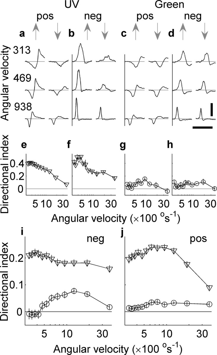
Responses of an L-neuron to colored bars moving vertically upward or downward. a, UV, positive contrast. b, UV, negative contrast. Responses to upward bars (below the upward arrows) are larger than those to downward bars (below the downward arrows). The different rows show the responses for different angular velocities as indicated by the numbers to the left side of the figure in units of degrees per second. Each trace is the average of two trials. c and d show the corresponding responses to green bars. In this case, there is little difference in the response. Calibration: vertical, 5 mV; horizontal, 250 ms. e–h indicate the directional indices obtained from the responses shown in the column above them (a–d). Only a quarter of the angular velocities used to determine the directional indices in e–h are shown in a–d. Pooled directional indices of 48 L-neurons are shown for negative contrast bars (i) and positive contrast bars (j). Triangles indicate that UV bars were used, and circles indicate green bars were the stimuli. Error bars indicate SEM. Differences between positive and negative contrasts indicate nonlinearities in the response.

To quantify the directionality of these responses, the DI was calculated from the peak-to-peak intracellular response of the neuron in the 500 ms after upward and downward moving bars (see Materials and Methods). The directional indices for the responses, shown in Figure 1, a–d, are shown in e–h, respectively. The maximum DI in the case of UV bars was 0.5 for a negative contrast bar moving at 536° s⁻¹, which means the response to an upward moving bar is three times the magnitude of the response to a downward moving bar. The maximum directionality of the response to a green bar for this cell was 0.16 and occurred for a positive contrast bar moved at 938° s⁻¹, indicating that the response to an upward moving bar was 40% greater than the reverse.

The pooled data from 48 cells are presented in Figure 1i, which shows the DIs for UV (triangles) and green (circles) negative contrast bars, and in Figure 1j, which shows the DIs for UV and green positive contrast bars. Negative contrast green bars produced DIs that were not significantly different from zero for speeds between 312.5 and 535.7° s⁻¹ (p > 0.2; n = 44; unpaired t test), whereas for positive contrast bars the range in which no difference was found was 312.5–468.75° s⁻¹ (p > 0.13; n = 44; unpaired t test). UV positive or negative contrast bars were significantly different from zero in all cases (negative contrast bars, values of p < 10⁻¹⁵, n = 47, unpaired t test; and positive contrast bars, values of p < 10⁻¹³, n = 48, unpaired t test).

On average, negative contrast bars produce stronger directional responses at very high velocities than positive contrast bars. The average optimal velocity across the cell population for negative contrast bars was 742° s⁻¹ (SD, 727 °s⁻¹; n = 48), which was slightly higher and more variable than for positive contrast bars: 727° s⁻¹ (SD, 335° s⁻¹; n = 48).

Responses to gratings

To test the robustness of the directional response, we tested contrast gratings of different wavelengths and different speeds. These also elicited directional responses, and again this was highly dependent on the wavelength of the light used: green gratings produced almost no directionality. The directionality, like that in the case of bars, is encoded in the magnitude of the response modulation, and not in its mean. Responses to UV gratings moved at 1250° s⁻¹ are shown in Figure 2, a–c, with the direction of the grating movement indicated by the arrows. The three different rows represent different spatial wavelengths ranging from 24 to 72° (indicated in each row). Directional indices were determined from the root mean squared responses (see Materials and Methods). This cell demonstrates robustness in its directional response to changes in the spatial wavelength of the UV grating being shown (see DI indicated). When the same gratings shown at the same speed are changed from UV to green, the directionality effectively disappears (shown in Fig. 2d–f).

Figure 2.

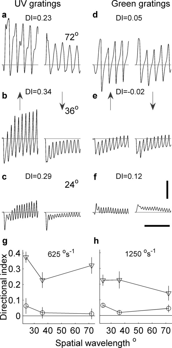
Responses of an L-neuron to colored gratings moving vertically up and down (directions indicated by arrows). a–c show the responses to UV gratings with the same velocity of 1250° s⁻¹ but three different spatial wavelengths (a, 72°; b, 36°; c, 24°). The directionality of each pair of responses is indicated by the DIs. d–f show the responses to the same patterns as those in a–d, but in this case the patterns were green. Calibration: vertical, 5 mV; horizontal, 200 ms. Note that a negative DI indicates there is a greater root mean squared response to the downward moving grating than the upward one. g, The pooled directional indices are shown for gratings colored UV (triangles) and green (circles) moved at 625° s⁻¹. A total of n = 24 cells were shown both UV and green. h, Responses for the same cells as in g but for a faster grating speed of 1250° s⁻¹. In the cases in which UV gratings were used, all the DIs were significantly different from zero (speed, 625° s⁻¹: λ = 24°, p < 4 × 10⁻⁵, n = 7, unpaired t test; λ = 36°, p < 0.016, n = 7, Wilcoxon's rank test, and λ = 36°, p < 0.016, n = 7, Wilcoxon's rank test; speed, 1250° s⁻¹: λ = 24°, n = 18, p < 4 × 10⁻⁹, unpaired t test; λ = 36°, p < 2 × 10⁻⁶, n = 18, unpaired t test, and λ = 72°, p < 6 × 10⁻⁵, n = 18, unpaired t test). The DI values for green gratings were only significantly different from zero for λ = 24° and speed of 625° s⁻¹ (p < 3 × 10⁻⁴; n = 6; Wilcoxon's rank test); the other DI values were not significantly different from zero (speed, 1250 °s⁻¹: λ = 24°, p > 0.25, n = 18, unpaired t test; λ = 36°, p > 0.2, n = 18, unpaired t test; λ = 72°, speed, 1250° s⁻¹, p > 0.2, n = 18, Wilcoxon's rank test; and speed, 625° s⁻¹: λ = 36°, p > 0.6, n = 6, unpaired t test, and λ = 72°, p > 0.55, n = 6, Wilcoxon's rank test).

Figure 2, g and h, shows the pooled directional indices from 24 cells using UV gratings (triangles) and green gratings (circles), for a range of spatial wavelengths and at two different speeds: 625° s⁻¹ (Fig. 2g) and 1250° s⁻¹ (Fig. 2h). In only one case were the green DIs significantly different from zero, that is, for gratings with a wavelength of 24° and moving at 625° s⁻¹ (Fig. 2). However, this was on average small (DI = 0.07), indicating that the RMS response was on average ∼15% greater for an upward moving green grating compared with a downward moving green grating. In all other cases, the DI distribution was not significantly different from zero. In the cases in which UV gratings were moved at a speed of 625° s⁻¹, all the DIs were significantly different from zero, as was the case when the grating was moved at 1250° s⁻¹ (Fig. 2).

Although we could not display oblique angles because of the limited resolution of the display, we tested whether horizontally moving gratings produced directionally selective responses. The mean DI for 21 cells shown vertically oriented gratings moved horizontally (wavelength, 42°; speed, 1250° s⁻¹) was −0.08 (SD, 0.13), whereas the DI for the same cells measured using horizontally oriented gratings moved vertically (wavelength, 36°; speed, 1250° s⁻¹) was 0.19 (SD, 0.15). These results indicate that the preferred stimulus orientation of these cells is horizontal.

STRFs

The results above for the first time show that neurons receiving visual input from the median ocellus alone have directional selective response properties. To further investigate the color-dependent directional effects in L-neuron responses, we determined their UV and green linear STRFs separately, using reverse-correlation analysis. This process is represented in Figure 3, where six example frames from the UV stimulus are depicted in Figure 3a and the intracellular response to a similar but longer UV stimulus sequence is shown in Figure 3b by the gray line. The black line in Figure 3b indicates the linear prediction from the measured STRFs (shown in Fig. 3c). On average, responses to white noise stimuli were well described by the STRFs with UV STRFs producing MSPEs of 18.3% (SD, 17.2%; n = 54) and green STRFs producing MSPEs of 27.6% (SD, 17.4%; n = 51). The difference in errors was statistically significant (paired t test, p < 0.007), which is consistent with the significantly higher signal-to-noise ratio in the response to a UV stimulus (mean, 34.5; SD, 28.8; n = 59) compared with the green stimulus (mean, 15.0; SD, 13.0; n = 58; p < 10⁻⁶, Wilcoxon's rank test). An estimate of the relative power in the unfitted nonlinear (Wiener) terms compared with the detrended signal power can be estimated by subtracting the power in the noise from the MSPE defined in Equation 2. Using this method, the unfitted components accounted for 25% in the case of UV stimuli and 21% in the case of green stimuli. Thus, cells responded more linearly and with greater noise to green stimuli than to UV stimuli.

Figure 3.

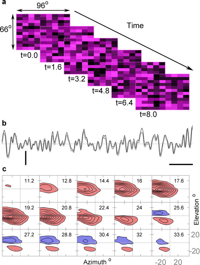
The reverse-correlation method for mapping spatiotemporal receptive fields. a, A representation of six frames of the random UV stimulus. Each frame is separated by 1.6 ms. b, The intracellular response of an L-neuron to random stimulation by UV light (thick gray line). The thinner dark line indicates the response predicted by the derived UV spatiotemporal receptive field (UV STRF) shown in c. The mean squared prediction error for this cell is 10.3% and the separability index is α = 0.13. Only a small portion of the 40 s stimulus is shown. Calibration: vertical, 2 mV; horizontal, 100 ms. c, The STRF is shown from time t = 11.2 ms to t = 33.6 ms. The time of each two-dimensional profile is indicated in milliseconds, in the top right of each frame. The blue shaded areas represent depolarizations to light increments and the red shaded areas hyperpolarizations to light increments. Contours are at 10% increments of the maximum absolute value of the STRF, which is 0.24 mV/(C ms).

An example of an estimated STRF for UV is shown in Figure 3c, showing the two-dimensional spatial structure in frames from t = 11.2 to 33.6 ms, in time increments of 1.6 ms. There is no noticeable effect for the first 9.6 ms (data not shown), likely to be attributable to the combination of the latency of phototransduction in the photoreceptors and the synaptic delay from photoreceptors to L-neuron. Thereafter, a pronounced receptive field emerges, reaching its maximum at t = 19.2 ms. In the following frames, the response in the upper one-half of the receptive field decays and eventually reverses polarity, becoming positive (indicated by blue shading). During this process, the negative lobe (indicated by red shading) appears to be changing position in a downward direction while it is decaying; to a lesser extent, the positive lobe moves downward, albeit with a delay.

STRFs obtained with both UV and green stimuli, which were measured separately for the same cell, are shown in Figure 4, a and g, respectively. In this case, two-dimensional angular profiles are shown for four different delays. Although in the first frame the green and UV STRFs appear to be similarly located, as time progresses there is a downward drift in the UV receptive field but not in the green field. It turns out that we can account for this drift by decomposing the full STRF into a space–time separable component (shown in Fig. 4c for UV and Fig. 4i for green) and a residual (shown in Fig. 4e for UV and Fig. 4k for green) (see Materials and Methods). In the case of the green STRF, the residual component is negligible (Fig. 4k), indicating that the green receptive field is mostly separable into spatial and temporal components. However, the UV STRF has a significant inseparable component (Fig. 4e). The two lobes of this component define the preferred stimulus orientation (see Materials and Methods) that in this case is −30° (±15°).

Does the difference in the separability of the UV and green STRFs account for the differences in directionality and what are the nonlinear and linear components of directional selectivity? By comparing the STRF predictions (linear predictions) of the response with the measured responses, we can examine these questions. Examples are shown for the predicted (black line) and measured (gray line) responses to UV and green positive contrast bars in Figure 4, b and h, respectively. In the case of UV bars, there is a small discrepancy between the measured response and response predicted by the full UV STRF. Importantly, the predicted response produces the same directional sensitivity as the measured response. In the case of green bars, the measured response is poorly predicted by the green STRF, indicating significant nonlinearities in the response. However, the green STRF does predict responses that show the same insensitivity to the direction of the bar. So in both UV and green cases the directionality or lack of it is reproduced by the predicted response from the full STRFs.

Figure 4 demonstrates that the directionality in the UV response is produced by the inseparable residual of the UV STRF. The response predicted by its separable component, shown in Figure 4d, shows little directionality, whereas the response predicted by the residual UV STRF (Fig. 4f) produces waveforms with opposite polarities, albeit with similar amplitudes. The residual waveform for an upward moving bar adds to the response predicted by the separable component of the STRF, whereas for the downward moving bar, the residual waveform subtracts from the separable response. Note that the response predicted by the residual component of the green STRF (Fig. 4l) is negligible.

The pooled linear predictions of the DIs for 47 L-neurons, based on the estimated STRFs, are shown in Figure 5, a and b, for UV (circles) and green (triangles) bars. These are plotted alongside the measured DIs for the same cells. Figure 5a shows the measured and predicted DIs for negative contrast bars, whereas Figure 5b similarly shows the DI values for positive contrast bars. The correlation between the measured and predicted DIs was strongest for positive contrast UV bars (mean r² = 0.49; SD, 0.35; n = 44), which were significantly larger than those for negative contrast bars (mean r² = 0.33; SD, 0.30; n = 44; p < 0.016, Wilcoxon's rank test).

Figure 5.

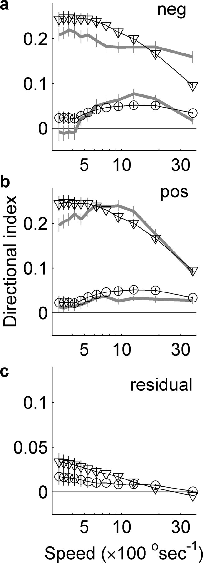
The STRF predicted (dark lines) and measured (thick gray lines) DIs for negative (a) and positive (b) contrast bars pooled for 47 L-neurons. DIs were predicted from the full UV (triangles) or green (circles) STRF. c shows the directional index of the separable components of the STRFs as shown in Figures 4, e and k, with triangles and squares as in a and b. STRFs were better predictors for the DIs measured with UV positive contrast bars, indicating that directional nonlinear mechanisms respond mainly to negative contrast UV bars. These nonlinear mechanisms enhance directionality at high velocities and inhibit it at lower velocities.

At the optimal speed, predicted DIs were 93.7% (SD, 42%; n = 44) of the measured value for negative contrast bars and 84% (SD, 25%; n = 44) of the value for positive contrast bars. However, there were no significant differences between the r² values for negative contrast UV bars, positive contrast green bars (mean r² = 0.28; SD, 0.25; n = 43), or negative contrast green bars (mean r² = 0.23; SD, 0.22; n = 42) (p > 0.5, Kruskal–Wallis one-way ANOVA). Thus, STRFs were best at predicting the DIs for positive contrast UV bars at the optimal angular velocity.

The r² values for gratings (UV, mean r² = 0.62; SD, 0.39; green, mean r² = 0.63; SD, 0.32) suggest that STRFs are better at predicting the directionality of the responses to gratings than to bars, except in the case of positive contrast UV bars. At the optimal spatial frequency, we found that the STRF prediction of the DI was better at 625° s⁻¹, where it was 89% of the measured value (SD, 25%; n = 9) compared with the 59% (SD, 54%; n = 8) at the grating speed of 1250° s⁻¹. As with the results from the bars, this suggests that nonlinearities play a significant role in modulating the response at high velocities.

The largest difference between predicted and measured directional indices occurs at high velocities for UV bars indicating nonlinear mechanisms act to enhance the bandwidth of directional selectivity to negative contrast bars over positive contrast bars. By removing the inseparable component of the STRFs and predicting the DIs (Fig. 5c), the predicted mean directionality becomes 8.7% of that predicted by the full STRF for UV and 38.3% for green. From these results, we may conclude that the space–time inseparability of the STRFs is primarily responsible for their directionality in UV light, but a large proportion of directionality seen in green light is the result of directional nonlinearities.

Figure 6 summarizes the results of all cells shown for either gratings or bars. Figure 6a shows a scatter plot of the directional index in UV versus green for both bars and gratings. Mean values for UV gratings were 0.33 (SD, 0.10; n = 24) and for UV bars was 0.29 (SD, 0.09; n = 84). The mean DI values for green gratings was 0.10 (SD, 0.10; n = 24) and for green bars was 0.12 (SD, 0.06; n = 84). In the case of either bars or gratings, the UV DIs were significantly larger than those for the equivalent green pattern (bars, p < 10⁻¹⁰, Wilcoxon's rank test; and gratings, p < 10⁻⁶, paired t test).

Figure 6.

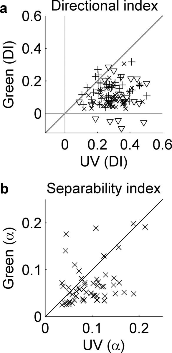
Scatter plot of maximum DIs for positive contrast bars (45° crosses), negative contrast bars (90° crosses), and gratings (triangles) with UV DIs along the ordinate and green DIs along the abscissa (a). b, Scatter plot of the green versus UV separability index α for all cells studied in the paper. An α of zero indicates that the STRF can be perfectly reconstructed by its spatial and temporal components.

Figure 6b shows the separability index (α), which indicates the power in the separable residual as a percentage of the STRF power, plotting UV against green for the same cell. An equal residual in each would put the cell on the line of equality and indicate that an equal level of separability exists in both UV and green STRFs. Clearly, the STRFs show greater inseparability in UV light (mean, 0.10; SD, 0.05; n = 57) than in green (0.07; SD, 0.04; n = 57), and this is statistically significant (paired t test, p < 0.0015). The difference in separability between UV and green receptive fields was unlikely to be attributable to the fact that responses to green contrasts were smaller than they were to UV because there was very little correlation between the RMS response and α (UV, r² = 0.006, n = 57; and green, r² = 0.004, n = 57).

Contribution of the compound eyes

Given the small latencies of the L-neuron responses, it would appear unlikely that compound eyes contribute to the directionality through synaptic connections. However, there is growing evidence that fast electrical connections couple ocellar and visual interneurons (Parsons et al., 2006; Haag et al., 2007). These fast connections could theoretically transfer directional selectivity computed in compound eye interneurons to the median ocellar L-neurons. We therefore blocked the compound eyes with paint to assess their contribution, if any, to the directional responses of L-neurons. We recorded the directionality to negative contrast bars. The mean DI was 0.33 (SD, 0.09; n = 10), which was not significantly different from the cases in which the compound eye had not been covered (p < 0.05). We also measured the UV receptive fields for these cells. They demonstrated the same drift in space with time as occurred in previous STRFs. The mean SI was 0.18 (SD, 0.08; n = 10), which was also not significantly different from previous results in which the compound eye had not been covered (p < 5 × 10⁻⁴). Thus, the directionality seen in L-neurons does not originate from the compound eye.

Discussion

We have shown that the L-neurons of the median ocellus of the dragonfly respond in a directionally selective manner to UV colored vertically moving bars and gratings. Overall, nonlinearities appear to play only a minor role because the directionality in the responses is predicted by the linear UV STRFs. Nonlinear responses do, however, act to enhance directionality at high velocities (3750° s⁻¹) and inhibit them at lower velocities (<1000° s⁻¹) for negative UV contrasts. The magnitude of the directionality found here in ocellar L-neurons (UV gratings: mean DI, 0.33; SD, 0.10; UV bars: mean DI, 0.30; SD, 0.07) is remarkably similar to values obtained from intracellular recordings of simple cells of the mammalian visual cortex, where it has been estimated to be 0.28 (SD, 0.21) (Carandini and Ferster, 2000). In that case, grating stimuli were used. Previous studies of insects other than the dragonfly have inferred from anatomical and optical evidence that individually ocelli are not capable of computing directional information (Parry, 1947; Wilson, 1978; Wehner, 1987; Schuppe and Hengstenberg, 1993; Mizunami, 1994) but instead have ocelli that act together, each as a single sensor (Stange, 1981; Wehner, 1987; Schuppe and Hengstenberg, 1993; Parsons et al., 2006). However, these studies did not explicitly test for directional selectivity. Thus, it remains an open question whether the L-neurons in the ocelli of other insect species are directionally selective.

We found that dragonfly median ocellar L-neurons encode directionality in the response modulation and not the response mean. This phenomenon has been seen widely in the retinal cells of other invertebrates and vertebrates (Clifford and Ibbotson, 2003) and higher visual centers such as the mammalian visual cortex (DeAngelis et al., 1993; Jagadeesh et al., 1993; Clifford and Ibbotson, 2003). In simple cells of the mammalian visual cortex, this type of directionality been shown to arise from spatiotemporal inseparabilities in the STRFs of those cells, or in other words, changes in the temporal response shape with changes in spatial location (DeAngelis et al., 1993; Jagadeesh et al., 1993). These linear filters have previously been proposed to form the early stages of energy motion detection models (Adelson and Bergen, 1985; van Santen and Sperling, 1985; Watson and Ahmuda, 1985). We observed the same inseparabilities in the UV STRFs of L-neurons. This type of directional computation is distinct from that seen in fully opponent directionally selective cells, like lobula plate tangential cells in flies (Hausen, 1982a,b; Single et al., 1997; Borst and Haag, 2002; Egelhaaf et al., 2002) or complex cells in the mammalian visual cortex (Emerson et al., 1992) that encode directionality in the mean of the response.

Another feature that distinguishes the directional responses seen here from those previously recorded in insects is the spatial scale on which the computation takes place. In L-neurons, the directionality is calculated over several tens of degrees, whereas directionality in interneurons fed by the compound eye is of the order of a few degrees (McCann, 1973; Franceschini et al., 1989). L-neuron directionality is therefore predicted to be mostly dependent on the spatial characteristics of the moving stimulus, a prediction that is confirmed by our results (Fig. 2).

Theoretical considerations suggest that, in order for visual neurons to produce useable, time-averaged directional signals, they must perform a nonlinear computation (Hassenstein and Reichardt, 1956; Poggio and Reichardt, 1973). In the case of the simple cells of the mammalian cortex, for example, the nonlinear relationship between synaptic input and spike generation assists in performing this task (Carandini and Ferster, 2000). In the case of the dragonfly median ocellus, it is possible that nonlinear processing occurs at the next synaptic level (the L2 to L3 synapse), because studies on cockroach ocelli have established that these synapses are rectifying (Mizunami, 1996). However, it is more difficult to see how the ocellus could produce an opponent mechanism that would inhibit responses to downward movements, because all ocellar neurons have the same preference for upward movements.

The mechanisms underlying the spatiotemporal inseparability seen in the median ocellar UV STRFs involve asymmetries between the upper and lower halves of the receptive field. There are several candidate mechanisms capable of producing these asymmetries including inhibitory synapses between L-neurons, influences of small neurons, or feedback from photoreceptors. Dendritic delays may also play a role as three-dimensional reconstructions suggest that, for some cells at least, there is a difference in the pattern of dendritic branching between the upper and lower parts of the receptive field (Berry et al., 2006). Additional studies are required to probe the relative contributions of these cellular processes to the motion sensitivity.

Our results show that, during the day, the directionality of L-neurons is broadly tuned to fast (100–3750° s⁻¹) movements and mostly dependent on UV light. This suggests that the role for the median ocellus under light intensities equivalent to daylight conditions is to produce UV self-movement information, whereas motion detectors fed from the compound eye are tuned to green patterns (Olberg, 1981a,b; Horridge et al., 1990). Directional responses at the high speeds used here have been observed in insect neurons that receive compound eye input (Olberg, 1981a; Ibbotson, 1991; O'Carroll et al., 1996; Lewen et al., 2001; David et al., 2004). Therefore, it would appear that the main advantage of the median ocellus, over the compound eye, lies in the speed with which it can transmit signals down the ventral nerve chord to motor centers rather than its ability to detect fast motion; ocellar signals have been shown to be some 10–20 ms faster than signals transmitted from the compound eye (Olberg, 1981b). Behavioral evidence from locusts also indicates that visually evoked head movements with short latencies (<100 ms) are dependent on ocelli (Taylor, 1981).

Recently, receptive field structures in mammals have been shown to be dependent on image statistics (David et al., 2004) and this adaptation has been shown to increase the information coding capacity of the neurons (Sharpee et al., 2006). In addition to this, indirect evidence suggests that the receptive field structure of visually driven cells in monkeys and cats is also dependent on the contrast of the stimulus (Priebe et al., 2006; Crowder et al., 2007). Our results add to these studies by showing that receptive field structures can also alter with the changing spectral wavelength of the stimulus even if the stimulus statistics and contrast are identical. Moreover, we have shown that the function of this adaptation in the dragonfly median ocellus is to allow computation of directional information about wide-field moving edges. Given that the median ocellus points frontally, it would appear this information is optimized for detecting changes in pitch (Neumann and Bülthoff, 2002; Schenato et al., 2004).

Although it is clear from our results that the L-neurons of the median ocellus are directional under light-adapted conditions, it is difficult to extrapolate their functionality at low light levels. It has been well established from intracellular recordings of L-neurons (Mobbs et al., 1981) and behavioral experiments (Stange, 1981) that the ocellar system undergoes a reverse Purkinje shift becoming more green-sensitive at low light levels. Given this, it would be tempting to conclude that, at low light levels, these eyes act as single sensors. However, it is possible that the green-sensitive channels show the same directional selectivity at low light levels as UV channels show under the photopic conditions. Only additional testing at low light levels will settle this question.

The results reported here are consistent with and extend the original work done by Zenkin and Pigarev (1971). However, it is impossible to make a quantitative comparison between our study and theirs because they did not include any quantitative data on the directional responses they measured. Our results suggest a reason why their stimulus successfully elicited directional responses from the ocelli. Somewhat unusually for the time, they performed the experiments outside in the sun where there is an abundance of UV light, and, as we have demonstrated, this is an optimal condition for producing directional responses in the dragonfly median ocellus.

References

- Adelson EH, Bergen JR. Spatiotemporal energy models for the perception of motion. J Opt Soc Am A. 1985;2:284–299. doi: 10.1364/josaa.2.000284. [DOI] [PubMed] [Google Scholar]
- Berry R, Stange G, Olberg R, van Kleef J. The mapping of visual space by identified large second-order neurons in the dragonfly median ocellus. J Comp Physiol A Neuroethol Sens Neural Behav Physiol. 2006;192:1105–1123. doi: 10.1007/s00359-006-0142-5. [DOI] [PubMed] [Google Scholar]
- Berry R, van Kleef J, Stange G. The mapping of visual space by dragonfly lateral ocelli. J Comp Physiol A Neuroethol Sens Neural Behav Physiol. 2007a;193:495–513. doi: 10.1007/s00359-006-0204-8. [DOI] [PubMed] [Google Scholar]
- Berry RP, Stange G, Warrant EJ. Form vision in the insect dorsal ocelli: an anatomical and optical analysis of the dragonfly median ocellus. Vision Res. 2007b;47:1394–1409. doi: 10.1016/j.visres.2007.01.019. [DOI] [PubMed] [Google Scholar]
- Borst A, Haag J. Neural networks in the cockpit of the fly. J Comp Physiol. 2002;188:419–437. doi: 10.1007/s00359-002-0316-8. [DOI] [PubMed] [Google Scholar]
- Carandini M, Ferster D. Membrane potential and firing rate in cat visual cortex. J Neurosci. 2000;20:470–484. doi: 10.1523/JNEUROSCI.20-01-00470.2000. [DOI] [PMC free article] [PubMed] [Google Scholar]
- Chappell RL, Dowling JE. Neural organization of the median ocellus of the dragonfly. I. Intracellular electrical activity. J Gen Physiol. 1972;60:121–147. doi: 10.1085/jgp.60.2.121. [DOI] [PMC free article] [PubMed] [Google Scholar]
- Clifford CWG, Ibbotson MR. Fundamental mechanisms of visual motion detection: models, cells and functions. Prog Neurobiol. 2003;68:409–437. doi: 10.1016/s0301-0082(02)00154-5. [DOI] [PubMed] [Google Scholar]
- Crowder NA, van Kleef J, Dreher B, Ibbotson MR. Complex cells increase their phase-sensitivity at low contrasts and following adaptation. J Neurophysiol. 2007;98:1155–1166. doi: 10.1152/jn.00433.2007. [DOI] [PubMed] [Google Scholar]
- David SV, Vinje WE, Gallant JL. Natural stimulus statistics alter the receptive field structure of V1 neurons. J Neurosci. 2004;24:6991–7006. doi: 10.1523/JNEUROSCI.1422-04.2004. [DOI] [PMC free article] [PubMed] [Google Scholar]
- DeAngelis GC, Ohzawa I, Freeman RD. Spatiotemporal organization of simple-cell receptive fields in the cat's striate cortex. I. General characteristics and postnatal development. J Neurophysiol. 1993;69:1091–1117. doi: 10.1152/jn.1993.69.4.1091. [DOI] [PubMed] [Google Scholar]
- Depireux DA, Simon JZ, Klein DJ, Shamma SA. Spectro-temporal response field characterization with dynamic ripples in ferret primary auditory cortex. J Neurophysiol. 2001;85:1220–1234. doi: 10.1152/jn.2001.85.3.1220. [DOI] [PubMed] [Google Scholar]
- Dowling JE, Chappell RL. Neural organization of the median ocellus of the dragonfly. II. Synaptic structure. J Gen Physiol. 1972;60:148–165. doi: 10.1085/jgp.60.2.148. [DOI] [PMC free article] [PubMed] [Google Scholar]
- Egelhaaf M, Kern R, Krapp HG, Kretzberg J, Kurtz R, Warzecha A-K. Neural encoding of behaviourally relevant visual-motion information in the fly. Trends Neurosci. 2002;25:96–102. doi: 10.1016/s0166-2236(02)02063-5. [DOI] [PubMed] [Google Scholar]
- Emerson RC, Bergen JR, Adelson EH. Directionally selective complex cells and the computation of motion energy in cat visual cortex. Vision Res. 1992;32:203–218. doi: 10.1016/0042-6989(92)90130-b. [DOI] [PubMed] [Google Scholar]
- Franceschini N, Riehle A, Le Nestour A. Directionally sensitive motion detection by insect neurons. In: Stavenga DG, Hardie RC, editors. Facets of vision. Berlin: Springer; 1989. pp. 360–389. [Google Scholar]
- Haag J, Wertz A, Borst A. Integration of lobula plate output signals by DNOVS1, an identified premotor descending neuron. J Neurosci. 2007;27:1992–2000. doi: 10.1523/JNEUROSCI.4393-06.2007. [DOI] [PMC free article] [PubMed] [Google Scholar]
- Hassenstein B, Reichardt W. Systemtheoretische Analyse der Zeit-, reihenfolgen- und Vorzeichenauswertung bei der Bewegungsperzeption des Rüsselkäfers Chlorophanus. Z Naturforsch. 1956;11b:513–524. [Google Scholar]
- Hausen K. Motion sensitive interneurons in the optomotor system of the fly. I. The horizontal cells: structure and signals. Biol Cybernet. 1982a;45:143–156. [Google Scholar]
- Hausen K. Motion sensitive interneurons in the optomotor system of the fly. II. The horizontal cells: receptive field organization and response characteristics. Biol Cybernet. 1982b;46:67–79. [Google Scholar]
- Horridge GA, Wang X, Zhang SW. Colour inputs to motion and object vision in an insect. Philos Trans R Soc Lond B Biol Sci. 1990;329:257–263. [Google Scholar]
- Ibbotson M. A motion-sensitive visual descending neurone in Apis mellifera monitoring translatory flow-fields in the horizontal plane. J Exp Biol. 1991;157:537–577. [Google Scholar]
- Jagadeesh B, Wheat HS, Ferster D. Linearity of summation of synaptic potentials underlying directional selectivity in simple cells of the cat visual cortex. Science. 1993;262:1901–1904. doi: 10.1126/science.8266083. [DOI] [PubMed] [Google Scholar]
- James AC. The pattern-pulse multifocal visual evoked potential. Invest Ophth Vis Sci. 2003;44:879–890. doi: 10.1167/iovs.02-0608. [DOI] [PubMed] [Google Scholar]
- Juusola M, Niven JE, French AS. Shaker K+ channels contribute early nonlinear amplification to the light response in Drosophila receptors. J Neurophysiol. 2003;90:2014–2021. doi: 10.1152/jn.00395.2003. [DOI] [PubMed] [Google Scholar]
- Lewen GD, Bialek W, de Ruyter van Steveninck RR. Neural coding of naturalistic motion stimuli. Network. 2001;12:317–329. [PubMed] [Google Scholar]
- Livingston MS, Conway BR. Substructure of directionally selective receptive fields in macaque V1. J Neurophysiol. 2003;89:2743–2759. doi: 10.1152/jn.00822.2002. [DOI] [PMC free article] [PubMed] [Google Scholar]
- McCann GD. The fundamental mechanism of motion detection in the insect visual system. Kybernetik. 1973;12:64–73. doi: 10.1007/BF00272462. [DOI] [PubMed] [Google Scholar]
- Mittelstaedt H. Physiologie des Gleichgewichtssinnes bei fliegenden Libellen. Z Vergl Physiol. 1950;3a:421–463. [PubMed] [Google Scholar]
- Mizunami M. Functional diversity of neural organization in insect ocellar systems. Vision Res. 1994;35:443–452. doi: 10.1016/0042-6989(94)00192-o. [DOI] [PubMed] [Google Scholar]
- Mizunami M. Gain control of synaptic transfer from second- to third-order neurons of cockroach ocelli. J Gen Physiol. 1996;107:121–131. doi: 10.1085/jgp.107.1.121. [DOI] [PMC free article] [PubMed] [Google Scholar]
- Mobbs PG, Guy RG, Goodman LJ, Chappell RL. Relative spectral sensitivity and reverse Purkinje shift in identified L-neurons of the ocellar retina. J Comp Physiol A Neuroethol Sens Neural Behav Physiol. 1981;144:91–97. [Google Scholar]
- Neumann TR, Bülthoff HH. Behavior-oriented vision for biomimetic flight control. EPSRC/BBSRC International Workshop on Biologically Inspired Robotics: The Legacy of W. Grey Walter; 8; Bristol, UK. 2002. Paper presented at. [Google Scholar]
- O'Carroll DC, Bidwell NJ, Laughlin SB, Warrant EJ. Insect motion detectors matched to visual ecology. Nature. 1996;382:63–66. doi: 10.1038/382063a0. [DOI] [PubMed] [Google Scholar]
- Olberg RM. Object and self-movement detectors in the ventral nerve cord of the dragonfly. J Comp Physiol A Neuroethol Sens Neural Behav Physiol. 1981a;141:327–334. [Google Scholar]
- Olberg RM. Parallel encoding of direction of wind, head, abdomen and visual pattern movement by single interneurons in the dragonfly. J Comp Physiol A Neuroethol Sens Neural Behav Physiol. 1981b;142:27–41. [Google Scholar]
- Parry DA. The function of the insect ocellus. J Exp Biol. 1947;24:211–219. doi: 10.1242/jeb.24.3-4.211. [DOI] [PubMed] [Google Scholar]
- Parsons MM, Krapp HG, Laughlin SB. A motion-sensitive neurone responds to signals from the two visual systems of the blowfly, the compound eyes and ocelli. J Exp Biol. 2006;209:4464–4474. doi: 10.1242/jeb.02560. [DOI] [PubMed] [Google Scholar]
- Poggio T, Reichardt W. Considerations on models of movement detection. Kybernetik. 1973;13:223–227. doi: 10.1007/BF00274887. [DOI] [PubMed] [Google Scholar]
- Priebe NJ, Lisberger SG, Movshon JA. Tuning for spatiotemporal frequency and speed in directionally selective neurons of macaque striate cortex. J Neurosci. 2006;26:2941–2950. doi: 10.1523/JNEUROSCI.3936-05.2006. [DOI] [PMC free article] [PubMed] [Google Scholar]
- Schenato L, Wu WC, Sastry S. Attitude control for a micromechanical flying insect via sensor output feedback. IEEE Trans Rob Autom. 2004;20:93–106. [Google Scholar]
- Schuppe H, Hengstenberg R. Optical properties of the ocelli of Calliphora erythrocephala and their role in the dorsal light response. J Comp Physiol A Neuroethol Sens Neural Behav Physiol. 1993;173:143–149. [Google Scholar]
- Sharpee TO, Sugihara H, Rebrik S, Kurgansky A, Stryker MP, Miller KD. Adaptive filtering enhances information transmission in visual cortex. Nature. 2006;439:936–942. doi: 10.1038/nature04519. [DOI] [PMC free article] [PubMed] [Google Scholar]
- Simmons PJ. The operation of connections between photoreceptors and large 2nd order neurones in dragonfly ocelli. J Comp Physiol A Neuroethol Sens Neural Behav Physiol. 1982;149:389–398. [Google Scholar]
- Single S, Haag J, Borst A. Dendritic computation of direction selectivity and gain control in visual interneurons. J Neurosci. 1997;17:6023–6030. doi: 10.1523/JNEUROSCI.17-16-06023.1997. [DOI] [PMC free article] [PubMed] [Google Scholar]
- Stange G. The ocellar component of flight equilibrium control in dragonflies. J Comp Physiol A Neuroethol Sens Neural Behav Physiol. 1981;141:335–347. [Google Scholar]
- Stange G, Howard J. An ocellar dorsal light response in a dragonfly. J Exp Biol. 1979;83:351–355. [Google Scholar]
- Stange G, Stowe S, Chahl JS, Massaro A. Anisotropic imaging in the dragonfly median ocellus: a matched filter for horizon detection. J Comp Physiol A Neuroethol Sens Neural Behav Physiol. 2002;188:455–467. doi: 10.1007/s00359-002-0317-7. [DOI] [PubMed] [Google Scholar]
- Taylor CP. Contribution of compound eyes and ocelli to steering of locusts in flight. I. Behavioural analysis. J Exp Biol. 1981;93:1–18. [Google Scholar]
- van Kleef J, James AC, Stange G. A spatiotemporal white noise analysis of photoreceptor responses to UV and green light in the dragonfly median ocellus. J Gen Physiol. 2005;126:481–497. doi: 10.1085/jgp.200509319. [DOI] [PMC free article] [PubMed] [Google Scholar]
- van Santen JPH, Sperling G. Elaborated Reichardt detectors. J Opt Soc Am A. 1985;2:300–321. doi: 10.1364/josaa.2.000300. [DOI] [PubMed] [Google Scholar]
- Watson AB, Ahmuda AJ. Model of human visual motion sensing. J Opt Soc Am A. 1985;2:322–342. doi: 10.1364/josaa.2.000322. [DOI] [PubMed] [Google Scholar]
- Wehner R. Matched-filters—neural models of the external world. J Comp Physiol A Neuroethol Sens Neural Behav Physiol. 1987;161:511–531. [Google Scholar]
- Wilson M. The functional organisation of locust ocelli. J Comp Physiol A Neuroethol Sens Neural Behav Physiol. 1978;124:297–316. [Google Scholar]
- Zenkin GM, Pigarev IN. Optically determined activity in the cervical nerve chain of the dragonfly. Biofizika. 1971;16:299–306. [PubMed] [Google Scholar]