Preparing to Move Increases the Sensitivity of Superior Colliculus Neurons

Abstract

How the brain selects goals for movements remains unknown. The system designed to move the eyes rapidly, the saccadic system, may play a role. Here we ask how sensory signals within a saccade area are influenced by selecting and preparing a saccade. Trained monkeys made or withheld saccades, based on a color cue, to targets varying in luminance contrast. We measured the initial visual activity of superior colliculus (SC) neurons in response to the appearance of these targets. We determined neuronal contrast responses in three task conditions: when two luminance gratings appeared one in the response field (RF) and one in the mirror-opposite location and a cue to select the stimulus in the RF occurred; when the gratings appeared and a cue to select the stimulus out of the RF occurred; and third, when the gratings appeared but monkeys remained fixating on the central spot. SC neurons had increases in visual responses when contrast increased. Receiver operating characteristic analysis revealed an increased ability of neurons to detect the grating on trials with higher contrast targets and also on trials with a cue to make a saccade compared with trials with a cue to remain fixating. Using two measures of neuronal sensitivity, those SC neurons considered part of the motor circuitry increased their sensitivity to contrast with a cue to make a saccade. The results indicate that movement commands influence sensory responses in SC in much the same way that commands to shift attention influence sensory responses in extrastriate cortex.

Introduction

Spatial attention enhances sensory signals to facilitate processing (Maunsell, 1995; Egeth and Yantis, 1997; Colby and Goldberg, 1999; Ungerleider and Kastner, 2000; Reynolds and Chelazzi, 2004; Wolfe and Horowitz, 2004). Evidence from the motor system designed to move the eyes rapidly, the saccadic system, indicates that brain regions critical for the generation of saccades play an active role in shifting the location of attention (Schall and Thompson, 1999; McPeek and Keller, 2002, 2004; Carello and Krauzlis, 2004; Cavanaugh and Wurtz, 2004; Muller et al., 2005) and in altering sensory processing. For example, electrical stimulation of the cerebral cortical frontal eye fields enhances luminance detection (Moore and Fallah, 2001, 2004) and increases visual responses in area V4 of extrastriate cortex (Armstrong et al., 2006). Electrical stimulation of the midbrain superior colliculus (SC) enhances motion detection (Muller et al., 2005) and discrimination (Cavanaugh and Wurtz, 2004). These data combined with psychophysical data (Rizzolatti et al., 1987; Sheliga et al., 1994, 1995; Kowler et al., 1995; Deubel and Schneider, 1996; Schneider and Deubel, 2002) provide compelling evidence for a linkage between commands to move the eyes and commands to shift spatial attention, an idea referred to as the premotor theory of attention (Kowler et al., 1995; Sheliga et al., 1995).

Although the stimulation experiments are revealing, they are artificial in that they impose electrical signals that may not reflect other neuronal processing involved in engaging the motor system. For example, to generate a saccade, decisions related to whether, where, and when to move are required (Becker and Jürgens, 1979; Findlay and Walker, 1999; Li et al., 2006). It is unclear whether electrical stimulation mimics all of these processing events. Additionally, electrical stimulation is nonspecific, so it is difficult to know which neuronal elements are contributing to behavioral phenomena. Therefore, we approached the problem of understanding how the brain selects movement goals from a different tack. Neuronal recordings in extrastriate cortex area V4 and middle temporal area (MT) reveal that neuronal sensitivity to luminance contrast increases when monkeys are instructed to attend to the location of the stimulus (Reynolds et al., 2000; Martinez-Trujillo and Treue, 2002; Williford and Maunsell, 2006). Results such as these indicate that commands to shift the location of attention alter sensory properties of neurons in extrastriate cortex. Because neurons within motor structures also have sensory responses (Schiller and Koerner, 1971; Wurtz and Goldberg, 1972; di Pellegrino and Wise, 1993; Graziano et al., 1997; Bell et al., 2006) and preparing to shift gaze is thought to be linked with a shift of attention, our first approach was to ask whether the sensory responses of neurons in part of the motor circuitry for saccades would be modulated with the appearance of a cue, indicating a need to prepare a saccade. Thus, rather than considering the SC as the source of the modulation as recent stimulation results suggest, we explore here how selection and preparation signals influence SC sensory responses. Our second approach was to explore different neuronal types within the SC (Moschovakis et al., 1988, 1996; Sparks and Hartwich-Young, 1989; Munoz and Wurtz, 1995; Horwitz and Newsome, 1999; McPeek and Keller, 2002; Rodgers et al., 2006). Because different neuron types in SC are differently involved in processing leading up to eye movements (Basso and Wurtz, 1998; McPeek and Keller, 2002), we reasoned that an understanding of how different neurons within the SC were modulated with cues to make saccades would shed light on mechanisms and circuits underlying selection for action.

Materials and Methods

Physiological procedures.

For electrophysiological recording of single neurons and monitoring eye movements, cylinders and eye movement measuring loops were implanted in two rhesus monkeys (Macaca mulatta) using procedures described previously (Li and Basso, 2005). All experimental protocols were approved by the University of Wisconsin-Madison Institutional Animal Care and Use Committee and complied with or exceeded standards set by the Public Health Service policy on the humane care and use of laboratory animals.

Behavioral procedures.

We used a real-time experimental data acquisition and visual stimulus generation system (Tempo and VideoSync; Reflective Computing, Olympia, WA) to create the behavioral paradigms and acquire eye position and single neuron data as described previously (Li and Basso, 2005; Li et al., 2006). Visual stimuli appeared on a display with a native resolution of 1024 × 768, operating at 60 Hz and located at 51 cm distance from the monkey. The visual stimuli were controlled by VideoSync software (Reflective Computing) running on a dedicated personal computer with a 1024 × 768 VGA video controller. Accurate timing was ensured by a photocell placed on the screen that sent a transistor–transistor logic (TTL) pulse to the personal computer within 1 ms.

For the contrast task, monkeys were trained to make saccades to luminance grating patches, chosen from a series of achromatic contrasts and based on a color cue that was located at the fixation point (see Fig. 1A–C). The luminance grating was a 2.3° square. The mean luminance measured in three repetitions was 10.29 cd/m². The spatial frequency was 2.17 cycles (c)/°. As far as we are aware, there are no reports of the optimal spatial resolution for SC neurons in monkeys. The pigeon optic tectum has a high-frequency limit at 15.5 c/°. (Porciatti et al., 1989). Rodent and cat reports indicate that SC neurons have lower spatial resolution ∼0.2 c/° (Bisti and Sireteanu, 1976; Prevost et al., 2007). In monkey lateral geniculate nucleus (LGN), magnocellular neurons have spatial frequency responses ranging between 2.2 and 5.7 c/° (Kaplan and Shapley, 1982). Presuming SC neurons receive magnocellular input, we selected something as a compromise between all of these factors while ensuring the stimulus would be less likely to saturate the neuronal responses.

Figure 1.

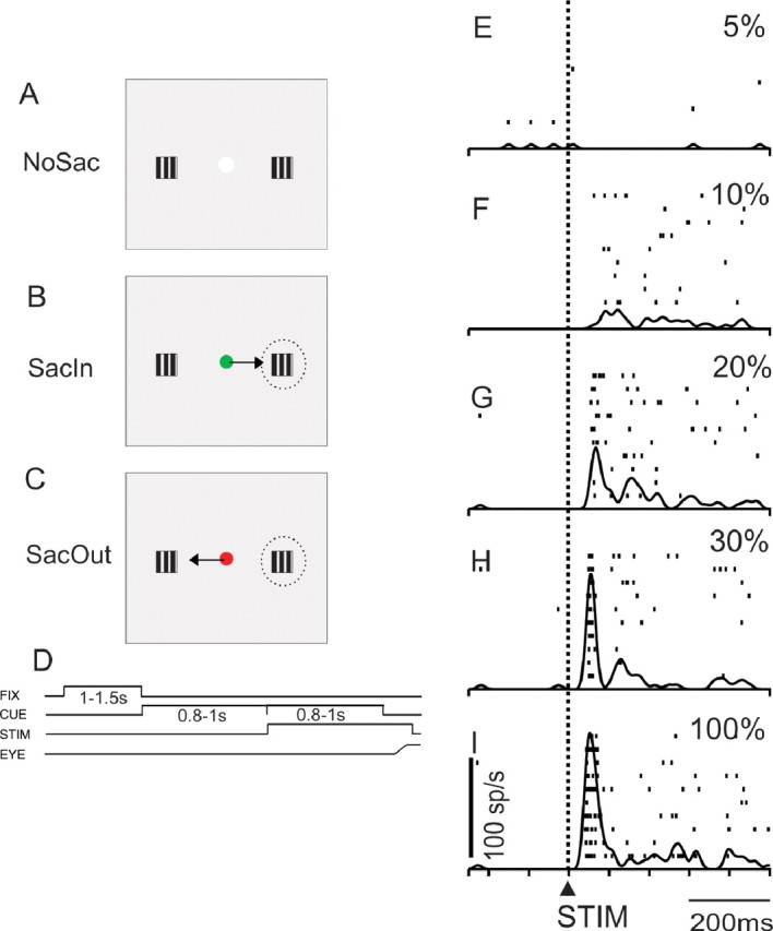
SC neurons respond to luminance gratings. A, Spatial depiction of the three conditions of the task. The gray square indicates the display at which the monkeys looked. Each hemifield contained a square-wave grating with varying contrasts. The centrally located spot (white) was the fixation point. NoSac indicates that the monkeys were required to remain fixating for the duration of the trial. B, Same as in A for the SacIn condition in which the monkey made a saccade to the RF. The green fixation point was a cue for these trials, and the arrow indicates the saccade direction. Dashed ovals are schematics of the RF. C, Same as in A and B for the SacOut trials. A red central cue indicated that a saccade out of the RF would be required. D, Temporal arrangement of the task. Upward deflection in the line indicates that the stimulus was turned on. Downward deflections indicate the stimulus was turned off. FIX, Fixation point; CUE, color change in fixation point; STIM, appearance of contrast patches; EYE, schematic of the eye position requirement of the task. E–I, A single SC neuron recorded in the NoSac condition. The dashed vertical line and upward arrow labeled STIM on the bottom panel indicate the alignment of the traces on the onset of the contrast patches. Each panel is taken from a set of trials for each contrast. The contrast relative to background is indicated as a percentage for each panel. Each tick is an action potential, and each row of ticks is a trial. The raster plots have the spike density function (σ = 10 ms) superimposed.

After the onset of a centrally located, white spot for a random time of 1000–1500 ms, the spot changed color to green or red, or remained white, for a random delay of 800–1000 ms. Monkeys were required to fixate this spot. Then, one luminance contrast patch was presented in the response field (RF) of a neuron while an identical luminance contrast patch was presented simultaneously in the mirror location in the other hemifield. After another 800–1000 ms delay, the centrally located cue disappeared if it was green or red, or it remained illuminated if it was white. The disappearance of the green or red cue was the signal for the monkey to make a saccade to the patch. If the central spot remained, monkeys remained fixating for 400–600 ms until receiving a fluid reward. Three conditions were used in this task. In the SacIn condition, monkeys made saccades to the RF. In the SacOut condition, monkeys made saccades to the location 180° away from the RF. In the NoSac condition, monkeys maintained fixation on the center spot (see Fig. 1A–D). The trial conditions (SacIn, SacOut, or NoSac) were presented in blocks that varied in order from day to day. The different luminance contrasts of the visual stimuli appeared 15–20 times in each block and were randomly interleaved within a block. Therefore, monkeys could predict whether or not a saccade would be required as well as the location of the upcoming saccade, but they could not predict the contrast of the upcoming stimulus.

Data acquisition.

Using the magnetic induction technique (Fuchs and Robinson, 1966) (Riverbend Instruments, Birmingham, AL), voltage signals proportional to horizontal and vertical components of the position of one eye were filtered (eight-pole Bessel, −3 dB, 180 Hz), digitized at 16-bit resolution, and sampled at 1 kHz (CIO-DAS1602/16; Measurement Computing, Norton, MA). The eye position data were saved for off-line analysis using an interactive computer program designed to display and measure eye position and calculate eye velocity. We used an automated procedure to define saccadic eye movements by applying velocity and acceleration criteria of 20 °/s and 8000 °/s², respectively. The adequacy of the algorithm was verified on a trial-by-trial basis by the experimenter. Single neurons were recorded with tungsten microelectrodes (Frederick Haer, Bowdoinham, ME) with impedances between 0.3 and 1.0 MΩ measured at 1 kHz. Electrodes were aimed at the SC through stainless steel guide tubes held in place by a plastic grid secured to the cylinder (Crist et al., 1988). In real time, action potential waveforms were identified with a window discriminator (Bak Electronics, Mount Airy, MD) that returned a TTL pulse for each waveform that met amplitude and voltage criteria. The TTL pulses were sent to a digital counter (PC-TIO-10; National Instruments, Norton, MA) and were stored to disk with a 1 ms resolution.

Neuronal classification.

We assessed the center of the RF of SC neurons empirically by listening for the maximal neuronal discharge as a spot of light was moved around the visual screen and monkeys maintained fixation on a centrally located spot. We also assessed the center of the movement fields of neurons by having monkeys make saccades to different regions of the visual field. In general, the centers of the receptive and movement fields were aligned. Because we placed the luminance grating in the same location for all task conditions for each recorded neuron and made comparisons across trial conditions (within design), asymmetries between field centers, if present, would not impact the results or conclusions. The diameter of the RFs of all SC neurons recorded was >6°. Seventy-three of 79 neurons had RF centers >5°. Six of 79 had RF centers between 3 and 5°.

We classified neurons as buildup, visual motor, visual tonic, and visual phasic using the following statistical criteria. We computed a baseline interval (mean discharge rate −200 to 0 ms from the onset of the luminance gratings but after the appearance of the color cue), a visual interval (0–200 ms beginning at the appearance of the luminance gratings), a delay interval (300–800 ms after the onset of the luminance gratings), and a saccade interval (−50 to 0 ms from the saccade onset). Using only correct trials, we defined buildup neurons as those neurons with at least 30 spikes (sp)/s discharge during the delay interval (Munoz and Wurtz, 1995) and significantly greater activity in the delay interval compared with the baseline (t test, p < 0.05) as well as significantly greater activity (t test, p < 0.05) in the saccade interval compared with the delay interval similar to the criteria used by us and others previously (Edelman and Keller, 1998; Paré and Wurtz, 2001; McPeek and Keller, 2002; Li and Basso, 2005; Li et al., 2006). Visual motor neurons had no significant delay activity compared with the baseline. If a neuron had a visual response and a significantly greater level of activity in the delay interval than the baseline interval (t test, p < 0.05) but had no significant difference in activity between the saccade and delay intervals, we classified the neuron as visual tonic. If a neuron had only a visual response but no significant delay and saccade interval activities, we classified it as visual phasic.

Data analysis: C₅₀ and receiver operating characteristic analysis.

Statistical analyses and curve fits were performed using Matlab 6.5.1 (MathWorks, Natick, MA). Standard parametric, descriptive, and inferential (ANOVA, t tests with modified Bonferroni's corrections) statistics were used (Keppel, 1991). If the data failed to pass normality tests, nonparametric statistics (Wilcoxon's test signed rank, rank sum, or Mann–Whitney U with modified Bonferroni's corrections) were used.

One way we tested neuronal sensitivity to contrast and changes associated with trial conditions was by assessing the C₅₀ parameter of fits of hyperbolic ratio functions to the neuronal discharge measured with different luminance contrast stimuli. To determine the C₅₀ parameter, contrast–response data were fitted with hyperbolic ratio functions of the following form: r = R_max (Cⁿ/(C + C₅₀ⁿ)) + m, using a nonlinear least-squares optimization procedure (Matlab 6.5.1; MathWorks), where R is the neuronal response, C is the contrast, R_max is the response amplitude between the upper and lower asymptotes, m is the postcue baseline activity (lower asymptote), C₅₀ is the contrast at which the neuronal response is halfway between the upper and lower asymptotes (also referred to as the semisaturation contrast), and n is an exponent that determines the steepness of the response function. In the actual fitting process, we subtracted the postcue baseline discharge from the visual responses first and then set m to 0. To determine how well the model fit the data, we computed the percentage of variance explained by the model fits (Carandini et al., 1997; Heuer and Britten, 2002). Only neurons passing a >60% variance explained criterion are presented in the analyses (see Fig. 6E,F). To determine the significance of differences between parameters of the hyperbolic functions, we applied a bootstrapping procedure. We first shuffled the trials for each contrast independently (at least 10 trials per contrast) using randperm() (Matlab 6.5.1; MathWorks). We then selected one trial for each contrast by choosing the first row of data points. This resulted in one sample set. The sample set was fitted with the hyperbolic ratio function, and the parameters were measured. We then shuffled the trials for each contrast again and reselected one trial from each contrast, again from the first row of data points. This procedure was repeated 1000 times to generate a distribution of function parameters. We then performed Wilcoxon's tests between the function parameters from each of the trial conditions (SacIn, NoSac, and SacOut). Table 1 reports the numbers of neurons with statistically significant changes in C₅₀ values for the saccade cue conditions.

Figure 6.

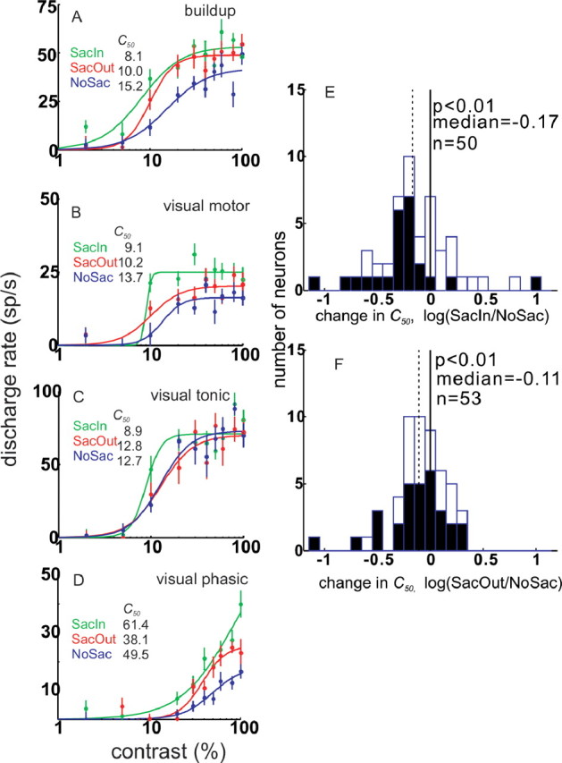
SC contrast response functions vary with cueing condition. Four example SC neurons are shown. Green circles and lines are data and fitted hyperbolic functions for the SacIn condition. Red circles and lines are data and fitted hyperbolic functions for the SacOut condition. Blue circles and lines are data and fitted hyperbolic functions for the NoSac condition. Each circle is the mean of at least 10 trials. The vertical bars through the circles are 1 SE. In each panel, the activity measured from 0 to 100 ms after the onset of the luminance grating is plotted in spikes per second against contrast on a logarithmic axis. The baseline neuronal activity was subtracted. A, The initial 100 ms of visual activity is plotted for one example buildup neuron. B, The initial 100 ms of visual activity is plotted for one example visual motor neuron. C, The initial 100 ms of visual activity is plotted for one example visual tonic neuron. D, The initial 100 ms of visual activity is plotted for one example visual phasic neuron. E, Frequency distribution of the number of neurons and the changes in the C₅₀ parameter as evaluated by taking the log of the ratio of the SacIn and NoSac C₅₀ values. The solid vertical line indicates 0 or no change in the two conditions. The dashed vertical line shows the median change in the C₅₀ parameter in the SacIn versus the NoSac conditions. Filled bars indicate statistically significant changes in C₅₀, whereas open bars indicate neurons with no significant change in C₅₀. F, The same as in E for the SacOut versus the NoSac conditions.

Table 1.

C₅₀ analysis

Neuron type	Number	SacIn versus NoSac
		<	>
Total	79	21 (26.6)	2 (2.5)
Buildup	31	9 (29.0)	1 (3.2)
Visual motor	30	6 (20.0)	1 (3.3)
Visual tonic	11	5 (45.5)	0 (0)
Visual phasic	7	1 (14.3)	0 (0)

Changes in C₅₀ with a cue to make a saccade. The total number of SC neurons is shown in the column titled Number. The numbers of neurons with a reduced C₅₀ in the SacIn condition compared to the NoSac condition are indicated by the number in the column marked <. Those showing increased C₅₀ in the SacIn condition are indicated in the column marked >. Percentages are indicated in parentheses. Only statistically significant differences are shown (Wilcoxon p < 0.05). Note that decreases in C₅₀ indicate increases in neuronal sensitivity. See Materials and Methods for details on how C₅₀ was determined. Of the 79 neurons in our sample, 50 of the neuronal CRFs were well fit with hyperbolic functions in both the SacIn and NoSac conditions (see Materials and Methods). Of these, 21 of 50 (42.0%; 21 of 79 = 26.6%) showed decreases in C₅₀ (Wilcoxon, p < 0.05), indicating an increase in sensitivity with a cue to make a saccade.

To estimate the ability of neurons to detect luminance contrast and provide a second way to assess neuronal sensitivity to luminance contrast, we performed receiver operating characteristic (ROC) analysis using the data from neuronal spike density functions (σ = 10 ms). To ensure that the width of the Gaussian used to convolve the spike train data did not skew our results, we performed an analysis on a random set of 14 neurons collapsed over nine contrasts. We computed the ROC curves (as described below) for the data with σ = 10 ms, σ = 8 ms, and σ = 4 ms, values that are used typically for SC neuronal data. In net, halving the width of the Gaussian reduced the ROC area by ∼7%. Importantly, because we made comparisons of ROC areas across trial conditions, the slight differences in ROC areas computed with different σ values do not alter the results or conclusions.

ROC curves and areas were computed by comparing the initial visual response (0–100 ms from the onset of the luminance gratings) of a neuron with its baseline activity. We used 200 ms of baseline activity measured before the appearance of the luminance gratings but after the color change of the central spot (postcue baseline activity). We computed the probability that the discharge rate exceeded a criterion for the measurement epoch in step sizes of (maximum − minimum discharge rate/100). A single point on the ROC curve was produced for each increment in the criterion, and the entire ROC curve was generated from all the criteria. The area under the ROC curve, therefore, measures the separation between two probability distributions. One distribution is the discharge rates of the stimulus-evoked visual activity and the second is the discharge rates measured for baseline. This analysis provides a way to measure the ability of a neuron to detect the presence of a stimulus in its RF. Differences in ROC area values across trial conditions indicate changes in neuronal detectability. Wilcoxon's rank sum test was used to assess statistical significance between cueing conditions across the sample of neurons (NoSac, SacIn, and SacOut).

In addition to comparing ROC areas between contrasts and conditions for all neurons, we also compared the area under the ROC across all contrasts and all conditions for individual neurons to determine the sensitivity to contrast in the different task conditions (Bradley et al., 1987; Reynolds et al., 2000; Li and Basso, 2005). We fitted the ROC values with a Weibull function of the form f(x) = L + (U − L)(1 − 2^−(x/α)β) using a nonlinear least squares optimization procedure (Matlab 6.5.1; MathWorks), where f(x) is the fit to the ROC values, x is the luminance contrast, L is the lower asymptote of the fitted curve, U is the upper asymptote, α is the contrast at which the function reaches its halfway point between L and U, and β determines the slope of the function. We set L to 0.5 because ideally a neuron cannot detect 0% contrast. The α parameter was used to quantify the sensitivity of neurons to contrast (also referred to as contrast threshold by Reynolds et al., 2000), and differences between α parameters measured between conditions was used to quantify the change of neuronal sensitivity. To determine how well the Weibull function fit the data, we computed the percentage of variance explained by the model fits (Carandini et al., 1997; Heuer and Britten, 2002). Only neurons passing the >60% criterion are presented in this analysis (see Fig. 9B,C). To determine the significance of differences between α parameters of the Weibull functions, we applied a bootstrapping procedure (see above) and created 1000 samples. Each sample was then fitted with the Weibull function and the parameters measured. We then performed Wilcoxon's tests between α parameters from each of the trial conditions across the sample of neurons (SacIn, NoSac, and SacOut). Table 2 reports the numbers of neurons with statistically significant changes in α parameter values for the different saccade cue conditions.

Figure 9.

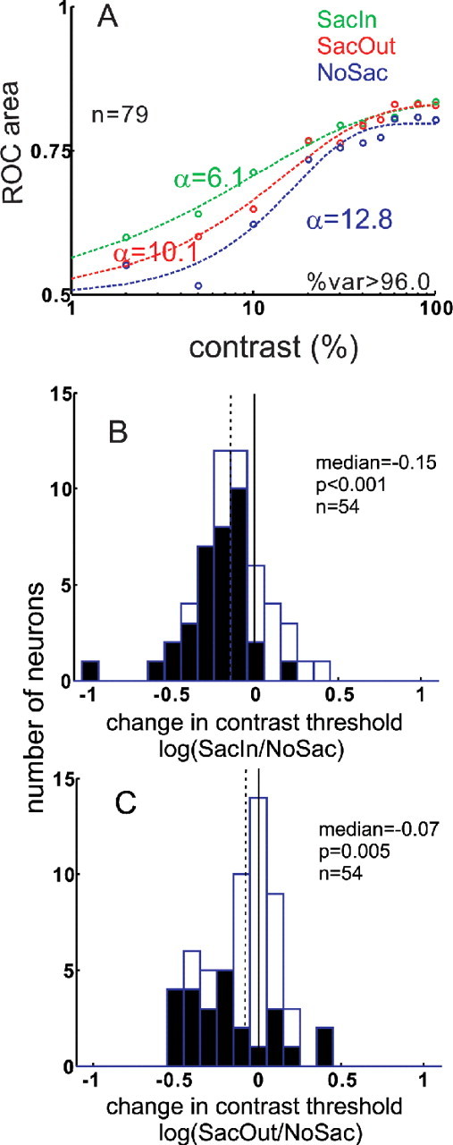
Saccade cue condition alters SC neuronal sensitivity to contrast. A, ROC area values are plotted against contrast condition for the three cueing conditions: blue circles, NoSac; green circles, SacIn; and red circles, SacOut for all 79 SC neurons. The dashed lines illustrate the best fitting Weibull functions through the data points (see Materials and Methods). The α parameter of Weibull function indicates the contrast threshold for the neurons. B, Change in the contrast threshold was determined by taking the log of the ratio of SacIn to NoSac α parameters. Filled bars indicate statistically significant changes in the α parameter (Wilcoxon's test, p < 0.001). The median change in α parameter was −0.15. C, Same as in B for the SacOut trial condition. The median change in the α parameter was −0.07. In both B and C, only the 54 of 79 neurons that were well fit with Weibull functions in both conditions are shown. In both B and C, solid vertical lines indicate no change, whereas the dashed vertical lines indicate the change in the contrast threshold.

Table 2.

ROC analysis: α parameter

Neuron type	Number	SacIn versus NoSac
		<	>
Total	79	32 (40.5)	3 (3.8)
Buildup	31	16 (51.6)	1 (1.3)
Visual motor	30	11 (36.7)	2 (6.7)
Visual tonic	11	5 (45.5)	0 (0)
Visual phasic	7	0 (0)	0 (0)

Changes in Weibull function α parameter with a cue to make a saccade. The total number of neurons is shown in the column titled Number. The numbers of neurons with significantly decreased α parameters across all contrast conditions are indicated by the number in the column marked <. Those showing increased α parameter are indicated by >. Percentages are indicated in parentheses. Only statistically significant differences are shown (Wilcoxon p < 0.05). Note that decreases in the α parameter indicate increases in sensitivity. See Materials and Methods for details of ROC analysis and how the α parameter was determined. Fifty-four of 79 of the neuronal ROC areas were well fit with Weibull functions in both the SacIn and NoSac conditions. Of these, 32 of 54 (59.2%; 32 of 79 = 40.5%) showed decreases in the α parameter (Wilcoxon p < 0.05).

Results

Trained monkeys prepared to make or withhold saccades in response to the color of a cue located at the center of a visual screen (Fig. 1). After the central cue appeared, two square-wave, luminance gratings appeared. One was located in the RF of a neuron recorded from the SC. The second was located in the visual field 180° opposite to the RF. The luminance gratings varied in contrast from low (2%) to high (100%), defined as (L_h − L_l)/(L_h + L_l), where L_h is the highest luminance, and L_l is the lowest luminance (DeValois and DeValois, 1990). We recorded 79 neurons from four SCs of two monkeys and classified each as buildup (n = 31), visual motor (n = 30), visual tonic (n = 11), or visual phasic (n = 7; see Materials and Methods). The different color cue conditions were presented in ordered blocks that varied across days. The luminance contrasts of the stimuli appeared randomly within blocks. With this arrangement, monkeys could predict whether or not a saccade would be required and where the saccade would be located, but they could not predict the contrast of the target (Fig. 1A–D).

Luminance contrast modulates SC neuronal activity

Figure 1E–I shows the activity of an example SC neuron recorded during the presentation of different luminance contrast gratings that appeared within an SC RF. In this example, the monkey maintained fixation on the central spot (NoSac). At low contrasts, there was very little response from the SC neuron (Fig. 1E,F). Not altogether surprising, as the contrast increased, the sensory activity of the SC neuron became more vigorous (Fig. 1G–I).

The pattern of increasing discharge with increases in luminance contrast was evident for all SC neuron types recorded. Figure 2 shows the discharge rate of four example SC neurons plotted for the different contrasts with baseline subtracted. With a 2% contrast stimulus in the RF, little sensory discharge appeared in buildup neurons (Fig. 2A), visual motor neurons (Fig. 2B), and visual tonic neurons (Fig. 2C). Visual phasic neurons showed little response to 2% contrast patches (Fig. 2D). As luminance contrast increased up to 100%, all SC neuron types showed increased discharge (Fig. 2A–D).

Figure 2.

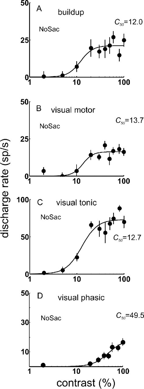
Contrast–response functions of monkey SC neurons. The mean neuronal discharge rate (spikes per second) measured 0–100 ms after the onset of the luminance contrast stimuli is plotted against increasing percentage contrast of the stimuli from the NoSac trial condition. Each circle is the mean of at least 10 trials, and the vertical line on each circle is 1 SE. The line connecting the circles is the best fitting hyperbolic function (see Materials and Methods). A, Example buildup neuron data. B, Example visual motor neuron. C, Example visual tonic neuron. D, Example visual phasic neuron. Baseline activity measured 200 ms after the appearance of the cue but before the appearance of the luminance patches was subtracted from the data.

To quantify the pattern of responding across all neurons in our sample, we computed the mean and SE of the discharge rate for the visual response (0–100 ms after the luminance grating onset) in the NoSac condition across all trials for all neurons and for each of the 10 contrast stimuli presented (Fig. 3A). The baseline discharge rate (200 ms interval before luminance grating onset and after the color cue appearance) was subtracted from the stimulus-evoked discharge. These contrast–response functions (CRFs) reveal that the visual response of all SC neuron types increased as luminance contrast increased. Visual phasic neurons seemed to require a higher stimulus contrast to drive them compared with the other neuron types (Fig. 3A, squares). As a first step toward determining whether this apparent difference in responding of visual phasic neurons was consistent, we fitted the mean of the sample of data from each of the neuron types with hyperbolic ratio functions and measured the C₅₀ from each (Fig. 3A). We found that the C₅₀ for visual motor neurons was 15.2% (Fig. 3A, cyan). The C₅₀ for buildup neurons was 18.1% (Fig. 3A, red). From the visual tonic neurons, we obtained a C₅₀ of 12.9% (Fig. 3A, green). The C₅₀ measured from the visual phasic neurons was 24.1%. This increase in semisaturation contrast indicates a lower sensitivity to contrast of visual phasic neurons compared with the other neuron types of SC. Consistent with this observation, we found that, when the hyperbolic ratio function was fit to the contrast–response functions for individual neurons (Fig. 3B), the median values of C₅₀ obtained ranged from 18.2 to 34.5, and the visual phasic neurons tended to have the highest C₅₀ values (Fig. 3B).

Figure 3.

Luminance contrast modulates SC neuronal activity. A, The mean neuronal discharge rate (spikes per second) during the initial visual interval (0–100 ms after luminance contrast patch onset) for all 79 neurons is plotted as a function of percentage contrast on a logarithmic axis. Baseline discharge was subtracted. The mean responses for each neuron type are shown as different symbols and colors. The vertical bars are 1 SE. The lines through the data points are the best fit hyperbolic ratio function (see Materials and Methods). The dashed vertical line and the corresponding value indicate the C₅₀ or semisaturation constant of the function. Visual motor neuronal data are shown in cyan upward triangles. Visual tonic neuronal data are shown in green rightward-facing triangles. Buildup neuronal data are the red circles, and visual phasic neuronal data are the purple squares. n indicates the number of neurons for each type. B, The frequency distribution of the C₅₀ parameters obtained for individual SC neurons. The inset values indicate the median C₅₀ parameter across the SC neuron types. The color scheme is the same as in A.

We also assessed the contrast responding of visual phasic neurons compared with the other SC neuron types using ROC analysis and obtained a similar result. This is described in supplemental Figure 1 (available at www.jneurosci.org as supplemental material). One possible explanation for the lower contrast sensitivity of visual phasic neurons compared with the other SC neuron types may be the relatively smaller RF size of these neurons (Goldberg and Wurtz, 1972a; Wurtz and Mohler, 1976; Munoz and Wurtz, 1995). This explanation has been suggested for differences in contrast sensitivity of visual cortical neurons (Sclar et al., 1990). Because we have no additional data to address this, we leave this point here.

Saccade selection and preparation influence sensory responses in SC: discharge rates

Providing cues to move the eyes to a location influenced the initial visual response of SC neurons to the luminance contrast patches. Figure 4A–D shows the activity of the sample of 79 SC neurons across three of the contrasts for the different task conditions. The mean baseline discharge of the neurons was subtracted on a neuron by neuron basis. The four SC types are presented separately. Mean spike density functions are plotted for the NoSac condition (Fig. 4A–D, blue traces), for the SacIn condition (Fig. 4A–D, green traces), and for the SacOut condition (Fig. 4A–D, red traces). Compared with the NoSac condition, the responses of SC neurons to the same visual stimuli were larger when a cue to make a saccade to the RF appeared (Fig. 4A–C, leftmost panels, compare green and blue traces). This is not surprising by itself because SC neurons are known to have enhanced responses for visual stimuli that are likely to become saccade targets (Goldberg and Wurtz, 1972b; Wurtz and Mohler, 1976; Basso and Wurtz, 1997, 1998; Dorris and Munoz, 1998). What was surprising here was that, first, the enhancement appeared with a cue to make a saccade, well before the saccade occurred. The original description of enhancement referred to the increase in sensory discharge that occurred coincident with saccade occurrence (Goldberg and Wurtz, 1972b; Wurtz and Mohler, 1976). Second, the increase in sensory discharge was apparent for neurons with saccade-related activity. The original enhancement experiments described increased responses only for sensory neurons, not movement neurons (Wurtz and Mohler, 1976). Third, the relative increase in discharge rate from the NoSac to SacIn conditions appeared more prominent for visual stimuli with lower rather than higher contrasts (Reynolds et al., 2000; Martinez-Trujillo and Treue, 2002) (Fig. 4, compare green and blue traces across columns). Finally, when a cue to make a saccade to the location opposite the RF was provided, SC neurons also appeared to have increased responses compared with the NoSac condition (Fig. 4, compare red and blue traces). This nonspatially selective increase in neuronal discharge was smaller than that seen in the SacIn condition (Fig. 4, compare red and green traces).

Figure 4.

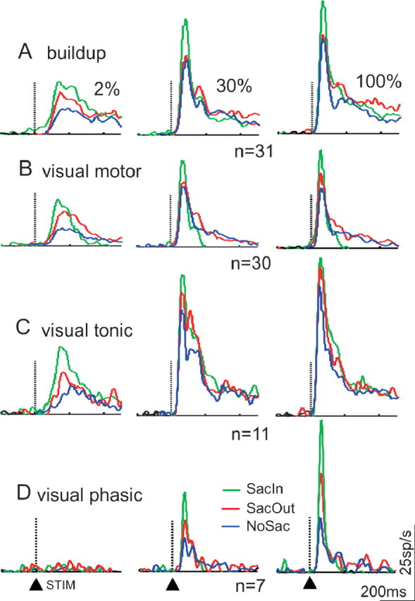
Cueing conditions modulate SC neuronal responses to luminance contrast. A, The neuronal discharge rates of the sample of SC buildup neurons for a subset of the contrasts: 2% (left column), 30% (middle column), 100% (right column). B, Same as in A for visual motor neurons. C, Same as in A and B for visual tonic neurons. D, Same as in A–C for visual phasic neurons. The dotted vertical line, arrowhead, and STIM (appearance of contrast patches) at the bottom of the panels indicate the alignment of each panel on the onset of the luminance gratings. In each panel, the green traces are the mean spike density functions (σ = 10 ms) measured for the sample of neurons in the SacIn condition. The red traces are the same for SacOut condition, and the blue traces are the same for the NoSac condition. n indicates the number of neurons in each group. The baseline activity was subtracted from the stimulus-driven and delay activity for each neuron.

To quantify the changes in discharge rate of SC neurons across task conditions, we could not compare the absolute discharge rates directly because the low discharge rate of neurons in the low-contrast conditions would skew the results. Therefore, we computed the ratio of the difference in activity in two conditions (with postcue baseline subtracted) divided by the sum of the activity in the same two conditions. The ratio was multiplied by 100 to be expressed as a percentage difference. This procedure is similar to that performed by Reynolds et al., 2000 (their Fig. 6), allowing a direct comparison with those results. Figure 5 shows frequency histograms of the number of neurons and the percentage difference in activity that occurred in the different saccade cueing conditions collapsed across all SC neuron types.

Figure 5.

Cueing conditions alter the visual discharge of SC neurons. The number of neurons is plotted against the percentage change in neuronal activity (spikes per second). % change = (SacIn − NoSac)/(SacIn + NoSac) × 100 is plotted in the column A for five contrast conditions: 2, 5, 10, 20, and 100%. % change = (SacOut − NoSac)/(SacOut + NoSac) × 100 in the column B for the same five contrast conditions. The neuronal discharge used for the calculation was the 0–100 ms interval after the onset of the luminance gratings with the baseline activity subtracted. Each panel shows the distribution of percentages for one contrast. The contrast is indicated in the rightmost column labeled “Contrast.” Although the experiment included 10 contrast levels, we show only five to maximize clarity. The percentage on the top right corner in each panel is the median percentage of enhancement of neuronal discharge between the two conditions. The long, thick vertical lines indicate 0% (no difference between conditions). The thin dashed vertical lines show the median percentage change. A black triangle by the thin dashed vertical line indicates that the percentage change was statistically significant for that stimulus contrast (Wilcoxon's test, p < 0.05). A gray triangle by the thin dashed vertical line indicates that the percentage change was not statistically significant for that stimulus contrast (Wilcoxon's test, p > 0.05).

A cue indicating a saccade into the RF generally resulted in an increase in the initial visual response of SC neurons compared with when a cue indicated no saccade (Fig. 5A). Similarly, a cue indicating a saccade out of the RF resulted in an increase in the initial visual response of SC neurons compared with a cue indicating no saccade (Fig. 5B), although the latter increase was not as large as the former increase (Fig. 5A, black triangle shifted farther rightward compared with the gray triangle in B). Comparing across all contrasts, we identified two main results. First, the trend of increasing discharge was evident across all contrasts but was larger for lower contrast stimuli. For example, when the luminance grating with 5% contrast appeared and monkeys were cued to make a saccade into the RF, there was a median 75.5% increase in discharge rate compared with when no saccade was required (Fig. 5A, black triangle in second row). The same comparisons for a higher contrast stimulus, for example 20%, revealed a similar but quantitatively smaller effect of task condition (median of 29.4% increase in discharge rate) (Fig. 5A, black triangle in fourth row). We combined the three lowest contrasts (2, 5, and 10%) as a low-contrast group and the three highest contrasts (60, 80, and 100%) as a high-contrast group. Then we compared the percentage difference in activity of the SacIn and NoSac conditions between these two groups. The percent difference between the low- and high-contrast groups was confirmed as statistically significant (Wilcoxon's test, p < 0.001). Thus, across the sample of SC neurons, increases in neuronal discharge rate with a cue to make a saccade into the RF were evident for all contrasts but were larger when the target stimulus had lower contrast. Note that the largest increase occurred for the second to lowest contrast. This result is consistent with the maximal effects occurring within the dynamic range of neurons.

The second result obtained from this analysis was that the increase in discharge also occurred when monkeys were cued to make saccades outside of the RF. For the 5% contrast condition, a direct comparison between the SacOut condition and the NoSac condition neuronal discharges revealed a 37.8% increase in discharge rate (Fig. 5B, black triangle in second row). For a target stimulus with 20% contrast, when a cue to make a saccade outside of the RF occurred, the discharge rate increased but only by 12.8% (Fig. 5B, black triangle in fourth row). Thus, although there were statistically significant increases in discharge rate associated with making a saccade outside of the RF (Fig. 5B, black triangles), the increases were quantitatively smaller (37.8 and 12.8%) than the increases associated with making a saccade into the RF (75.5 and 29.4%). The differences between the low- and high-contrast groups for the SacOut condition, however, were not statistically significant (Wilcoxon's test, p = 0.07). Together, these results indicate that a spatially selective signal and a smaller, nonspatially selective signal modulate SC neuronal responses. Furthermore, the spatially restricted modulations are more prominent for lower-contrast stimuli.

Do changes in discharge rate indicate changes in neuronal sensitivity?

Up to now, we showed that the initial visual discharge of SC neurons varied with different levels of luminance contrast. We also showed that the visual discharge of SC neurons in response to the presence of the same visual stimuli differed depending on whether the monkey saw a cue to make a saccade or not or whether the monkey saw a cue to make a saccade into or out of the RF. What we were most interested in, however, was whether SC neurons were more likely to detect the presence of a visual stimulus in their RF depending on the color cue or whether they had a reduced threshold for responding to a similar contrast with color cues. In other words, do SC neurons increase their detectability and sensitivity to luminance contrast when a cue to select and prepare a saccade appears?

To determine whether the increase in SC neuronal responses indicated a change in the ability of SC neurons to detect a stimulus in their RF and to determine whether SC neurons had an increase in sensitivity to luminance contrast, we performed two analyses. All analyses were applied to individual SC neurons as well as across the sample of SC neurons. First, we fit the neuronal discharge data across contrasts with a hyperbolic ratio function and measured the C₅₀ parameter from the function (see Materials and Methods). The C₅₀ parameter indicates the half-maximal rate of responding between the upper and lower asymptotes (Albrecht and Hamilton, 1982; Sclar et al., 1990; Williford and Maunsell, 2006). Changes in C₅₀ indicate changes in neuronal sensitivity to contrast. We assessed statistical significance of the C₅₀ parameter using a bootstrapping procedure.

For the second test, we performed ROC analysis on the initial visual discharge rate compared with the postcue baseline discharge rate of the neurons (see Materials and Methods). The same baseline measurement was used here as for the C₅₀ analysis. Because we compared the visual activity with the baseline activity after the color cue appeared, the ROC area provided a measure of detectability because it took into account any changes in nonstimulus-driven activity of the neurons resulting from the color cue. We assessed the ROC areas for individual neurons and across the sample of neurons in the different cue conditions and across contrasts. We determined statistical significance of the ROC areas using Wilcoxon's rank sum. We determined neuronal sensitivity to contrast by fitting the ROC areas across all stimulus contrasts with Weibull functions and determined the α parameter of the Weibull functions to measure contrast thresholds (Reynolds et al., 2000). Because the α parameter is a measure of neuronal responding across all contrasts, it provides a measure of neuronal sensitivity to luminance contrast. Using a bootstrapping procedure, we assessed the statistical significance of the changes in contrast threshold across trial conditions.

Saccade selection and preparation influence neuronal sensitivity to contrast: C₅₀

Figure 6A–D shows CRFs of four example SC neurons, one of each type. Each curve in each panel is the fitted hyperbolic ratio function to the neuronal discharge measured in the three cue conditions (green, SacIn; blue, NoSac; red, SacOut). Note that, like Figure 4, the postcue baseline discharge activity was subtracted from the sensory-evoked response. In each case, the CRF measured from the data obtained in the SacIn condition was shifted to the left compared with the CRF measured from the data obtained in NoSac condition (Fig. 6A–D, compare green and blue lines). For comparison, the C₅₀ values are provided for each condition as insets. Figure 6A shows an example buildup neuron recorded with different luminance contrast stimuli in the three cue conditions. The lines through the data points show the best fitting hyperbolic ratio function. The C₅₀ value is the stimulus contrast at which the neuron discharges at half of its maximal rate of responding. For this example neuron, the half-maximal response was obtained at 15.2% contrast in the NoSac condition (Fig. 6A, blue curve). In the SacIn condition, the half-maximal response was achieved when a stimulus with only 8.1% contrast appeared (Fig. 6A, green curve). There was an increase in the sensitivity of this neuron to contrast by 46.7% with a cue to select a saccade. Note that the SacOut condition fell between these two values (Fig. 6A, red curve) (C₅₀ of 10.0%; 34.2% increase in sensitivity compared with NoSac). A similar trend was observed for the visual motor neuron (Fig. 6B). The NoSac condition had a C₅₀ of 13.7%, whereas the SacIn condition C₅₀ was 9.1%. This was a 33.6% increase in sensitivity with a cue to make a saccade. For the example visual tonic neuron, the C₅₀ value in the SacOut condition was close to that in the NoSac condition (Fig. 6C), but the SacIn condition showed the same decrease as seen in buildup and visual motor neurons. The SacIn condition also yielded a leftward shift in the hyperbolic ratio function for the visual phasic neuron, but, in this example, the C₅₀ value was 61.4% for the SacIn condition compared with 49.5% for the NoSac condition. The failure to obtain a smaller C₅₀ for this example neuron is likely attributable to the poorer fitting of the ratio function to data of this neuron. Overall, these example results show that there was an increase in neuronal discharge rate for the same contrast stimuli when a saccade would be required compared with when monkeys remained fixating, and the leftward shift of the hyperbolic ratio function suggests an increase in neuronal sensitivity to contrast (Williford and Maunsell, 2006).

To assess whether the C₅₀ parameter of the hyperbolic ratio function changed with the saccade cue condition across our sample of SC neurons, we determined the CRFs for each neuron across all contrasts for each of the three cue conditions. The neuronal discharge data obtained for each contrast were then fitted with a hyperbolic ratio function as described in Materials and Methods. To display the results, we determined the change in the C₅₀ parameter by taking the log of the ratio of the C₅₀ parameters in two conditions. Negative values indicate that the C₅₀ parameter decreases, favoring higher sensitivity. Positive values indicate increases in the C₅₀ parameter favoring lower sensitivity (higher threshold). Shown in Figure 6E is the result for the SacIn and NoSac change. Figure 6F shows the change in C₅₀ parameter for the SacOut and NoSac conditions.

Across the sample of all SC neurons, the median C₅₀ in the NoSac condition was 22.8%, whereas the median C₅₀ in SacIn condition was 14.2%. This 8.6% reduction in C₅₀ with a cue to make a saccade into the RF was statistically significant across the sample of neurons (Wilcoxon's test, p < 0.01). When expressed as the log(SacIn/NoSac), the median change in the C₅₀ was −0.17. This reduction was also statistically significant (Fig. 6E) (Wilcoxon's test, p < 0.01). The C₅₀ in the NoSac condition was 22.8%, whereas C₅₀ in SacOut condition was 18.1%. This 4.7% reduction in C₅₀ with a cue to make a saccade out of the RF was statistically significant across the sample of neurons (Wilcoxon's test, p < 0.01). When expressed as the log(SacOut/NoSac), the median change in the C₅₀ was −0.11. This reduction was also statistically significant (Fig. 6F) (Wilcoxon's test, p < 0.01). The magnitude of the change in C₅₀ that occurred with the SacIn cue was larger than the magnitude of the change in C₅₀ that occurred with the SacOut cue across the sample of neurons (8.6 vs 4.7% and −0.17 vs −0.11), although this difference failed to reach statistical significance (Wilcoxon's test, p = NS).

Saccade selection and preparation influence neuronal sensitivity to contrast: ROC

We used ROC analysis as a way to assess the ability of SC neurons to detect the presence of a stimulus in their RF (Bradley et al., 1987; Britten et al., 1992). We also used ROC analysis as a second way, in addition to the C₅₀ analysis, to assess neuronal sensitivity to contrast (Reynolds et al., 2000). By comparing the initial visual response (0–100 ms after the onset of the luminance gratings) of a neuron to its baseline activity (−200 to 0 ms from the onset of the luminance gratings but after the cue, indicating where to look), the ROC analysis tells how well a neuron can detect the visual stimulus. We calculated ROC area for each neuron in each contrast and cue condition. Because we computed the ROC area for each neuron and across all contrasts and cue conditions, we could fit these data with Weibull functions, determine the α parameter of the function (contrast threshold), and, therefore, also determine whether sensitivity across task conditions changed.

We assessed the ability of SC neurons to detect the presence of a stimulus by examining the ROC area computed for all neurons across all contrasts. Figure 7 shows the ROC areas obtained from our sample of 79 SC neurons in the three cue conditions and for four example contrasts: 2, 5, 10, and 100%. Figure 7A shows the ROC curves for the different contrast conditions. Not surprisingly, as the contrast of the stimulus increased, the ROC area also increased, consistent with an increased likelihood of detection. To quantify this, we grouped the ROC areas from the individual neurons into two contrasts groups, a low group and a high group. The low-contrast group comprised the 2, 5, and 10% contrasts, and the high-contrast group comprised the 60, 80, and 100% contrasts. Figure 7B illustrates the distribution of ROC areas in the two groups in the NoSac condition. Again, not surprisingly, the distribution of ROC areas was lower and more variable with lower-contrast stimuli (Fig. 7B, open bars), whereas the distribution of ROC areas was higher and less variable with higher-contrast stimuli (Fig. 7B, filled bars). The median ROC area for the neurons in the NoSac condition for the low-contrast group was 0.57 (Fig. 7B, dotted blue line). The median ROC area for the neurons in the NoSac condition for the high-contrast group was 0.84 (Fig. 7B, dashed blue line). These ROC areas differed significantly (Wilcoxon's test, p < 0.001). With a cue to make a saccade, ROC area increased (Fig. 7C). Across the sample of 79 neurons, there was a rightward shift of the distribution of ROC areas measured primarily in the low-contrast group (Fig. 7B,D, open bars). The median ROC area for the neurons in the SacIn condition for the low-contrast group was 0.68 (Fig. 7D, dotted green line), whereas for the high-contrast group the median ROC area was 0.85 (Fig. 7D, dashed green line). The differences in ROC area for the low-contrast groups in the SacIn and the NoSac conditions were statistically significant (Wilcoxon's test, p < 0.001). There was also an increase in ROC area for the different contrast targets with a cue to make a saccade out of the RF (Fig. 7E), although the increase in area did not appear as large as that seen with a cue to make a saccade into the RF. Across the sample of neurons, the ROC areas for individual neurons in the low-contrast group shifted slightly to the right in the SacOut condition compared with the NoSac condition (Fig. 7B,F, open bars). The median ROC area in the low-contrast group was 0.61 for the SacOut condition (Fig. 7F, dotted red line). The high-contrast group remained unchanged. The median ROC area was 0.84 (Fig. 7F, dashed red line). Together, the increase in ROC area across the sample of 79 neurons as well as for individual neurons indicates that the ability of SC neurons to detect a visual stimulus increases with a cue to make a saccade. Furthermore, a cue to make a saccade into the RF has a larger influence on detectability than a cue to make a saccade out of the RF.

Figure 7.

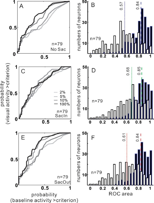
ROC area increases with cueing conditions. A, The probability of the initial visual activity exceeding criterion is plotted against the probability of the baseline activity exceeding criterion in the NoSac condition for all 79 SC neurons (for ROC curve calculation, see Materials and Methods). B, Distribution of ROC areas from all 79 neurons in the NoSac condition. C, Same as in A for the SacIn condition. D, Same as in B for the SacIn condition. E, Same as in A and C for the SacOut condition. F, Same as in B and D for the SacOut condition. In A, C, and E, the lines increasing in darkness correspond to ROC curves measured from trials with increasing in contrast. Light gray lines are from the 2% trials. Medium gray lines are from the 5% trials. Dark gray lines are from the 10% trials, and the black lines are from the 100% contrast trials. In B, D, and F, open bars are from the low-contrast group of trials (2, 5, and 10%). Filled bars are from the high-contrast group of trials (60, 80, and 100%). The dotted vertical dashed lines show the median ROC area obtained from the group of low-contrast conditions. The dashed vertical lines show the median ROC area obtained from the group of high-contrast conditions. Blue, NoSac; green, SacIn; red, SacOut.

In a second analysis, we plotted the ratio of ROC areas obtained in the SacIn to NoSac and SacOut to NoSac trial conditions expressed as a percentage for all the neurons. Figure 8 shows this for a subset of five contrast conditions in the form of histograms. The arrangement of these panels is the same as in Figure 5, A and B. Consistent with the trend seen in the discharge rates (Figs. 4, 5), the modulation of ROC area was most evident for stimuli with low contrasts. Comparing the difference in ROC area between the SacIn and NoSac conditions (Fig. 8A), the largest changes appeared in conditions in which stimuli had 2, 5, or 10% contrast (11.7, 23.1, and 12.8% increases, respectively). Significantly different modulations were observed between the SacIn and NoSac conditions for 2, 5, and 10% contrast stimuli (Fig. 8A, black triangles) (Wilcoxon's test p < 0.05). The results indicate that a spatially selective increase in detectability of luminance contrast occurs with a cue to make a saccade into the RF. The lower increase in detectability that occurred for high-contrast stimuli is not because the neurons are saturated at higher contrasts. For example, the neuronal discharge for the 30% contrast stimulus is less than the discharge for the 100% contrast stimulus (Fig. 4, middle and rightmost columns). This indicates that the neuronal response for a stimulus with 30% is not saturated. Therefore, it is unlikely that a stimulus with <30% contrast would drive the neuronal activity to saturation. We show, however, that the neuronal detectability measured with a stimulus that had a 20% contrast did not change much (Fig. 8A). Thus, if the only reason the changes were more apparent in the low-contrast conditions was because the neurons were discharging below saturation, we should have seen increases in detectability even in the 20% condition. But we did not.

Figure 8.

Saccade cue condition increases ROC areas. The ratio of ROC areas obtained in the SacIn condition to the NoSac condition multiplied by 100 provides an index of the percentage change in ROC area with a cue to select and prepare a saccade into the RF. The ratio of ROC areas obtained in the SacOut condition to the NoSac condition multiplied by 100 provides an index of the percentage change in ROC area with a cue to select and prepare a saccade out of the RF. Column A shows the SacIn/NoSac ratio, and column B shows the SacOut/NoSac ratios. Each row of two panels shows the result for a different contrast condition. Only 5 of the 10 contrasts were selected for display to minimize clutter. The arrangement is similar to that shown in Figure 5. The long, thick vertical lines indicate 100% (no difference between conditions). The thin, dashed vertical lines indicate the median percentage change in ROC area. A black triangle by the thin, dashed vertical line indicates that the percentage change was statistically significant for that stimulus contrast (Wilcoxon's test, p < 0.05). A gray triangle by the thin, dashed vertical line indicates that the percentage change was not statistically significant for that stimulus contrast (Wilcoxon's test, p > 0.05).

Interestingly, we also found that, for some contrasts, the SacOut condition was associated with higher neuronal detectability compared with the NoSac condition, although overall the changes were variable and small. For example, with 5% stimulus contrast, the SacOut and NoSac conditions showed a difference in ROC area (Fig. 8B). The area was 18.3% greater for the SacOut compared with the NoSac condition. This increase in ROC area was statistically significant (Wilcoxon's test p < 0.05). A small increase was observed for the 20% contrast stimulus (3.5%; Wilcoxon's test, p < 0.05) (Fig. 8B). Although quantitatively smaller than the changes seen in the SacIn versus the NoSac condition, the finding of an increase for the SacOut condition suggests that there is also a nonspatially selective enhancement of detectability when a saccade out of the RF is cued.

In addition to assessing neuronal detectability, we assessed neuronal sensitivity to stimulus contrast using the α parameter of the Weibull function fitted to ROC areas across all contrasts (see Materials and Methods). Figure 9A illustrates the mean of the ROC areas obtained for all 79 SC neurons as a function of contrast. Each of the three differently colored points shows the data for the three different cue conditions. Each of the three differently colored lines shows the fitted Weibull functions. The α parameter of the Weibull function indicates the half-maximal of the ROC area and, therefore, is similar to the C₅₀ of the hyperbolic function. Thus, the α parameter provides a measure of the sensitivity of the neuron to contrast. This parameter has also been referred to as the contrast threshold (Reynolds et al., 2000).

When considered as a measure of contrast threshold, the α parameter can also be used to assess changes in SC neuronal activity in terms of units of contrast, as had been done previously for V4 neurons (Reynolds et al., 2000). Across the sample of SC neurons, the α parameter measured in the NoSac condition was 12.8% contrast. Presenting a cue to make saccade into the RF compared with a cue to remain fixating changed the α parameter from 12.8 to 6.1%. This leftward shift of the neurometric function is equivalent to a 52.3% decrease in contrast threshold across the sample of neurons. The SacOut condition was associated with a small but reliable decrease in contrast threshold. The leftward shift of the SacOut curve compared with the NoSac curve was from 12.8 to 10.1%. The shift of the neurometric function in the SacOut condition is equivalent to 21.1% decrease in contrast threshold. Thus, a cue to make a saccade into the RF is associated with ∼50% increase in the neuronal sensitivity to contrast in SC visual responses. A cue to make a saccade out of the RF is associated with ∼20% increase in neuronal sensitivity. Tables 1 and 2 show a breakdown of the two sensitivity measures, C₅₀ and the α parameter obtained across the different SC neuron types. Of the total 79 neurons in our sample, 50 of the neuronal CRFs were well fit with hyperbolic functions in both the SacIn and NoSac conditions (see Materials and Methods). Twenty-one of 50 (42%; 21 of 79 = 26.6%) showed decreases in C₅₀ (Wilcoxon's test, p < 0.05), indicating an increase in sensitivity with a cue to select and prepare a saccade. Fifty-four of 79 of the neuronal ROC areas were well fit with Weibull functions in both the SacIn and NoSac conditions (see Materials and Methods). Of these, 32 of 54 (59.2%; 32 of 79 = 40.5%) showed decreases in the α parameter of the Weibull function (Wilcoxon's test, p < 0.05), indicating an increase in sensitivity with a cue to select and prepare a saccade.

As we did for the C₅₀ analysis, we computed the log of the ratio of the α parameters measured in the SacIn to NoSac conditions and the SacOut to NoSac conditions to quantify the change in contrast threshold with the three cueing conditions. Negative values indicate that the α parameter decreases, favoring higher sensitivity. Positive values indicate increases in the α parameter favoring lower sensitivity (higher threshold). Figure 9, B and C, illustrates the results for the 54 of 79 neurons that were well fit with Weibull functions. For the SacIn conditions, the median change in contrast threshold was −0.15. This decrease in threshold was statistically significant (Wilcoxon's test, p < 0.001). For the SacOut condition, the median decrease in threshold was −0.07. This decrease was also statistically significant (Wilcoxon's test, p < 0.001). The magnitude of the change in α parameter occurring with the SacIn cue was larger than the magnitude of the change in α parameter occurring with the SacOut cue across the sample of neurons (−0.15 vs −0.07). These differences were statistically significant (Wilcoxon's test, p < 0.01), consistent with a larger spatially selective increase in neuronal sensitivity to contrast and a smaller nonspatially selective increase in neuronal sensitivity to contrast. Note that, with the C₅₀ analysis, a similar trend was observed, but the difference between the SacOut and SacIn conditions failed to reach statistical significance. We suspect this occurred because ROC analysis is more sensitive than the C₅₀ parameter analysis.

Dynamics of neuronal sensitivity to contrast in SC

Figure 10A shows the average ROC area calculated from 0 to 600 ms for all 10 contrasts for all 79 SC neurons. Each line on the contrast–ROC plane is the neurometric function showing neuronal sensitivity to contrast. ROC area was computed for the first 100 ms interval of neuronal discharge measured in the NoSac condition compared with the postcue baseline discharge measured in the NoSac condition. In 50 ms steps, we advanced the 100 ms interval forward in time and recomputed the ROC area values for each contrast condition. We then interpolated the points along the time axis every 10 ms for smoothing. We also interpolated along the contrast axis every 1.0% contrast. The first curve on the contrast–ROC plane is the neurometric function from 1 to 100 ms after the luminance gratings appeared. The second curve is the neurometric function from 11 to 110 ms after the luminance grating appeared. The third curve is the neurometric function from 21 to 120 ms after the gratings appeared and so on. Figure 10B shows the same for the SacIn trial condition, and Figure 10C shows the same for the SacOut trial condition. Figure 11A–C shows the ROC areas calculated in the same way as in Figure 10, but here they are calculated backward in time, from the time of saccade onset (0 ms) to 850 ms earlier. Together, these two figures provide the complete time course of the changes in neuronal sensitivity to luminance contrast of SC neurons from the onset of the targets to the onset of the saccade.

Figure 10.

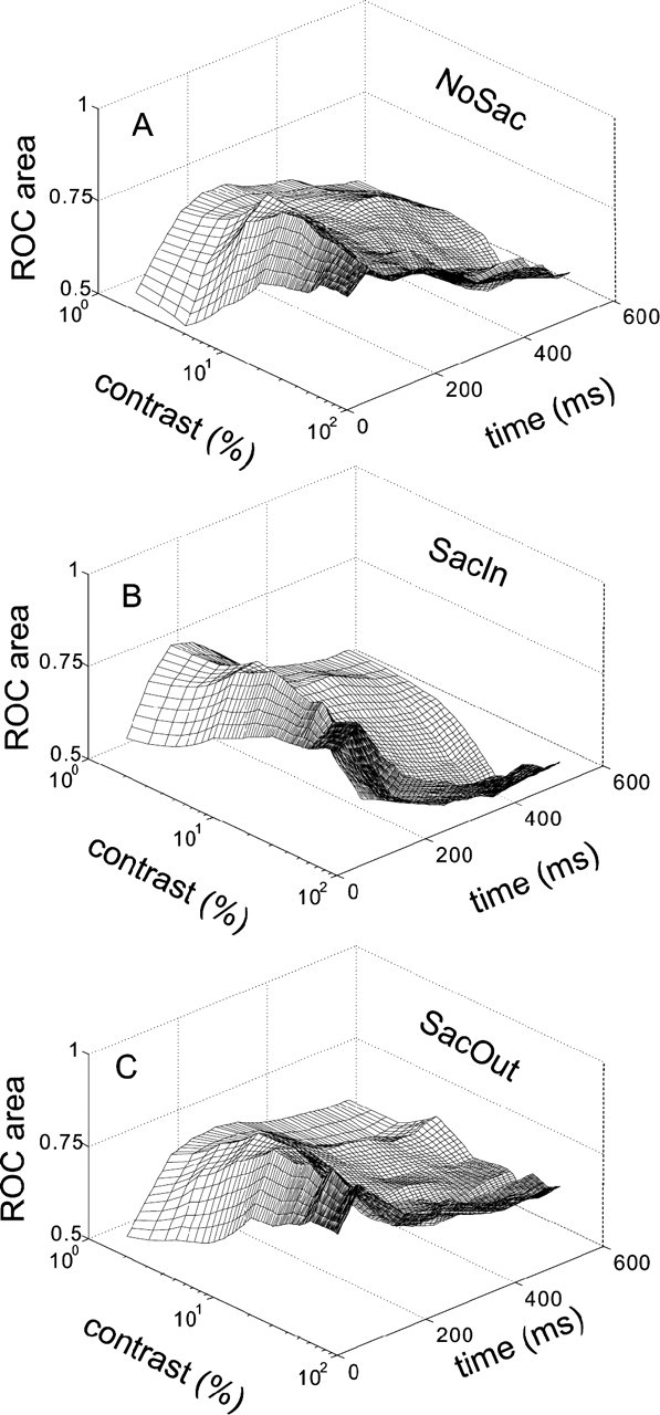
Dynamics of neuronal contrast sensitivity in SC. ROC area is plotted against contrast and time for the 79 SC neurons. A, ROC area in NoSac condition. Each line on the contrast–ROC plane is a neurometric function. ROC area was computed (see Materials and Methods) for the first 100 ms interval of neuronal discharge measured in the NoSac condition compared with the postcue neuronal baseline discharge measured in the NoSac condition. In 50 ms steps, we advanced the 100 ms analysis interval forward in time and recomputed the ROC values compared with the baseline. Then we interpolated points in the time axis every 10 ms and in the contrast axis every 1% contrast. We then plotted the result in mesh form. B, Same as in A for the SacIn condition trials. Each line on the contrast–ROC plane is a neurometric function. C, The same as in A and B but for the SacOut condition trials. For the SacIn condition, the neurometric functions are shifted to the left compared with the neurometric functions from the SacOut condition in first several time intervals.

Figure 11.

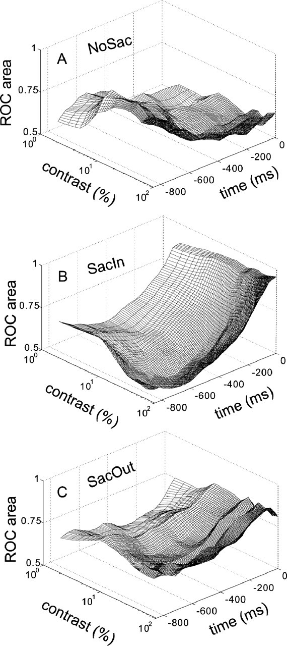
SC neuronal modulation with contrast diminishes as saccade onset approaches. The analysis and arrangement of this figure is the same as in Figure 10. For this figure, the neuronal data were aligned on the saccade onset, the analysis interval moved backward in time, and the ROC was recomputed. Note that, although the SC neurons are less modulated in contrast at the time so close to the onset of the saccade, they are still modulated by the cueing condition at this time.

What is apparent immediately from these figures is that the ability of SC neurons to detect the presence of a luminance grating within their RF changes over time. Even when monkeys remained fixating, as time evolved from the 0 to 100 ms interval to the 300 to 400 ms interval after the gratings appeared, the ROC areas across contrasts differed. Initially, ROC areas were close to 0.50 for low contrasts (Fig. 10A, bottom left curve). As time evolved, the ROC area was high even for low-contrast stimuli (Fig. 10A, top part of curve). Thus, just with time, SC neurons were better able to detect the presence of a stimulus in their RF. When a cue to make a saccade was provided, the time course of detection across stimulus contrasts seemed to evolve more quickly. The ROC area for low contrasts was higher in the SacIn condition compared with the NoSac condition (Fig. 10B, bottom curves, A, bottom curve). Furthermore, by the 100–200 ms interval, the ROC areas in the SacIn condition were ∼0.65. An ROC area of ∼0.65 occurred much later at the 200–300 ms interval in the NoSac condition. The ROC areas over time in the SacOut condition fell between those seen in the SacIn and NoSac conditions (Fig. 10C). We should point out that, although all the measurements reported here were obtained from trials presented in blocks (although the stimulus contrasts appeared randomly within blocks) and the differences between conditions were generally larger in blocked compared with interleaved conditions, they were not dependent on blocking (supplemental Fig. 2, available at www.jneurosci.org as supplemental material). This blocking phenomenon is true of some experiments performed in cortex as well (Luck et al., 1993; Reynolds et al., 2000; Williford and Maunsell, 2006).

When the same curves were drawn beginning at saccade onset and extending backward in time for 850 ms, a slightly different picture emerged (Fig. 11). The ROC areas across contrasts varied little by 850 ms before saccade onset. Nevertheless, the ROC areas measured in the SacIn condition were higher than those measured in the SacOut condition for most time intervals before the saccade (Fig. 11A,B). The ROC areas measured for the SacOut condition fell between the NoSac and SacIn conditions.

Saccade selection and preparation increase SC baseline discharge

The selection of a visual object often is associated with an increase in nondriven or baseline discharge of neurons in both the ventral and the dorsal visual cortex (Colby et al., 1996; Luck et al., 1997). We were careful throughout all analyses thus far to remove the postcue baseline activity from the stimulus-driven activity to avoid skewing the results, although this likely also minimized the differences obtained with the different cueing conditions. To compare with the results of others, we also measured specifically whether baseline changes were evident in SC neurons.

To assess the changes in baseline activity of SC neurons, we measured the discharge rate of SC neurons −200 to 0 ms from the onset of the luminance gratings but after the color cue provided information about where to look, in the three conditions (Fig. 12). Across the sample of SC neurons (n = 79), the baseline discharge rate measured in the SacIn condition compared with the baseline discharge rate measured in the NoSac condition was increased by 211.8%. The median discharge rate during baseline in the NoSac condition was 3.4 sp/s, whereas the median discharge rate during baseline in the SacIn condition was 10.6 sp/s. These differences were statistically significant (Fig. 12A) (Wilcoxon's test, p < 0.01). Among the largest, changes appeared in visual motor neurons of the SC (Fig. 12, blue triangles) (median of 11.9 sp/s SacIn; median of 6.4 sp/s NoSac). Among the smallest, changes appeared in visual tonic neurons (Fig. 12, red rightward triangles) (median of 9.2 sp/s SacIn; median of 5.9 sp/s NoSac). Across all neurons, the median discharge rate in the SacOut condition was 3.6 sp/s, and this rate was not significantly different from that measured in the NoSac condition (median of 3.4 sp/s; Wilcoxon's test, p = 0.13) (Fig. 12B). This finding indicates that the increases in baseline discharge were specific for the condition in which the upcoming saccade would be made into the RF. Thus, the changes we observed in baseline discharges of SC neurons were spatially restricted. Consistent with this conclusion, when we compared the baseline discharge of SC neurons in the SacIn and the SacOut conditions, neurons in the SacIn condition had higher discharge rates than in the SacOut condition, and these differences were statistically significant (Wilcoxon's test, p < 0.01) (Fig. 12C). Again, among the largest differences appeared for visual motor neurons (median of 11.9 sp/s SacIn; median of 4.5 sp/s SacOut) (Fig. 12, blue triangles). Figure 12D provides a composite visual representation of the data shown in Figure 12A–C. We plotted the logarithm of the ratio of baseline activities between the SacIn and NoSac conditions versus the logarithm of the ratio of baseline activities in the SacOut and NoSac conditions. Points lying in the upper right quadrant show neurons with spatially restricted increases in baseline activity.

Figure 12.

Saccade selection and preparation increases the baseline discharge of SC neurons. In A–C, each symbol indicates the mean discharge rate (spikes per second) measured −200 to 0 ms from the onset of the contrast stimuli but after the appearance of the color cue, from one neuron. The oblique line in each panel indicates unity. Symbols above the line indicate higher discharge rates in one condition versus the other. Symbols below the line indicate lower discharge rates in one condition over another. A, Baseline discharge plotted for the SacIn condition against the NoSac condition. Most points lie above the line, indicating that neurons have higher baseline activity in the SacIn condition compared with the NoSac condition (Wilcoxon's test, p < 0.01). B, Same as in A for SacOut and NoSac conditions (Wilcoxon's test, p = 0.13). C, Same as in A and B for the SacIn and SacOut conditions (Wilcoxon's test, p < 0.01). D, The ratios of baseline activity between conditions were calculated and the logarithms of the ratios plotted. The symbols above the horizontal dashed line indicate higher baseline activity for neurons in the SacIn than in the NoSac conditions. The symbols above the oblique line indicate higher baseline activity for neurons in the SacIn than in the SacOut conditions. Symbols to the right of the vertical line indicate higher baseline activity for neurons in the SacOut compared with the NoSac conditions. In all panels, circles indicate buildup neurons, upward triangles are visual motor neurons, rightward triangles are visual tonic neurons, and squares are visual phasic neurons. E, Baseline interval (−200 to 0 ms from the onset of the luminance gratings but after the appearance of the color cue) of neuronal discharge is plotted against trial number. All 79 SC neurons contributed data to this plot. Each interval was measured for each neuron for each trial. Trial number 1 is the first time the cue was presented, and error trials are included in the count.

As indicated in the preceding section, the baseline analysis provided evidence that the monkeys effectively used the color cue that indicated where to look. By exploring the time course across trials of the baseline discharge rate in the three cue conditions, we found that the increase in baseline discharge rate appeared within the first few trials (Fig. 12E). Furthermore, the baseline rate increases seen in the SacIn condition were maintained throughout the block (Fig. 12E shows 100 trials). This result confirms that the monkeys were well trained and that the cue provided useful information to the monkeys regarding the upcoming saccade. That the baseline neuronal activity was higher in the SacIn condition than in either the NoSac or SacOut conditions indicates that the baseline activity predicts the instruction cue rather than the endpoint of the eye movement. This is similar to the observation made previously for delay-period activity of SC neurons (Glimcher and Sparks, 1992).

Saccade selection and preparation decrease SC visual response latency

So far, we have shown that SC neurons have increases in the ability to detect a stimulus as well as increases in sensitivity to stimulus contrast when the stimulus will be selected as a target for a saccade. The increase is most apparent when a saccade into the RF will be made. There are also slight but significant increases in detectability and sensitivity when a saccade will be made out of the RF, indicative of a nonspatially selective signal influencing the SC. These changes are most apparent in visual motor, buildup, and visual tonic neurons but are less likely to appear in visual phasic neurons (Tables 1, 2). We also found that nonstimulus-driven or baseline activity was modulated only by a spatially restricted signal, and the change in baseline activity appeared mostly on visual motor neurons. To assess further the task influences on different SC neurons types, we explored the latency of the initial visual response of SC neurons. To define the visual latency of a neuron, we used two methods. In the first, we measured the mean and SD of the baseline neuronal activity (−200 to 0 ms from target onset but after the cue, indicating where to look). If, at a time point after the target onset, the initial visual response was higher than the mean plus 2× SD of baseline activity and lasted for at least 15 ms, this point was taken as the visual response latency. The low responding of neurons in the 2% contrast trials made this condition error prone, so we excluded this contrast condition from the analysis. Note also that the number of neurons is variable across conditions because, if we failed to detect a consistent time of the on response, we excluded the neuron from the analysis. In the second analysis, we used a method used by others in V4 (Lee et al., 2007; Sundberg et al., 2007). For this method, we measured latency as the time that neuronal discharge rate reached half of the distance between baseline activity and the peak response in the 0–200 ms time interval after the stimuli onset. The results obtained with the two methods were very similar except for two points. First, using the first method, we found decreases of the latency of the initial visual response only in buildup and visual motor neurons, but using the second method revealed that the latency of the visual tonic neurons also changed significantly. Second, the latency changes were most evident in low-contrast range using the first method, whereas using the second method, the latency changes were observed for both low- and high-contrast stimuli. Because the first method of detecting latency is more conservative, we describe only the results of the latency analysis using the first method below. The results using both methods are presented in Figure 13, A and B.

Figure 13.

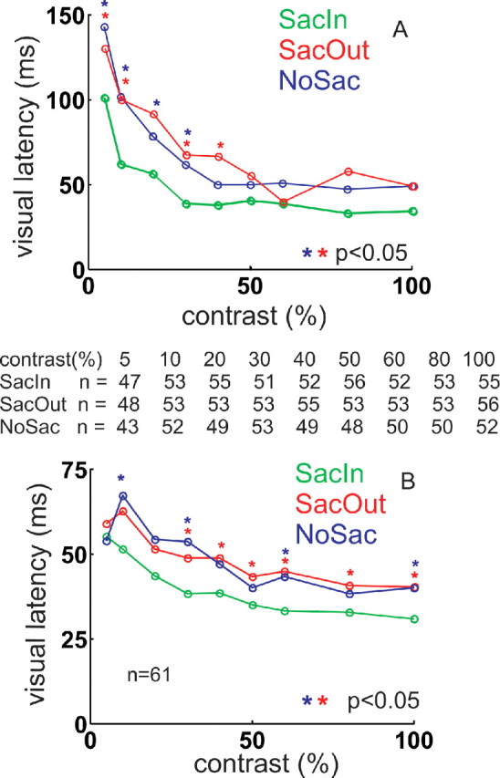
Saccade selection and preparation decreases visual response latencies of SC neurons. A, The times of the initial onset of the visual response of SC neurons are plotted against percentage contrast for each of the three task conditions. Green circles and lines are from the SacIn condition. Red circles and lines are from the SacOut condition. Blue circles and lines are from the NoSac condition. The numbers below the figure show the neuron numbers for each contrast from 5 to 100%. Red * indicates that the values in the SacOut compared with the SacIn conditions were significantly different (Mann–Whitney U test, p < 0.05, Bonferroni's corrected). Blue * indicate that the values in the SacIn and NoSac were significantly different (Mann–Whitney U test, p < 0.05, Bonferroni's corrected). B, The same as in A using the half-peak method of determining latency. Note that the data for the visual tonic and visual phasic neurons are not included in this panel for consistency with the data shown in A. Nevertheless, the visual phasic neurons had statistically significant decreases in response latency using the second method (Mann–Whitney U test, p < 0.05).

Comparing the SacIn with the NoSac conditions or the SacIn to the SacOut conditions revealed decreases of the latency of the initial visual response mainly in buildup and visual motor neurons (Mann–Whitney U modified Bonferroni's test, p < 0.05 for at least one contrast). Therefore, visual tonic and visual phasic (Mann–Whitney U test, p = NS) neurons were excluded (n = 61) (Fig. 13A). In the NoSac condition, SC neurons had long visual response latencies for low contrasts (∼150 ms) (Fig. 13A, blue circles and lines). As the contrast increased, the visual latency of SC neuronal activity gradually decreased. The latency of the initial visual response for SC neurons approached a lower asymptote at ∼50 ms (Fig. 13A, blue circles and lines).

This trend was evident for the initial visual response latency across all cueing conditions. We found, however, that the latency of the initial visual response could be modulated by the cueing conditions. In comparing the SacIn and NoSac conditions, we found that the SacIn condition was associated with reduced visual onset latencies. This was particularly evident for low contrasts (Fig. 13A, compare green and blue lines, blue *p < 0.05, Mann–Whitney U test).

We also compared the latency of the visual response of SC neurons between the SacOut and NoSac conditions to determine whether this modulation was spatially restricted like the baseline effects or whether it also had a nonspatial component like the neuronal detectability and sensitivity effects. We found that the latencies of the visual response of SC neurons in the SacOut condition were statistically indistinguishable from those measured in the NoSac condition (Fig. 13A, compare red and blue lines; Mann–Whitney U test, p = NS). Finally, to confirm the apparent spatial selectivity of the modulation of the initial response latency of SC neurons, we compared the latency measured for the SacIn condition and the SacOut condition. The visual response latency for neurons measured in the SacIn condition was significantly shorter than that measured in the SacOut condition (Fig. 13A, compare red and green lines, and red *p < 0.05, Mann–Whitney U test). Thus, the influence of the cueing condition on initial visual response latency is spatially selective.

Discussion

We present a number of new findings. First, SC neurons are responsive to luminance contrast. Whereas others found contrast responses of SC neurons of the superficial layer in anesthetized cats (Bisti and Sireteanu, 1976) and in humans using functional magnetic resonance imaging (Schneider and Kastner, 2005), as far as we are aware, this is the first documentation of contrast responses in the intermediate SC in behaving monkeys. Second, SC neurons discharged with a higher rate for the same stimulus contrast when a cue to make a saccade to a target location appeared. SC neurons with visual responses showed this enhancement: those likely within the superficial layers (Goldberg and Wurtz, 1972a; McPeek and Keller, 2002) (visual-phasic) and those likely within the intermediate layers (visual tonic, visual motor, and buildup). Third, visual tonic, visual motor, and buildup neurons showed increases in the ability to detect a stimulus and increases in sensitivity to contrast with a cue to make a saccade. Fourth, the stimulus detectability of SC neurons changed over time from the initial target onset to the time of movement onset. Finally, baseline activity of SC neurons increased and the visual on response latency decreased when the stimulus in the RF would become the saccade target compared with when the saccade out of the RF was cued or no saccade was cued. Below we compare these results with those described previously in the visual system and then in SC.

Comparison with previous studies in the visual system

The range of contrast sensitivities of visual responses in our sample of SC neurons parallels that reported for primary visual cortex (V1) neurons and magnocellular LGN neurons in anesthetized monkeys. For example, the mean C₅₀ value (also referred to as semisaturation contrast) of V1 neurons is 24.0% contrast (Albrecht and Hamilton, 1982). This is strikingly similar to what we found for visual phasic neurons (24.1%) (Fig. 3A). These neurons are likely to be in the superficial layers of SC and are likely to be those receiving input from V1 (Schiller et al., 1974; Fries, 1984; Harting et al., 1992). A direct comparison across regions showed that the median C₅₀ obtained from magnocellular LGN neurons was 11.0%, whereas the median C₅₀ from V1 was 33.0% (Sclar et al., 1990). The median C₅₀ value for the anesthetized monkey MT is 7.0% (Sclar et al., 1990), whereas that reported for awake monkey V4 is 15.0% (Williford and Maunsell, 2006). Overall, the range of C₅₀ values we found for SC is consistent with previous reports across the visual system and in visual cortex, consistent with the inputs to the SC (Fries, 1984; Harting et al., 1992).

The modulations of SC neurons with cueing conditions reported here are similar but not identical to those seen in extrastriate cortex during attention tasks. Therefore, it is useful to compare the results directly. Reynolds et al. (2000) assessed the influence of attention on luminance contrast responding and sensitivity of V4 neurons. When the orientation of a bar stimulus (test) matched the orientation of a sample bar stimulus and the location of the test stimulus and attention overlapped spatially, V4 neurons showed increases in neuronal activity compared with when attention was located outside of the RF. The increases in activity were most evident for conditions in which the stimuli had low contrasts and, combined with the ROC analysis, indicated an increase in neuronal sensitivity (but see Williford and Maunsell, 2006). The observation is similar to what we observe in SC with a notable difference. We found that increases in SC neuronal discharge rate occurred for stimuli with higher contrasts and for stimuli with low contrasts, although the increase in sensitivity was larger for low-contrast stimuli. Across V4 neurons, attention increased the absolute discharge rate of neurons by ∼24% at the best contrast (the second lowest contrast tested). Across SC neurons, a cue to select and prepare a saccade increased the discharge of neurons ∼75% at the best contrast (5%, the second lowest contrast). Across V4 neurons, the influence of attention was to increase the effective contrast of the stimulus by ∼51%. We found that a cue to select and prepare a saccade also increased the effective contrast of SC neurons by 52.3%. Thus, overall the signals indicting a cue to select a saccade influence sensory processing in much the same way as attention influences sensory processing in V4 (Reynolds et al., 2000; Reynolds and Chelazzi, 2004; Williford and Maunsell, 2006) and MT (Martinez-Trujillo and Treue, 2002) and behavior (Ling and Carrasco, 2006).

There are critical differences between V4 in the attention task and SC in the task reported here. First, no change in the latency of the visual response was observed in V4 neurons with attention, although physical changes in contrast of stimuli result in decreases in visual latency in V4 (Reynolds et al., 2000; Williford and Maunsell, 2006; Lee et al., 2007) or even lateral intraparietal area (Bisley et al., 2004), although a recent report in V4 indicates that small changes are apparent (Sundberg et al., 2007). In SC, we found robust changes in the latency of the initial visual response with a cue to make a saccade as well as with physical increases in contrast. Therefore, the cue to make a saccade influences sensory processing in the SC much like adjusting the physical contrast of the stimulus, apparently even more so than attention (Reynolds et al., 2000; Reynolds and Chelazzi, 2004; Williford and Maunsell, 2006; Sundberg et al., 2007).

A second difference between V4 and SC appears in the timing of the modulation. In most studies of attention in extrastriate cortex, the influence arises in the later part of the initial response of neurons, usually between 125 and 150 ms (Motter, 1993, 1994; McAdams and Maunsell, 1999; Reynolds et al., 2000; Hayden and Gallant, 2005), although there is some evidence for an influence as early as 75 ms (Luck et al., 1997). In the SC, we found an influence of a cue to select and prepare a saccade on the initial visual response (50–100 ms). This more closely approximates the time of modulation seen in V1 (McAdams and Reid, 2005).

A third difference between V4 in attention tasks and SC in the saccade selection task reported here is the influence of the cue on baseline activity. We found robust changes in baseline discharge rate lasting throughout the block of trials (typically >150 trials). In V4, reports of changes in baseline range from increases (1.1–4 sp/s) (Luck et al., 1997; Reynolds et al., 2000) to no statistically significant changes in baseline activity (McAdams and Maunsell, 1999). Across all SC neurons (n = 79) the median increase was 7.2 sp/s. In summary, although the differences between the phenomena in V4 and SC are sufficient to rule out the hypothesis that the effects in SC arise from V4 or vice versa, the similarities are sufficient to provide additional support for the premotor theory of attention (Sheliga et al., 1994).

Comparison with previous studies in SC

The original reports of enhancement in monkey SC described increases in the visual response of superficial layer neurons when a stimulus was used as a target for a saccade compared with when the same stimulus was ignored (Goldberg and Wurtz, 1972b; Wurtz and Mohler, 1976). What we describe here is different from the original enhancement results in two respects. First, in the original enhancement experiments, the appearance of the target was also the cue to make the saccade. What we describe here is the enhancement of neuronal discharge with a cue to select and prepare to make an eye movement. In our task, the saccade does not occur for many milliseconds after the appearance of the cue. Thus, we found that SC neurons show enhanced sensory responses with the signal to choose a saccade, whereas the original enhancement studies showed increased sensory responses during the generation of a saccade.

A second difference between the original enhancement experiments and the results reported here is that, in the original experiments, the likelihood of finding a neuron showing enhanced responses declined with depth in the SC (Goldberg and Wurtz, 1972b; Wurtz and Mohler, 1976). Furthermore, enhancement was absent from movement neurons. Our neurons defined as visual motor may be the same as those defined as “M cells” (Goldberg and Wurtz, 1972b; Wurtz and Mohler, 1976) because both neuron types are found at approximately the same depth below the SC surface. The difference in results cannot be compared directly, however, because in our task we used stimuli varying in contrast and found maximal effects within the dynamic range of the neuronal responses. In the enhancement studies, they used a single stimulus contrast that was likely high. Second, we used a visually guided, delayed-saccade task, and it was the appearance of the cue to make a saccade that resulted in the enhanced sensory responses. In the original enhancement experiments, the appearance of the target was also the cue to make the saccade. In the latter task, the visual and motor activities coalesce in time, whereas in a delay-task these activities are separate. Perhaps any visual response that may have occurred in their movement neurons was overwhelmed by the saccade-related increase, making enhancement effects difficult to discern.

A third apparent difference between our results and those of the original enhancement experiments is that we found an increase in sensory discharge and sensitivity even when monkeys received a cue to select and prepare a saccade out of the RF. The increases in discharge and sensitivity in the SacOut condition, however, were not as large as those seen in the SacIn condition. In the original experiments, enhancement was described as being spatially limited. When saccades were made out of the RF but within the same hemifield, some enhancement was reported (Wurtz and Mohler, 1976, their Fig. 4). When saccades were made out of the RF into the opposite RF, an emphasis was placed on the neurons that showed no enhancement (Wurtz and Mohler, 1976, their Fig. 2). A careful reading of their text revealed that some neurons did show enhanced responses in the out of the RF condition. The effect, however, was always smaller than that seen in the saccade into the RF condition (Wurtz and Mohler, 1976, p 748). Therefore, we conclude that this aspect of our results is compatible with that reported previously.

The results reported here demonstrate that changes in neuronal sensitivity to contrast, increases in baseline activity, and decreases in sensory response latency with cues to make saccades were most evident for buildup and visual motor neurons. Based on these results, we propose that these neurons, rather than the visual phasic, visual tonic, or saccade-related burst (not reported here), are part of the circuitry involved in identifying saccade goals. This conclusion is consistent with recent reports in a target selection task showing that buildup neurons and not burst neurons are modulated by target probability (Basso and Wurtz, 1997, 1998) and that visual motor neurons with prominent visual responses discriminate the presence of a target in the RF independent of when the saccade occurs (Horwitz and Newsome, 2001; McPeek and Keller, 2002).

A final interesting result we observed was that the modulation of neuronal sensitivity to contrast was found in movement-related neurons such as buildup and visual motor neurons, whereas the more general increase in neuronal discharge rate (enhancement of neuronal responses) was found in all four types of neurons. This suggests that the properties of inputs to as well as the local circuitry within the SC play important roles in selection. Future work exploring the cortical and corticobasal ganglia inputs to these neurons should reveal the details of the circuits underlying selection for action.

References

- Albrecht DG, Hamilton DB. Striate cortex of monkey and cat: contrast response function. J Neurophysiol. 1982;48:217–237. doi: 10.1152/jn.1982.48.1.217. [DOI] [PubMed] [Google Scholar]
- Armstrong KM, Fitzgerald JK, Moore T. Changes in visual receptive fields with microstimulation of frontal cortex. Neuron. 2006;50:791–798. doi: 10.1016/j.neuron.2006.05.010. [DOI] [PubMed] [Google Scholar]
- Basso MA, Wurtz RH. Modulation of neuronal activity by target uncertainty. Nature. 1997;389:66–69. doi: 10.1038/37975. [DOI] [PubMed] [Google Scholar]
- Basso MA, Wurtz RH. Modulation of neuronal activity in superior colliculus by changes in target probability. J Neurosci. 1998;18:7519–7534. doi: 10.1523/JNEUROSCI.18-18-07519.1998. [DOI] [PMC free article] [PubMed] [Google Scholar]
- Becker W, Jürgens R. An analysis of the saccadic system by means of double step stimuli. Vision Res. 1979;19:967–983. doi: 10.1016/0042-6989(79)90222-0. [DOI] [PubMed] [Google Scholar]
- Bell A, Meredith M, Van Opstal A, Munoz D. Stimulus intensity modifies saccadic reaction time and visual response latency in the superior colliculus. Exp Brain Res. 2006;174:53–59. doi: 10.1007/s00221-006-0420-z. [DOI] [PubMed] [Google Scholar]
- Bisley JW, Krishna BS, Goldberg ME. A rapid and precise On-response in posterior parietal cortex. J Neurosci. 2004;24:1833–1838. doi: 10.1523/JNEUROSCI.5007-03.2004. [DOI] [PMC free article] [PubMed] [Google Scholar]
- Bisti S, Sireteanu RC. Sensitivity to spatial frequency and contrast of visual cells in the cat superior colliculus. Vision Res. 1976;16:247–251. doi: 10.1016/0042-6989(76)90107-3. [DOI] [PubMed] [Google Scholar]
- Bradley A, Skottun BC, Ohzawa I, Sclar G, Freeman R. Visual orientation and spatial frequency discrimination: a comparison of single neurons and behavior. J Neurophysiol. 1987;57:755–772. doi: 10.1152/jn.1987.57.3.755. [DOI] [PubMed] [Google Scholar]
- Britten KH, Shadlen MN, Newsome WT, Movshon JA. The analysis of visual motion: a comparison of neuronal and psychophysical performance. J Neurosci. 1992;12:4745–4765. doi: 10.1523/JNEUROSCI.12-12-04745.1992. [DOI] [PMC free article] [PubMed] [Google Scholar]
- Carandini M, Heeger DJ, Movshon JA. Linearity and normalization in simple cells of the macaque primary visual cortex. J Neurosci. 1997;17:8621–8644. doi: 10.1523/JNEUROSCI.17-21-08621.1997. [DOI] [PMC free article] [PubMed] [Google Scholar]
- Carello CD, Krauzlis RJ. Manipulating intent: evidence for a causal role of the superior colliculus in target selection. Neuron. 2004;43:575–583. doi: 10.1016/j.neuron.2004.07.026. [DOI] [PubMed] [Google Scholar]
- Cavanaugh J, Wurtz RH. Subcortical modulation of attention counters change blindness. J Neurosci. 2004;24:11236–11243. doi: 10.1523/JNEUROSCI.3724-04.2004. [DOI] [PMC free article] [PubMed] [Google Scholar]
- Colby CL, Goldberg ME. Space and attention in parietal cortex. Annu Rev Neurosci. 1999;23:319–349. doi: 10.1146/annurev.neuro.22.1.319. [DOI] [PubMed] [Google Scholar]
- Colby CL, Duhamel JR, Goldberg ME. Visual, presaccadic and cognitive activation of single neurons in monkey lateral intraparietal area. J Neurophysiol. 1996;76:2841–2852. doi: 10.1152/jn.1996.76.5.2841. [DOI] [PubMed] [Google Scholar]
- Crist CF, Yamasaki DSG, Komatsu H, Wurtz RH. A grid system and a microsyringe for single cell recording. J Neurosci Methods. 1988;26:117–122. doi: 10.1016/0165-0270(88)90160-4. [DOI] [PubMed] [Google Scholar]
- Deubel H, Schneider WX. Saccade target selection and object recognition: evidence for a common attentional mechanism. Vision Res. 1996;36:1827–1837. doi: 10.1016/0042-6989(95)00294-4. [DOI] [PubMed] [Google Scholar]
- DeValois RL, DeValois KK. Spatial vision. Oxford: Oxford UP; 1990. [Google Scholar]
- di Pellegrino G, Wise SP. Visuospatial versus visuomotor activity in the premotor and prefrontal cortex of a primate. J Neurosci. 1993;13:1227–1243. doi: 10.1523/JNEUROSCI.13-03-01227.1993. [DOI] [PMC free article] [PubMed] [Google Scholar]
- Dorris MC, Munoz DP. Saccadic probability influences motor preparation signals and time to saccadic initiation. J Neurosci. 1998;18:7015–7026. doi: 10.1523/JNEUROSCI.18-17-07015.1998. [DOI] [PMC free article] [PubMed] [Google Scholar]
- Edelman JA, Keller EL. Dependence on target configuration of express saccade-related activity in the primate superior colliculus. J Neurophysiol. 1998;80:1407–1426. doi: 10.1152/jn.1998.80.3.1407. [DOI] [PubMed] [Google Scholar]
- Egeth HE, Yantis S. Visual attention: control, representation, and time course. Annu Rev Psychol. 1997;48:269–297. doi: 10.1146/annurev.psych.48.1.269. [DOI] [PubMed] [Google Scholar]
- Findlay JM, Walker R. A model of saccade generation based on parallel processing and competitive inhibition. Behav Brain Sci. 1999;22:661–721. doi: 10.1017/s0140525x99002150. [DOI] [PubMed] [Google Scholar]
- Fries W. Cortical projections to the superior colliculus in the macaque monkey: a retrograde study using horseradish peroxidase. J Comp Neurol. 1984;230:55–76. doi: 10.1002/cne.902300106. [DOI] [PubMed] [Google Scholar]
- Fuchs AF, Robinson DA. A method for measuring horizontal and vertical eye movement chronically in the monkey. J Appl Physiol. 1966;21:1068–1070. doi: 10.1152/jappl.1966.21.3.1068. [DOI] [PubMed] [Google Scholar]
- Glimcher PW, Sparks DL. Movement selection in advance of action in the superior colliculus. Nature. 1992;355:542–545. doi: 10.1038/355542a0. [DOI] [PubMed] [Google Scholar]
- Goldberg ME, Wurtz RH. Activity of superior colliculus in behaving monkey. I. Visual receptive fields of single neurons. J Neurophysiol. 1972a;35:542–559. doi: 10.1152/jn.1972.35.4.542. [DOI] [PubMed] [Google Scholar]
- Goldberg ME, Wurtz RH. Activity of superior colliculus in behaving monkeys. II. Effect of attention on neuronal responses. J Neurophysiol. 1972b;35:560–574. doi: 10.1152/jn.1972.35.4.560. [DOI] [PubMed] [Google Scholar]
- Graziano MS, Hu XT, Gross CG. Visuospatial properties of ventral premotor cortex. J Neurophysiol. 1997;77:2268–2292. doi: 10.1152/jn.1997.77.5.2268. [DOI] [PubMed] [Google Scholar]
- Harting JK, Updyke BV, Van Lieshout DP. Corticotectal projections in the cat: anterograde transport studies of twenty-five cortical areas. J Comp Neurol. 1992;324:379–414. doi: 10.1002/cne.903240308. [DOI] [PubMed] [Google Scholar]
- Hayden BY, Gallant JL. Time course of attention reveals different mechanisms for spatial and feature-based attention in area V4. Neuron. 2005;47:637–643. doi: 10.1016/j.neuron.2005.07.020. [DOI] [PubMed] [Google Scholar]
- Heuer HW, Britten KH. Contrast dependence of response normalization in area MT of the rhesus macaque. J Neurophysiol. 2002;88:3398–3408. doi: 10.1152/jn.00255.2002. [DOI] [PubMed] [Google Scholar]
- Horwitz GD, Newsome WT. Separate signals for target selection and movement specification in the superior colliculus. Science. 1999;284:1158–1161. doi: 10.1126/science.284.5417.1158. [DOI] [PubMed] [Google Scholar]
- Horwitz GD, Newsome WT. Target selection for saccadic eye movements: prelude activity in the superior colliculus during a direction-discrimination task. J Neurophysiol. 2001;86:2543–2558. doi: 10.1152/jn.2001.86.5.2543. [DOI] [PubMed] [Google Scholar]
- Kaplan E, Shapley RM. X and Y cells in the lateral geniculate nucleus of macaque monkeys. J Physiol (Lond) 1982;330:125–143. doi: 10.1113/jphysiol.1982.sp014333. [DOI] [PMC free article] [PubMed] [Google Scholar]
- Keppel G. Ed 3. Upper Saddle River, NJ: Prentice-Hall; 1991. Design and analysis: a researcher's handbook. [Google Scholar]
- Kowler E, Anderson E, Dosher B, Blaser E. The role of attention in the programming of saccades. Vision Res. 1995;35:1897–1916. doi: 10.1016/0042-6989(94)00279-u. [DOI] [PubMed] [Google Scholar]
- Lee J, Williford T, Maunsell JHR. Spatial attention and the latency of neuronal responses in macaque area V4. J Neurosci. 2007;27:9632–9637. doi: 10.1523/JNEUROSCI.2734-07.2007. [DOI] [PMC free article] [PubMed] [Google Scholar]
- Li X, Basso MA. Competitive stimulus interactions within single response fields of superior colliculus neurons. J Neurosci. 2005;25:11357–11373. doi: 10.1523/JNEUROSCI.3825-05.2005. [DOI] [PMC free article] [PubMed] [Google Scholar]
- Li X, Kim B, Basso MA. Transient pauses in delay-period activity of superior colliculus neurons. J Neurophysiol. 2006;95:2252–2264. doi: 10.1152/jn.01000.2005. [DOI] [PubMed] [Google Scholar]
- Ling S, Carrasco M. Sustained and transient covert attention enhance the signal via different contrast response functions. Vision Res. 2006;46:1210–1220. doi: 10.1016/j.visres.2005.05.008. [DOI] [PMC free article] [PubMed] [Google Scholar]
- Luck SJ, Fan S, Hillyard SA. Attention-related modulation of sensory-evoked brain activity in a visual search task. J Cogn Neurosci. 1993;5:188–195. doi: 10.1162/jocn.1993.5.2.188. [DOI] [PubMed] [Google Scholar]
- Luck SJ, Chelazzi L, Hillyard SA, Desimone R. Neural mechanisms of spatial selective attention in areas V1, V2, and V4 of macaque visual cortex. J Neurophysiol. 1997;77:24–42. doi: 10.1152/jn.1997.77.1.24. [DOI] [PubMed] [Google Scholar]
- Martinez-Trujillo JC, Treue S. Attentional modulation strength in cortical area MT depends on stimulus contrast. Neuron. 2002;35:365–370. doi: 10.1016/s0896-6273(02)00778-x. [DOI] [PubMed] [Google Scholar]
- Maunsell JHR. The brain's visual world: representation of visual targets in cerebral cortex. Science. 1995;270:764–769. doi: 10.1126/science.270.5237.764. [DOI] [PubMed] [Google Scholar]
- McAdams CJ, Maunsell JHR. Effects of attention on orientation-tuning functions of single neurons in macaque cortical area V4. J Neurosci. 1999;19:431–441. doi: 10.1523/JNEUROSCI.19-01-00431.1999. [DOI] [PMC free article] [PubMed] [Google Scholar]
- McAdams CJ, Reid RC. Attention modulates the responses of simple cells in monkey primary visual cortex. J Neurosci. 2005;25:11023–11033. doi: 10.1523/JNEUROSCI.2904-05.2005. [DOI] [PMC free article] [PubMed] [Google Scholar]
- McPeek RM, Keller EL. Saccade target selection in the superior colliculus during a visual search task. J Neurophysiol. 2002;88:2019–2034. doi: 10.1152/jn.2002.88.4.2019. [DOI] [PubMed] [Google Scholar]
- McPeek RM, Keller EL. Deficits in saccade target selection after inactivation of superior colliculus. Nat Neurosci. 2004;7:757–763. doi: 10.1038/nn1269. [DOI] [PubMed] [Google Scholar]
- Moore T, Fallah M. Control of eye movements and spatial attention. Proc Natl Acad Sci USA. 2001;98:1273–1276. doi: 10.1073/pnas.021549498. [DOI] [PMC free article] [PubMed] [Google Scholar]
- Moore T, Fallah M. Microstimulation of the frontal eye field and its effects on covert spatial attention. J Neurophysiol. 2004;91:152–162. doi: 10.1152/jn.00741.2002. [DOI] [PubMed] [Google Scholar]
- Moschovakis AK, Karabelas AB, Highstein SM. Structure-function relationships in the primate superior colliculus. I. Morphological classification of efferent neurons. J Neurophysiol. 1988;60:232–262. doi: 10.1152/jn.1988.60.1.232. [DOI] [PubMed] [Google Scholar]
- Moschovakis AK, Scudder CA, Highstein SM. The microscopic anatomy and physiology of the mammalian saccadic system. Prog Neurobiol. 1996;50:133–254. doi: 10.1016/s0301-0082(96)00034-2. [DOI] [PubMed] [Google Scholar]
- Motter BC. Focal attention produces spatially selective processing in visual cortical areas V1, V2, and V4 in the presence of competing stimuli. J Neurophysiol. 1993;70:909–919. doi: 10.1152/jn.1993.70.3.909. [DOI] [PubMed] [Google Scholar]
- Motter BC. Neural correlates of attentive selection for color or luminance in extrastriate area V4. J Neurosci. 1994;14:2178–2189. doi: 10.1523/JNEUROSCI.14-04-02178.1994. [DOI] [PMC free article] [PubMed] [Google Scholar]
- Muller JR, Philiastides MG, Newsome WT. Inaugural article: microstimulation of the superior colliculus focuses attention without moving the eyes. Proc Natl Acad Sci USA. 2005;102:524–529. doi: 10.1073/pnas.0408311101. [DOI] [PMC free article] [PubMed] [Google Scholar]
- Munoz DP, Wurtz RH. Saccade-related activity in monkey superior colliculus. I. Characteristics of burst and buildup cells. J Neurophysiol. 1995;73:2313–2333. doi: 10.1152/jn.1995.73.6.2313. [DOI] [PubMed] [Google Scholar]
- Paré M, Wurtz RH. Progression in neuronal processing for saccadic eye movements from parietal cortex area LIP to superior colliculus. J Neurophysiol. 2001;85:2545–2562. doi: 10.1152/jn.2001.85.6.2545. [DOI] [PubMed] [Google Scholar]
- Porciatti V, Alesci R, Bagnoli P. Evoked responses to sinusoidal gratings in the pigeon optic tectum. Vis Neurosci. 1989;2:137–145. doi: 10.1017/s0952523800011998. [DOI] [PubMed] [Google Scholar]
- Prevost F, Lepore F, Guillemot J-P. Spatio-temporal receptive field properties of cells in the rat superior colliculus. Brain Res. 2007;1142:80–91. doi: 10.1016/j.brainres.2007.01.041. [DOI] [PubMed] [Google Scholar]
- Reynolds JH, Chelazzi L. Attentional modulation of visual processing. Annu Rev Neurosci. 2004;27:611–647. doi: 10.1146/annurev.neuro.26.041002.131039. [DOI] [PubMed] [Google Scholar]
- Reynolds JH, Pasternak T, Desimone R. Attention increases sensitivity of V4 neurons. Neuron. 2000;26:703–714. doi: 10.1016/s0896-6273(00)81206-4. [DOI] [PubMed] [Google Scholar]
- Rizzolatti G, Riggio L, Dascola I, Umiltá C. Reorienting attention across the horizontal and vertical meridians: evidence in favor of a premotor theory of attention. Neuropsychologia. 1987;25:31–40. doi: 10.1016/0028-3932(87)90041-8. [DOI] [PubMed] [Google Scholar]
- Rodgers CK, Munoz DP, Scott SH, Pare M. Discharge properties of monkey tectoreticular neurons. J Neurophysiol. 2006;95:3502–3511. doi: 10.1152/jn.00908.2005. [DOI] [PubMed] [Google Scholar]
- Schall JD, Thompson KG. Neural selection and control of visually guided eye movements. Annu Rev Neurosci. 1999;22:241–259. doi: 10.1146/annurev.neuro.22.1.241. [DOI] [PubMed] [Google Scholar]
- Schiller PH, Koerner F. Discharge characteristics of single units in superior colliculus of the alert rhesus monkey. J Neurophysiol. 1971;34:920–936. doi: 10.1152/jn.1971.34.5.920. [DOI] [PubMed] [Google Scholar]
- Schiller PH, Stryker MP, Cynader M, Berman N. Response characteristics of single cells in the monkey superior colliculus following ablation or cooling of visual cortex. J Neurophysiol. 1974;37:181–194. doi: 10.1152/jn.1974.37.1.181. [DOI] [PubMed] [Google Scholar]
- Schneider KA, Kastner S. Visual responses of the human superior colliculus: a high-resolution functional magnetic resonance imaging study. J Neurophysiol. 2005;94:2491–2503. doi: 10.1152/jn.00288.2005. [DOI] [PubMed] [Google Scholar]
- Schneider WX, Deubel H. Oxford: Oxford UP; 2002. Selection-for-perception and selection-for-spatial-motor action are coupled by visual attention: a review of recent findings and new evidence from stimulus driven saccade control. [Google Scholar]
- Sclar G, Maunsell JHR, Lennie P. Coding of image contrast in central visual pathways of the macaque monkey. Vision Res. 1990;30:1–10. doi: 10.1016/0042-6989(90)90123-3. [DOI] [PubMed] [Google Scholar]
- Sheliga BM, Riggio L, Rizzolatti G. Orienting of attention and eye movements. Exp Brain Res. 1994;98:507–522. doi: 10.1007/BF00233988. [DOI] [PubMed] [Google Scholar]
- Sheliga BM, Riggio L, Rizzolatti G. Spatial attention and eye movements. Exp Brain Res. 1995;105:261–275. doi: 10.1007/BF00240962. [DOI] [PubMed] [Google Scholar]
- Sparks DL, Hartwich-Young R. The neurobiology of saccadic eye movements. The deep layers of the superior colliculus. Rev Oculomot Res. 1989;3:213–256. [PubMed] [Google Scholar]
- Sundberg KA, Mitchell JF, Reynolds JH. Attention-dependent reduction in response latency differs between cell classes in macaque area V4. Soc Neurosci Abstr. 2007;33:177–10. [Google Scholar]
- Ungerleider LG, Kastner S. Mechanisms of visual attention in the human cortex. Annu Rev Neurosci. 2000;23:315–341. doi: 10.1146/annurev.neuro.23.1.315. [DOI] [PubMed] [Google Scholar]
- Williford T, Maunsell JHR. Effects of spatial attention on contrast response functions in macaque area V4. J Neurophysiol. 2006;96:40–54. doi: 10.1152/jn.01207.2005. [DOI] [PubMed] [Google Scholar]
- Wolfe JM, Horowitz TS. What attributes guide the deployment of visual attention and how do they do it? Nat Rev Neurosci. 2004;5:495–501. doi: 10.1038/nrn1411. [DOI] [PubMed] [Google Scholar]
- Wurtz RH, Goldberg ME. Activity of superior colliculus in behaving monkey. III. Cells discharging before eye movements. J Neurophysiol. 1972;35:575–586. doi: 10.1152/jn.1972.35.4.575. [DOI] [PubMed] [Google Scholar]
- Wurtz RH, Mohler CW. Organization of monkey superior colliculus: enhanced visual response of superficial layer cells. J Neurophysiol. 1976;39:745–765. doi: 10.1152/jn.1976.39.4.745. [DOI] [PubMed] [Google Scholar]