How Secure Is In Vivo Synaptic Transmission at the Calyx of Held?

Abstract

The medial nucleus of the trapezoid body (MNTB) receives excitatory input from giant presynaptic terminals, the calyces of Held. The MNTB functions as a sign inverter giving inhibitory input to the lateral and medial superior olive, where its input is important in the generation of binaural sensitivity to cues for sound localization. Extracellular recordings from MNTB neurons show complex spikes consisting of a prepotential, thought to reflect synaptic activation, followed by a postsynaptic action potential. This makes the synapse ideal to study synaptic transmission in vivo because presynaptic and postsynaptic activity can be monitored with a single electrode. Recent in vivo and in vitro studies have observed isolated prepotentials in the MNTB suggesting that, under certain stimulus conditions, synaptic transmission fails. We investigated synaptic transmission at the calyx of Held in the MNTB of the adult cat and concluded that synaptic transmission was completely secure in terms of rate of transmitted spikes. However, synaptic transmission was found to be less secure in terms of timing. With increasing spike rate, the synaptic delay showed an increase of up to 100 μs, as well as a decrease in amplitude of the action potential. This variability in delay is of a surprisingly high magnitude given the hypothesized role of these binaural circuits in sound localization and given the fact that this is one of the largest synapses in the mammalian brain.

Introduction

The medial nucleus of the trapezoid body (MNTB) is a critical component of the neural circuits for sound localization in the brainstem. Each MNTB neuron receives a giant axosomatic excitatory terminal, the so-called calyx of Held, derived from a single globular bushy (GB) cell (Tolbert et al., 1982; Spirou et al., 1990; Smith et al., 1991). It acts as a sign inverter giving inhibitory input to a variety of brainstem nuclei, including the binaural nuclei of the lateral superior olive (LSO) and the medial superior olive (MSO) (Banks and Smith, 1992; Smith et al., 1998). In the LSO, this inhibitory input generates sensitivity to interaural level differences, important for the localization of high-frequency sounds (Boudreau and Tsuchitani, 1968; Tsuchitani and Boudreau, 1969). Moreover, temporally precise inhibition by MNTB also endows LSO neurons with sensitivity to interaural time differences (ITDs) of both low- and high-frequency sounds (Caspary and Finlayson, 1991; Joris and Yin, 1995; Tollin and Yin, 2005). Finally, the MNTB has also been proposed to be important for the sensitivity of MSO neurons to ITDs (Brand et al., 2002; Grothe, 2003).

Remarkably, the activity of the MNTB cell and its globular bushy input can be monitored with a single extracellular electrode. Extracellular recordings show a complex spike (see Fig. 1 A, event A) with a prepotential (A₁) generated by the calyx and a postsynaptic action potential (A₂) (Guinan et al., 1972a,b). In the cat, Guinan and Li (1990) showed that, with acoustic stimulation, A₁ is invariably followed by A₂. However, recent studies in gerbil and mouse (Kopp-Scheinpflug et al., 2003a,b) reported isolated prepotentials to acoustic stimulation (see Fig. 1 A, event B), which were interpreted as presynaptic activity failing to elicit postsynaptic spikes. In vitro evidence (Hermann et al., 2007) also shows failures of this synapse in response to electrical stimulation mimicking physiological firing patterns. These findings suggest that the MNTB is more than a simple sign inverter. In light of these two opposing views, we reassess transmission, in vivo, at this synapse.

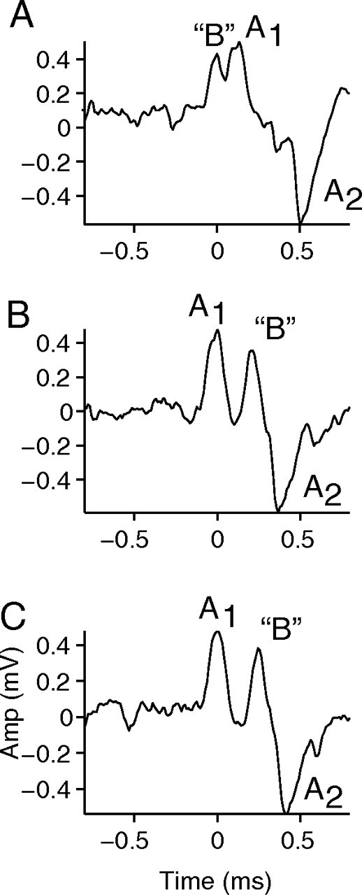
Figure 1.

One- and two-neuron hypotheses. A, Event A is a complex spike typically observed in the MNTB, composed of A₁ generated by synaptic transmission at the calyx of Held and A₂, which is the action potential of the MNTB neuron. Event B is sometimes observed in the same recordings as event A and resembles A₁ in shape. B, The one-neuron hypothesis proposes that events A and B originate from a single “complex unit” (i.e., a calyx of Held and MNTB neuron). In this case, events A₁ and B should always be separated by a time equal to or greater than the RP. C, The two-neuron hypothesis proposes that events A and B originate from two different neurons: one complex unit giving rise to event A and a second structure in the vicinity of the recording electrode giving rise to event B. Here, events A₁ and B can occur closer together than the refractory period and can overlap (“superposition”). The dashed lines indicate the trigger level use in the triggering algorithm. The long and short dead times used in the triggering algorithm are also illustrated: they are limited by the duration of events A and B, respectively.

Kopp-Scheinpflug et al. (2003a) concluded that events A and B are generated by one neuron and its synaptic input (see Fig. 1 B, “one-neuron hypothesis”). We propose that their extracellular traces reflected the potentials of two uncoupled neurons (see Fig. 1 C, “two-neuron hypothesis”), in which event B is simply a spike arising from a second neuron and the resemblance between event B and event A₁ is fortuitous. We show that, in recordings with good signal-to-noise ratios (SNRs), prepotentials are invariably followed by an action potential. In recordings in which events B are observed, a careful analysis of interspike intervals shows an absence of convincing cases of failures. Thus, with extracellular recording techniques, the GB–MNTB synapse appears secure in terms of the number of spikes transmitted: every prepotential is followed by an action potential. However, at high firing rates, the timing interval between the prepotential and spike increases with a magnitude that may be behaviorally relevant. Thus, although the synapse is secure in terms of rate, it is less secure in terms of timing.

Materials and Methods

Recording

Surgical preparation.

Adult cats with transparent eardrums were anesthetized with a mixture of acepromazine (0.2 mg/kg) and ketamine (20 mg/kg). A venous cannula allowed infusion of Ringer's solution and sodium pentobarbital at doses sufficient to maintain an areflexic state. A laryngopharyngectomy was performed and a tracheal tube was inserted. The basioccipital bone was exposed after resection of the prevertebral muscles. The pinnas were removed, and the bullas were exposed and vented with a 30-cm-long polyethylene tube (inner diameter, 0.9 mm). The animal was placed in a double-walled soundproof room (Industrial Acoustics Company). The trapezoid body (TB) was exposed by drilling a longitudinal slit as close as possible to the medial wall of the bulla and 3–5 mm rostral to the jugular foramen. A micromanipulator was used to support a five channel microdrive (TREC) with quartz/platinum–tungsten electrodes (TREC; 2–4 MΩ). The electrodes were positioned in the TB under visual control, just lateral or medial to the rootlets of the abducens nerve. The angle of penetration ranged from 15 to 20° mediolaterally relative to the midsagittal plane. After placing the electrodes in the TB, the basioccipital bone was covered with warm 3% agar.

In addition to recording from MNTB cells, we also recorded from TB axons with glass micropipettes (20–40 MΩ). We will use some of these recordings as well as similar archival recordings (Joris and Yin, 1998) to provide baseline data of single globular bushy neurons. Such neurons were identified on the basis of their responses to short characteristic frequency (CF)-tone bursts [“primary-like with notch”-shaped poststimulus time histograms (PSTHs)] and their monaural responsiveness to ipsilateral sounds (Spirou et al., 1990; Smith et al., 1991; Joris and Yin, 1998).

Hardware setup.

Dynamic speakers (Supertweeter; Radio Shack) were connected with tubing to Teflon earpieces that fit tightly in the transversely cut ear canals. The stimuli were generated digitally (PD1 System 2; Tucker-Davis Technologies) and were compensated for the acoustic transfer function measured with a probe tube near the eardrum and a 12.7 mm condenser microphone (Brüel and Kjaer). The neural signal was amplified and filtered (0.3–3 kHz). We then used two independent setups to monitor neural activity, resulting in two sets of data. In the “standard” setup, we visualized the complex units on an oscilloscope and used the event that was most easily discriminated to extract standard pulses with a window discriminator. These pulses were then time-stamped by a timer with 1 μs resolution (ET1 System 2; Tucker-Davis Technologies). Typically, the largest and best discriminable event was A₂ (for examples, see Figs. 9, 12), but occasionally it was the leading event A₁ (see Fig. 10), as has been reported previously (Guinan and Li, 1990). The setting of stimulus parameters for subsequent data collection was guided by the results displayed on-line for these standard pulses. We developed a separate recording setup to sample the neural waveform (RX6 and RX8 System 3; Tucker-Davis Technologies; 100 kHz sampling frequency) allowing us to apply off-line triggering and spike-sorting techniques (see below). To avoid sampling of the neural signal when no events were present, the waveform was not sampled continuously but only when its absolute value exceeded a manually adjusted trigger voltage. This voltage was set high enough not to be continuously exceeded by the baseline noise, but low enough to generate triggers to events A and B (Fig. 1). A 2.3 ms snippet of the neural waveform was sampled containing 0.8 ms preceding the trigger and 1.5 ms after the trigger. If the trigger level was exceeded again within these 1.5 ms, another snippet was collected. Examples of snippets are shown in Figures 4 –7, 9, and 12. For each stimulus condition [e.g., for each stimulus frequency or sound pressure level (SPL) (see below, Stimuli and unit selection)], the first 100 snippets were saved. With this procedure, all parts of the neural waveform containing values exceeding the absolute trigger voltage (either positive or negative values) were sampled, with a maximum of 100 snippets per stimulus condition.

Figure 9.

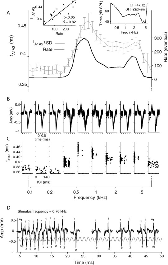
Variation in intraspike intervals. A, The thin line shows mean time (left ordinate) between peak A₁ and A₂ (t _A1A2) and its SD (error bars). The thick line shows spike rate (right ordinate). Top left inset, Linear regression analysis was used to quantify the correlation between t _A1A2 and spike rate. The solid line shows the line of best fit. Top right inset, Threshold curve showing CF and SR measured before spike sorting. B, All spikes per stimulus for a select number of stimulus frequencies. C, ISI plotted against t _A1A2 for the same stimulus frequencies. D, Spike train recorded to one repetition of the 760 Hz stimulus, with indication of events A₁ and A₂. The stimulus is superimposed.

Figure 12.

Variation in peak amplitude. A, The thin line (left ordinate) shows mean A₂ peak amplitude and its SD (error bars). The thick line (right ordinate) shows spike rate. Top left inset, Linear regression analysis was used to quantify the correlation between A₂ peak amplitude and spike rate. The solid line shows the line of best fit. Top middle inset, Mean spikes per stimulus aligned on the A₁ peak. Top right inset, Threshold curve showing CF and SR measured before spike sorting. B, Mean spike per stimulus for each stimulus frequency. C, D, A₂ peak amplitude and intraspike interval t _A1A2 plotted against ISI for each stimulus frequency. E, Spike train recorded to a segment of the 11 kHz stimulus. The decrease, at short ISIs, of the amplitude of component A₂ (but not A₂) is clearly visible.

Figure 10.

Second example of variation in intraspike intervals. A, The thin line shows mean time and SD (error bars) of t _A1A2. The thick line shows spike rate. Top right inset, Linear regression analysis to quantify the correlation between t _A1A2 and spike rate. The solid line shows the line of best fit. Top left inset, Threshold curve showing CF and SR measured before spike sorting. B, Mean spike per stimulus for a select number of stimulus frequencies.

Figure 4.

ISI analysis reveals intervals incompatible with the single-neuron hypothesis. A, After triggering and spike sorting, all events A are grouped together. B, In this recording, a second event B was also identified, which resembles event A₁ in shape. C, Spike rate against stimulus frequency for both events A and B. The inset shows the threshold curve with CF and SR, measured before spike sorting. D, E, ISI histograms for all events A₁ and B. F, Two examples in which event B precedes event A₁ by less than the RP, indicating that events A and B originate from two separate neurons. G, ISI histogram for combined events A₁ and B.

Figure 5.

Second example of the ISI analysis. For the explanation, see the corresponding panels in Figure 4.

Figure 6.

The spike-sorting algorithm misses event B when it overlaps with event A. A–C, Event “B” (manually identified) occurs just before event A₁ (A) or between events A₁ and A₂ (B, C). In all cases, the sequence of events is treated as a single complex spike.

Figure 7.

Peak aligning and cross-correlation methods. A, One stimulus group of complex spikes. The spikes are triggered on the A₁ peak, ensuring that the A₁ peaks are time aligned. The time between the A₁ and the A₂ peaks (t _A1A2) differs slightly between spikes. Therefore, the A₂ peaks are not time aligned. B, Peak-aligned spikes. All spikes are resampled so that t _A1A2 is equal to the mean t _A1A2 of the non-peak-aligned spikes. C, The solid line shows mean spike of the peak-aligned spikes. The dashed line shows mean spike of the non-peak-aligned spikes. D, E, To improve peak timing, we upsampled and cross-correlated the A₁ and A₂ peaks of the mean spike (shown in C, redrawn as shaded profiles in D) with the A₁ and A₂ peak of each upsampled, non-peak-aligned, spike.

Stimuli and unit selection.

Search stimuli were binaural tone sweeps (0.3–30 kHz; in 0.3 octave increments; duration, 250 ms; repeated every 300 ms; 60 dB SPL) delivered to both ears. A number of unit types are present in the MNTB (Guinan et al., 1972a; Guinan and Li, 1990; Spirou et al., 1990; Smith et al., 1998). In this study, we only consider recordings in which a complex spike was clearly present. Such complex spikes consist of a prepotential A₁ followed by a spike A₂. Because antidromic stimulation of MNTB neurons resulted only in component A₂ and not A₁, Guinan and Li (1990) concluded that A₁ is generated by synaptic currents on the arrival of a presynaptic spike at the calyx of Held and that A₂ is a postsynaptic action potential generated by the MNTB neuron as a direct result of A₁. When complex spikes were encountered, we determined the excitatory ear: this was always the contralateral ear. Spontaneous rate (SR) and a threshold curve were determined with the “standard” setup described above, using an automated threshold-tracking algorithm. The CF was measured from this threshold curve at the minimum threshold. Rate/level curves were collected by presenting a tone at CF with SPLs ranging from the minimum threshold to 80 dB in 5 or 10 dB steps (duration, 25 ms; repeated every 110 ms; 100 repetitions at each SPL step). Responses to frequency sweeps over a frequency range that extended beyond the limits of the threshold curve at 60 dB SPL were then collected. This wide frequency range was used because Kopp-Scheinpflug et al. (2003a) reported an increase in failures in the sidebands of the tuning curves. The responses to these stimuli are referred to as isolevel response contours. A variety of stimulus and interstimulus interval durations were used, ranging from 100 ms every 150 ms (50 repetitions) to 5 s every 6 s, at 60 dB SPL. This stimulus protocol was repeated for as many different SPLs (30–90 dB SPL) as time allowed. Recordings of the neural waveform responses to the rate/level and frequency sweep stimuli were made using our waveform recording setup.

Off-line analysis

Overview: one- or two-neuron hypothesis?

Kopp-Scheinpflug et al. (2003a) observed a mixture of events A and B in the same neural recording in the MNTB (Fig. 1). The analysis and conclusions of their study were based on the assumption that these were single-unit recordings. They argued that event B originated from the same neural element that gave rise to the prepotential, event A₁, and thus interpreted event B as a prepotential arriving at the calyx of Held but failing to elicit an action potential. We term this the “one-neuron” hypothesis (Fig. 1 B). An alternative explanation for the occurrence of a mixture of events A and B is that the recording is not derived from a single unit but reflects the potentials of two uncoupled neurons. Event B is simply the activity of a second independent neuron or fiber in the vicinity of the recording electrode that happens to resemble event A₁ in shape. We term this the “two-neuron” hypothesis (Fig. 1 C).

These hypotheses make different predictions regarding interevent intervals, which for simplicity we refer to as inter-“spike” intervals (ISIs). If events A₁ and B arise from the same globular bushy neuron, they should never occur closer together than the refractory period (RP) of a globular bushy neuron (Fig. 1 B). In that case, the ISI distribution would show a gap of ∼0.5–1 ms, as typically observed in single globular bushy neurons (Blackburn and Sachs, 1989; Spirou et al., 1990; Joris et al., 2006). However, if events A₁ and B do arise from two independent neurons, ISIs smaller than the refractory period can occur (Fig. 1 C). Note that the presence of ISIs smaller than the refractory period invalidates the one-neuron hypothesis; but if such small ISIs are not detected, neither hypothesis is falsified.

The analysis suggested is simple in principle but difficult in practice. It requires a separation of events A and B, followed by examination of the timing between sequential occurrences of both events. The key to telling which hypothesis is correct lies in the ability to detect events which occur close together (Fig. 1 B,C). However, if the events are separated by a time interval that is smaller than their individual widths, the events superimpose (Fig. 1 C). If no recording noise were present, it would be possible to decompose superpositions into the underlying events, but noise limits the ability to detect superpositions and to decompose them in routine extracellular recording. In such cases, what are really two events appears to the spike-sorting algorithm as a single event. Thus, in practice, two events must be separated by a minimum time interval to make them appear as separate events, and this minimum time interval is approximately the width (duration) of the events. The important implication is that the ISI distribution will always show a gap, even if the two-neuron hypothesis holds. This hampers the distinction between the two hypotheses. In the present study, we optimized the triggering and spike-sorting algorithm to improve the detection of ISIs smaller than the RP, critical to distinguish between the two hypotheses.

In the off-line analyses, there are several stages to label events as A or B. The first “triggering” stage detects and time-stamps events in the neural waveform and then samples snippets from the neural waveform. In the subsequent “spike-sorting” stage, wavelet analysis is used to parameterize these snippets. Superparamagnetic clustering (Blatt et al., 1996) is then used to group snippets based on their wavelet parameters. In the final stage, the different groups are inspected visually and interpreted.

Triggering.

The purpose of the triggering algorithm is to time-stamp and sample events A and B. To simplify subsequent sorting, we used a two-step “presorting” procedure in which first candidate events A were identified, and then candidate events B. We started by defining a threshold voltage level, just above the noise floor. This level was applied as both a positive and negative threshold (Fig. 1 B,C, dashed lines) so that peaks above the positive threshold or troughs below the negative threshold resulted in event times and assorted snippets. Because event A has two peaks, typically a positive component A₁ and a negative component A₂ (see Fig. 5 A) (Guinan and Li, 1990), it generates two event times and snippets, which complicates subsequent sorting. To avoid this, the triggering algorithm identified candidate complex spikes based on the polarity of peaks A₁ and A₂ and their maximum time separation (typically 0.5 ms) and passed on a single snippet per complex spike to the spike-sorting algorithm, timed on the A₁ peak. For example, in a typical recording, all event pairs consisting of a positive peak followed within 0.5 ms by a negative peak result in one snippet, timed on the positive peak A₁. For some recordings in which the duration of the complex event was somewhat longer, the maximum time separation was set to 0.6 ms. Effectively, this step to group A₁ and A₂ imposes a 0.5–0.6 ms dead time (Fig. 1 B, “long dead time”) during which no other events can be detected. This is part of the superposition problem and unavoidably results in an underdetection of the short intervals predicted by the two-neuron hypothesis (examples of such missed events are shown in Results) (see Fig. 6 B,C).

In a second step, events that have already been identified as part of candidate complex spikes are ignored, and the remaining events are timed and sampled. Again, for each event one snippet of the neural waveform is passed to the spike-sorting algorithm. To avoid multiple triggers attributable to noise, a “short” dead time of 0.2 ms is imposed so that two events cannot occur closer than the dead time (Fig. 1 C).

The dead times of the triggering algorithm set limits to the smallest detectable ISIs. Conventional triggering algorithms apply a rather long dead time [1 ms in the study by Kopp-Scheinpflug et al. (2003a)], making distinction between the one- and two-neuron hypotheses impossible. Our triggering algorithm allows us to detect (1) events B that are separated by just 0.2 ms, (2) events B that occur as close as 0.2 ms before a complex spike, and (3) events B that occur as close as 0.5 ms after an event A (timed on the A₁ peak). Thus, although it does not (because of superposition and noise) allow the capture of all events, it does allow detection of some of the event intervals that would be incompatible with the one-neuron hypothesis (intervals 2 above). However, if the one-neuron hypothesis holds, all relevant events should in principle be detectable and the dead times are not of any consequence. This is so because ISIs of globular bushy neurons always exceed 0.68 ms (see Results), so that there would never be superposition of events A and/or B if all these events were triggered by a single globular bushy neuron.

Spike sorting.

After applying our triggering algorithm to the neural recordings, we used the Wave Clus program developed by Quiroga et al. (2004) to sort the timed snippets into different groups. The Wave Clus software uses the wavelet transform to identify distinctive snippet features. A small set of wavelet coefficients is then chosen as input for the clustering algorithm. Superparamagnetic clustering (Blatt et al., 1996) on these wavelet coefficients allows semiautomatic classification of the snippets into groups consisting of similarly shaped events. Finally, we use our own software to visually check the event classification. At this stage, groups are identified as being event A, B, or neither. It is important to note that the two-step procedure in the preceding triggering algorithm (first the extraction of candidate events A and then of events B) simplifies the subsequent spike-sorting stage, because less snippets need to be sorted, but it is not essential to our analysis.

Two additional analysis steps are described in Results. One concerns measurement of the SNR of the recording. The other is a cross-correlation technique that we apply to the sampled neural signal to obtain more precise spike timing.

Results

Modeling: proof of principle

To test whether the triggering and spike-sorting method could distinguish between the one- and two-neuron hypotheses, we combined data from globular bushy axonal recordings with some simple modeling. The goal is to determine the refractory period in single globular bushy axons, and then to examine whether intervals shorter than the refractory period can be detected when responses of two neurons are mixed. To determine the refractory period of globular bushy neurons, axonal recordings were made from the TB using glass micropipettes. From these recordings, we first examined ISI distributions for rate/level functions and selected the responses at the SPL that yielded the shortest ISI. For these responses, Figure 2 shows the normalized ISI histogram (Fig. 2 A), the minimum ISI interval (Fig. 2 B), and the spike rates (Fig. 2 C), with each histogram or symbol representing one globular bushy neuron. These data show that the shortest ISI ever present in globular bushy neurons was 0.68 ms, with the vast majority of ISIs being >0.8 ms. From these data, we put the refractory period of globular bushy neurons at 0.68 ms or more (Fig. 2 A,B, dashed lines). Note that these responses include high firing rates (>500 spikes/s) (Fig. 2 C) so that our refractory period estimate is a conservative one: it is unlikely that globular bushy neurons ever generate ISIs <0.68 ms.

Figure 2.

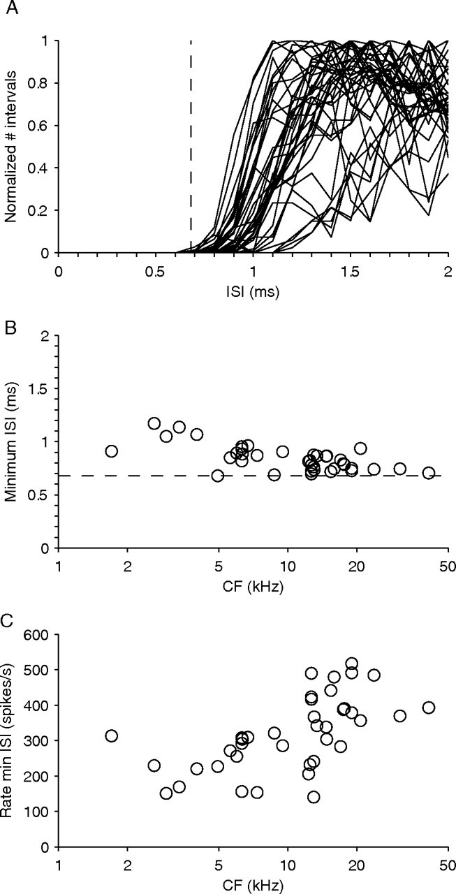
Micropipette recordings from 39 axons in the trapezoid body, identified as globular bushy by a “primary-like with notch” poststimulus time histogram to short tones at CF and monaural responsiveness to the ipsilateral ear. The data shown were obtained at the SPL generating the shortest ISI for the given neuron. A, ISI histograms normalized to the maximum number of intervals: a single histogram is shown for every globular bushy cell. B, C, Minimum interspike interval (B) and spike rate (C) as a function of CF, at the SPL generating the smallest ISI. One symbol per neuron is shown. The dashed lines in A and B indicate the smallest ISI encountered in the entire sample (0.68 ms). The bin size of the ISI histograms was 0.1 ms.

We recorded frequency sweeps, at the same SPL, from two fibers (Fig. 3 A). For the first fiber, an ISI histogram is calculated at each stimulus frequency, and all histograms are then collapsed into a single ISI histogram for all frequencies (Fig. 3 B). Here, we see that there are no intervals <0.68 ms, consistent with all spike times coming from one fiber. The same applies to the second fiber (Fig. 3 C). We then pooled the spike times from the two globular bushy axons evoked by identical stimulus presentations and computed an ISI histogram from these pooled spike times. The ISIs of the new combined group are then calculated and plotted as a histogram. For example, between 19 and 36 kHz, the isolevel response contours overlap, so the spike times for each matching stimulus frequency were combined, yielding ISIs between spikes from two different neurons. At other frequencies, the response areas do not overlap and therefore spike times did not need to be combined at these frequencies. We again collapse all ISI histograms into a single ISI histogram (Fig. 3 D). Now, intervals between 0 and 0.7 ms are apparent and indicate that the spikes times used to make this ISI histogram come from two different neurons. Note that the number of such intervals is small. This is expected because the spike times from the two fibers are independent, and because the response areas show little overlap.

Figure 3.

Modeling: proof of principle. A, Rate curves for two separately recorded GB axons with overlapping, but different, frequency tuning. B, C, ISI histograms for all spike times of GB axons 1 and 2. D, ISI histogram for merged spike times of GB axons 1 and 2. E–G, Same analysis on synthetic neural waveform, obtained by assigning event A to all spike times of GB axon 1 and event B to all spike times of GB axon 2. Triggering and spike-sorting algorithms were applied to the synthetic waveform, from which spike times were derived for events A and B. E, F, ISI histograms of all spike times of event A and B. G, ISI histogram for merged spike times of events A and B.

To test whether our spike-sorting techniques are able to reveal the small portions of critically small ISI values, we next used these combined spike times to simulate a neural recording containing spike shapes from two neurons, one generating events A and one generating events B. To do this, we superimposed an event A (Fig. 3 E, inset) onto every spike time from the first fiber, and an event B (Fig. 3 F, inset) onto every spike time from the second fiber. The simulated neural recording was then put through the same triggering algorithm and spike-sorting method used for our real data. As expected, the spike-sorting software identified two groups of spikes: events A and events B. The ISI histogram for event A (after spike sorting) is shown in Figure 3 E and is identical with that of the known spike times of the first fiber (Fig. 3 B). The ISI histogram for event B (after spike sorting) is very similar but not identical with that of the second fiber (Fig. 3, compare C, F), and the same is true for ISIs between events A and B compared with ISIs between the two fibers (Fig. 3 D,G). In the latter cases, there are less ISIs after spike sorting (Fig. 3 F,G) than in the original distributions (Fig. 3 C,D). This is attributable to the superposition problem mentioned in Materials and Methods: spikes from two separate neurons that overlap cannot be resolved as two separate events. When the smaller event B occurs at (nearly) the same time as the larger event A, the combined spike shape will most closely resemble event A (which has the larger amplitude) and will therefore be grouped with the other events A. Thus, Figure 3 E is identical to Figure 3 B, whereas Figure 3 F has fewer events than Figure 3 C. Most importantly, the superposition problem hampers the detection of small ISIs, which are critical to distinguish one-neuron from two-neuron recordings: ISIs <0.2 ms present in the combined ISI before spike sorting (Fig. 3 D) are missing in the combined ISI after spike sorting (Fig. 3 G). However, the spike-sorting method can still detect intervals that are >0.2 ms but smaller than the refractory period. The presence of such intervals indicates that more than one neuron contributes to the recording.

MNTB recordings: security in rate

Extracellular recordings that contained a complex spike (event A) were made from 49 complex units in the MNTBs of eight cats. We use the term “complex unit” because the identity of the underlying cellular substrate is unclear and is actually the subject of our study: according to the one-neuron hypothesis, it includes a calyx of Held and its postsynaptic MNTB neuron, whereas according to the two-neuron hypothesis, it includes an additional axon or calyx plus MNTB neuron (Fig. 1). The CFs measured on the threshold curves for these complex units ranged from 165 to 32,000 Hz (mean CF, 9000 Hz) and the SRs from 0 to 66.8 spikes/s (mean SR, 17.4 spikes/s). The PSTH classification of the complex units was as follows: 7 primary-like, 23 primary-like with notch, and 5 phase locked. Classification data were not available for the remaining 14 complex units. It should be cautioned that CF, SR, and PSTH classification are based on the data obtained with the “standard” recording configuration, before spike sorting (i.e., based on the event in the complex unit that was most easily discriminable) (see Materials and Methods). These data are not further used in Results, except to illustrate tuning curves in Figures 4, 5, 9, 10, and 12.

From the 49 complex units, we made a total of 186 recordings. The term “recording” refers to the sampled neural response to one set of stimulus conditions: either the frequency sweep stimuli at a given SPL or the rate/level stimuli at CF. In 18 of the 49 cases (37%), events B were never observed and the recording consisted entirely of events A. In the remaining 31 cases, we observed events B in addition to events A. For a given complex unit, events B were not necessarily present in all recordings. For example, event B could be present in a recording at high SPL but not at lower SPLs. Overall, a mixture of events A and B was observed in 77 of 186 recordings (41%).

Interspike interval analysis

Figure 4 shows a typical recording from a complex unit in the MNTB. The CF determined from the threshold curve for this unit was 1281 Hz (Fig. 4 C, inset). The range of the frequency sweep was chosen to be 300–3000 Hz (0.1 octave steps, at 60 dB SPL) to adequately cover the response limits of the threshold curve. After triggering and spike sorting, we identified two spike shapes in this recording: event A (Fig. 4 A) and event B (Fig. 4 B). Event A consists of a positive prepotential (A₁), followed ∼0.4 ms later by a biphasic action potential A₂. A positive A₁ component was consistently found in all complex units, but A₂ could be negative, positive, or biphasic. Event B resembles the prepotential of the complex spike (A₁) in shape and could be interpreted as an isolated prepotential. Event B is followed by a small “negativity” ∼0.4 ms after the main spike. Kopp-Scheinpflug et al. (2003a) also observed these small negativities after the events they classified as isolated prepotentials and suggested that these were extracellular recorded EPSPs that fail to trigger spikes.

After spike sorting, we plotted the rate of each type of event against stimulus frequency (Fig. 4 C). Note that, in this (and subsequent) figure(s), the rate for each event is calculated by dividing the number of events by the length of time it took to collect them. Because this length of time includes alternating periods of stimulation and of silence, this rate is typically lower than the spike rate traditionally reported (e.g., in Fig. 3), which takes into account only spikes that are evoked during the stimulus. In Figure 4 C, the two events show different but overlapping isolevel contours: event A has a maximum spike rate at 568 Hz and event B has its maximum spike rate at 1100 Hz. The ISI histogram of event A₁ is shown in Figure 4 D, collapsed across all stimulus frequencies. The ISI histogram of event A₂ (data not shown) would be almost identical because in this group of spikes each A₁ peak is followed by an A₂ peak (the reason the ISI histograms of A₁ and A₂ are not necessarily identical is attributable to a variable delay between A₁ and A₂ as explained in Results below, Fig. 9, and further). The ISI histograms of events A and B (Fig. 4 D,E) show no intervals less than ∼1 ms. Figure 4 G shows the combined ISI histogram for all spike times from events A and B: it shows shorter intervals than in Figure 4, D and E. Two examples are shown in Figure 4 F. Here, we clearly see that an event A₁ occurs ∼0.25 ms after an event B. This is less than the refractory period of globular bushy neurons (Fig. 2), indicating that event A₁ and B cannot originate from a single globular bushy neuron, so that event B cannot be regarded as a “failing prepotential.” Now, knowing that events A and B originate from different neurons, we can measure the best frequency (BF) for each neuron, in which BF is defined as the stimulus frequency eliciting the maximum response at a given SPL. The neuron generating event A has a BF of 568 Hz, whereas the neuron generating event B has a BF of 1100 Hz. The small negativity after event B, which was interpreted by Kopp-Scheinpflug et al. (2003a) as an EPSP failing to trigger an action potential, can now be interpreted in a different way. Event B simply reflects the activity of a second, independent, GB–MNTB synapse with a higher BF. Event B is the prepotential and the small negativity after event B is the action potential. The fact that the action potential from event B is smaller than that of event A may be because the electrode was further away from the MNTB cell body generating the event B action potential.

Figure 5 shows another example of a recording from a complex unit in the MNTB. Here, the CF was 10,530 Hz (Fig. 5 C, inset) and the range of the frequency sweep was set to 4.9–13 kHz, (0.1 octave steps, at 50 dB SPL) to cover the response limits of the threshold curve. In this recording, the spike sorter identified two different spike shapes, events A and B shown in Figure 5, A and B, respectively. Again, event B resembles event A₁ and the two events show different but overlapping isolevel contours (Fig. 5 C). The spike rate of event B is much lower than that of event A so we show spike rate on a log axis. The ISI histogram of events A shows no intervals less than ∼0.75 ms (Fig. 5 D). The ISI histogram for event B (Fig. 5 E) is very sparsely populated because there were only 70 events B in the entire recording. However, the combined ISI histogram in Figure 5 G shows a number of intervals smaller than the refractory period. Two specific examples are shown in Figure 5 F. This means that event B is not an isolated prepotential originating from the same neuron as event A₁ but is simply the activity of a second neuron in the vicinity of the recording electrode. Note that, according to the “one-neuron” interpretation, recordings as in Figures 4 C and 5 C would be interpreted as evidence for sideband inhibition, causing sharper frequency selectivity by causing “failures” in the transmission of globular bushy input to MNTB output. In the two-neuron hypothesis, Figures 4 C and 5 C would simply indicate a difference in tuning between two independent cells.

As mentioned previously, a critical problem with spike-sorting methods is the inability to detect overlapping events in extracellular recordings with typical signal-to-noise ratios. Figure 6 shows three examples in which event A and B seemingly occurred at almost the same time and in which their spike waveforms superimpose (same recordings as in Fig. 5). The spike sorter classified these waveforms as events A and did not detect separate events B. For the purposes of this figure, we manually make a tentative assignment of events “B.” In Figure 6 A, an event B seems to occur just before event A₁. In Figure 6, B and C, an event B seems interposed between event A₁ and A₂. These manual assignments are necessarily tentative, but further illustrate the point that the features that most critically differentiate the one- versus two-neuron hypotheses at least partially escape detection by spike sorting. Thus, although Figures 4 and 5 show intervals incompatible with the one-neuron hypothesis, observations as in Figure 6 suggest that there are even more intervals less than the RP than detectable by spike-sorting methods. The overlapping events cast additional doubt on the interpretation that events B are isolated prepotentials followed by an extracellularly recorded EPSP. In the cases illustrated, they are likely spikes generated by another neuron in the vicinity of the recording electrode.

Of the 31 complex units that showed a mixture of events A and B, the combined ISI histograms showed intervals <0.5 ms in 27 cases, consistent with event B originating from a different neuron than event A₁. Thus, the recordings from these 27 complex units were in fact multiunit recordings. Therefore, event B could not be classified as an isolated prepotential originating from the same neuron as event A₁. For the remaining four complex units in which the combined ISI did not show intervals <0.5 ms, we cannot rule out the possibility that events A₁ and B originated from the same neuron. For three of these complex units, the percentage of events B observed was very low (<1.1%), and observed in only one recording (i.e., one frequency sweep). Whether these latter recordings were in fact multiunit recordings is difficult to test with the ISI analysis because, given the small numbers of events B, the likelihood of it occurring closer to event A₁ than the RP is extremely small. There was only one complex unit in which a large percentage of events B was observed (8%), and no ISIs <0.5 ms were present. This unit was only held for a short time so that only one recording with sampled data was available. Thus, in our entire database, there was only one recording in which a significant number of events A₁ and B was observed and in which the combined ISI histogram was not inconsistent with the one-neuron hypothesis (but not with the two-neuron hypothesis either). In conclusion, there is no clear evidence in favor of the one-neuron hypothesis in our data.

Signal-to-noise ratio

The ISI analysis shows that, in the large majority of cases in which both events A and B were observed, these events originated from different neurons (27 of 31). Because the isolation of spikes from single neurons strongly depends on spike amplitude relative to background noise, we looked for a relationship between the SNR of the recording and incidence of events B. We quantified SNR as follows:

where Amp_signal is the root mean square (RMS) amplitude of the signal, in this case event A, and Amp_noise is the RMS amplitude of the noise. To measure the Amp_signal, we needed to measure the RMS of the mean of all occurrences of event A. However, because event A consists of at least two peaks (A₁ and A₂), and because the timing between the maxima of these peaks (t _A1A2) (Fig. 7 A) can vary (see below, Fig. 9), simply taking the mean would lead to a smearing out of the A₂ peak (Fig. 7 C, dashed line) and an underestimation of Amp_signal. Therefore, we used a peak aligning method to calculate the mean spike. For every recording, we first calculated the mean t _A1A2 and then resampled (time warped) each individual complex spike so that its t _A1A2 was exactly equal to the mean t _A1A2 (Fig. 7 B). We then calculated the mean spike of the peak aligned spikes (Fig. 7 C, solid line) and the RMS of this mean spike gave Amp_signal. To measure Amp_noise, we calculated the RMS of a section of the recording (between 1 and 15 s) in which no spikes were present. In Figure 8, we plot SNR against the percentage of events B in the recording. The percentage of events B was calculated as the number of events B divided by the number of events A plus the number of events B (total number of events). It is clear from Figure 8 that for SNRs >20 we do not observe events B in MNTB recordings (n = 32). Eight complex units had an average SNR (averaged across recordings) >20, and for these eight complex units no occurrences of event B were ever observed. This means that in the recordings that are considered to be the “cleanest,” we do not observe any occurrences of event B. Combined with the ISI analysis, this is additional evidence that events that appear to be “failing prepotentials” are in fact only observed in recordings contaminated with activity from other neurons.

Figure 8.

Event B was not encountered in recordings with high SNR. SNR is plotted against the percentage of events B for each recording (176 recordings). The percentage of events B is calculated as the number of events B divided by the number of events A plus the number of events B. Recordings in which the combined ISI analysis showed that events A₁ and B occurred closer together than the refractory period are shown as crosses; the others as circles. The dashed line is at an SNR of 20.

Qualitative observations

In addition to the ISI and SNR analyses, some qualitative observations suggest that events B were signals from neighboring neurons rather than true failures of spike transmission. In many cases, events B drifted “in and out” of the recording without any apparent relationship to the stimulus parameters. For example, in sequential runs of frequency sweeps in which SPL was pseudorandomly varied, events B could appear in a number of sequential datasets and disappear again. Small events that were similar to events B but with negative polarity were also frequently observed (in or 65 of 186 recordings from 29 of the 49 complex units). Such events would obviously never be taken for “failing prepotentials,” although they did not differ from events B except in their polarity.

MNTB recordings: postsynaptic time and amplitude

Complex spike: intraspike intervals

In some of the recordings with good SNRs, we noticed that the time between the A₁ and the A₂ peak (t _A1A2 or intraspike interval) increased with rate. The time stamps provided by the spike-sorting software are simply determined by the value of a single sample [i.e., the maxima of the A₁ and A₂ peaks (or minima in the case of some negative A₂ peaks)] which makes them sensitive to noise (Fig. 7 E shows an example). To allow us to determine the timing of the A₁ and A₂ peaks more robustly and accurately (and thus measure t _A1A2 more accurately), we developed a method that uses the following upsampling and cross-correlation technique. First, a recording was passed through the triggering algorithm and spike-sorting method described above. Then the group of events A was separated into smaller “stimulus” groups of spikes according to the stimulus frequency at which the spike was recorded (Fig. 9 B). For each stimulus group of spikes, we used the peak aligning method described above to calculate a mean complex spike (i.e., resampled each individual spike so that its t _A1A2 was exactly equal to the mean t _A1A2 of the stimulus group and then calculated the mean of these peak aligned spikes) (Fig. 7 A–C). We now went back to the original non-peak-aligned stimulus group of spikes and upsampled these by a factor of 10. The mean spike was also upsampled by a factor of 10. A small section around the A₁ peak of the mean spike, with a width equal to the full-width at half-maximum of the A₁ spike, was clipped out (Fig. 7 D,E, thick line). This A₁ clip was then cross-correlated with each individual A₁ spike, to find the temporal position of maximal correlation. The peak of the A₁ clip at that temporal position was then taken as the new time for the A₁ peak of that individual spike (Fig. 7 E). The same process was then repeated for the A₂ peak. The improvement in timing accuracy was considerable: for some recordings, this upsampling and cross-correlation technique led to a reduction of more than one-half in the SD of t _A1A2 within one stimulus group of spikes.

Figure 9 A shows an example of how t _A1A2 changes with spike rate for a neuron with CF of 4 kHz (Fig. 9 A, top right, tuning curve). This neuron shows strong phase locking in its low-frequency tail and has a BF of 760 Hz, markedly different from its CF. The stimulus here was a downward frequency sweep from 7000 to 100 Hz, in 0.2 octave steps, at 70 dB SPL. At low frequencies (100–400 Hz), the spike rate (Fig. 9 A, right ordinate, thick line) is low and t _A1A2 remains relatively constant at ∼0.38 ms (thin line with error bars showing ± SD, left ordinate). As the spike rate increases (400–700 Hz), t _A1A2 also increases to ∼0.46 ms. At still higher frequencies, the spike rate decreases except for a small secondary peak around the CF. A decrease and secondary peak are also clearly visible in the t _A1A2 plot. The inset in the top left of Figure 9 A plots t _A1A2 against spike rate for every stimulus frequency shown in Figure 9 A. Using linear regression, a significant positive correlation between spike rate and t _A1A2 was found for this recording (p < 0.05; r ² = 0.82). The solid line shows the line of best fit and has a slope of 0.3 μs · spikes⁻¹ · s⁻¹; equivalent to an increase in t _A1A2 of 30 μs for an increase in spike rate of 100 spikes/s. Figure 9 B shows a number of the stimulus spike groups positioned around the frequency at which they were collected (SNR, 31), and Figure 9 C plots their ISI against t _A1A2 (for reasons of space, only the groups at every third frequency are shown). Each dot in Figure 9 C represents the t _A1A2 of one complex event and the ISI with the preceding complex event. As the intervals between spikes decrease (or spike rate increases), we see that t _A1A2 also increases. At a stimulus frequency of 0.1 kHz, most t _A1A2 are ∼0.38 ms, but at 760 Hz the smallest t _A1A2 (∼0.42 ms) is larger than any recorded at lower stimulus frequencies. Finally, as has been reported previously for globular bushy and MNTB neurons (Joris et al., 1994a; Smith et al., 1998; Louage et al., 2005), phase-locking to low frequencies was exceptional. Figure 9 D shows a continuous spike train recorded to the first 50 ms of a 100 ms, 760 Hz stimulus, which was the frequency generating the highest response rate. The waveform of the stimulus is superimposed, and the occurrence of components A₁ and A₂ is indicated. Phase-locking is excellent over the entire stimulus duration (vector strength of 0.91, measured from A₂ over the 100 ms stimulus window), and the complex spike entrains to the stimulus over the first 20 ms of the stimulus. Even when entraining at this high discharge rate, every prepotential is followed by an action potential.

It is notable that the response rate over the first 20 ms in Figure 9 D is among the highest reported for globular bushy or MNTB neurons in response to acoustic stimulation. Entrained firing at rates >500 spikes/s has been reported previously for globular bushy neurons in response to short low-frequency tones (Joris et al., 1994a,b). Figure 9 D illustrates that such responses can be observed in the MNTB as well, without failures. Guinan and Li (1990) did observe failures in MNTB neurons in response to electrical shock trains delivered to globular bushy axons at rates ≥500 Hz, but these stimuli were several hundred milliseconds in duration. The present data show that, at firing rates that globular bushy neurons can sustain in response to acoustic stimulation, the MNTB neuron can respond without failures.

Figure 10 A shows a recording from a different complex unit with a lower SNR (SNR, 9.8), shown in the same format as Figure 9 A. The CF of the neuron measured from the threshold curve was 8706 Hz (Fig. 10 A, top left, inset). The stimulus was a downward frequency sweep from 14,000 to 4000 Hz, in 0.2 octave steps, at 60 dB SPL. A clear increase in t _A1A2 is seen with increasing spike rate. The inset in Figure 10 A shows a plot of rate against t _A1A2 and the solid line shows the line of best fit using linear regression (p < 0.05; r ² = 0.81). Again, there is a significant positive correlation between rate and t _A1A2. The line of best fit has a slope of 0.5 μs · spikes⁻¹ · s⁻¹, equivalent to an increase in t _A1A2 of 50 μs per 100 spike/s increase in spike rate. Figure 10 B shows the mean peak-aligned spike at a number of stimulus frequencies.

Linear regression analysis was used to quantify the relationship between t _A1A2 and rate for all recordings. Figure 11 shows the slope of the line of best fit against SNR. Ninety-four percent of the recordings from complex units (175 of 186 recordings) show a positive slope (i.e., an increase in t _A1A2 with increasing spike rate). This correlation was significant (p < 0.05; r ² > 0.25) in 76% of recordings (141 of 186 recordings). Considering only recordings with SNR >20 (vertical dashed line), 100% of the recordings (26 of 26 recordings) showed an increase in t _A1A2 with increasing spike rate, which was significant in all recordings except two.

Figure 11.

At the population level, intraspike interval is positively correlated with spike rate. Linear regression was used to determine the correlation between spike rate and t _A1A2 for each recording. The slope of this relationship is plotted against SNR. Each point represents the correlation analysis for one recording, across all stimulus conditions. Significant correlations (p > 0.05; r ² > 0.25) are shown with a cross, and others are shown with a circle.

Complex spike: peak amplitude

In recordings with good SNRs, we observed not only an increase in the t _A1A2 interval but also a decrease in the amplitude of the A₂ peak with spike rate. Figure 12 shows an example for a recording with excellent SNR (=561). The CF measured on the threshold curve was 11.3 kHz (Fig. 12 A, top right inset) and the downward frequency sweep was from 14 to 7 kHz, in 0.1 octave steps, at 70 dB SPL. Figure 12 B shows the peak-aligned mean spike recorded at each stimulus frequency. It is clear from the mean spikes that the amplitude of the A₂ peak (A_2-peak) decreases with increasing spike rate. The spike rate is shown as the thick line in Figure 12 A (right ordinate). The thin line shows the mean A_2-peak at each stimulus frequency ± SD (left ordinate). A_2-peak is maximally depressed at ∼11 kHz, at which spike rate is also maximal. There was a negative and significant (p < 0.05; r ² = 0.78) correlation between A_2-peak and spike rate (Fig. 12 A, top right inset; line shows the line of best fit). Importantly, the amplitude of the prepotential, A_1-peak, was not affected by spike rate. This is most easily seen in Figure 12 A, middle inset, which shows the averaged spikes of Figure 12 B on top of each other, aligned on event A₁. Clearly, A₁ is more invariant in its shape and amplitude than A₂. Figure 12 C plots A_2-peak against ISI for each stimulus frequency. Each dot shows A_2-peak for a complex event, against the ISI with the preceding complex event. As the intervals between spikes decrease (and the spike rate increases), the A_2-peak also decreases. At a stimulus frequency of 7 kHz, most A_2-peak are ∼4.6 mV, but at 11 kHz, the largest A_2-peak (∼3.5 mV) is smaller than any recorded at low stimulus frequencies. An opposite pattern is observed for t _A1A2 (Fig. 12 D). Graphing of A_2-peak as a function of t _A1A2 for all events A also shows a significant inverse correlation (r ² = 0.66; p < 0.05). Note that both metrics (A_2-peak and t _A1A2) return to their “resting” values at the edges of the frequency sweep, ruling out the possibility that these effects are attributable to a time-dependent recording artifact (such as electrode drift). Figure 12 E shows a 35 ms fragment of the spike train recorded to the 100 ms, 11 kHz stimulus. At this high spike rate, the A_2-peak is reduced, especially when the ISIs are small, but every prepotential is still followed by an action potential.

Linear regression analysis was used to quantify the relationship between A_2-peak and spike rate for all recordings. Because A_2-peak was negative in some recordings and positive in other recordings, we used the absolute A₂ peak amplitude. Figure 13 shows the slope from the line of best fit against SNR. The slopes are negative in recordings with a SNR >20 (dashed vertical line) [i.e., the amplitude of the A₂ peak decreased with spike rate (32 recordings)]. For these recordings, the negative correlation was significant (p < 0.05; r ² > 0.25) in 72% of the recordings (23 of 32 recordings). At SNRs <20, the amplitude of the A₂ peak shows no clear relation to spike rate. Interestingly, using the same analysis, we could not detect a relationship between A₁ peak amplitude and spike rate in any of the recordings (data not shown).

Figure 13.

At the population level, A₂ peak amplitude is negatively correlated with spike rate. Linear regression was to determine the correlation between spike rate and absolute A_2-peak for each recording. The slope of this relationship is plotted against recording SNR. Each point represents the correlation analysis for one recording, across all stimulus conditions. Significant correlations (p > 0.05; r ² > 0.25) are shown with a cross, and others are shown with a circle.

A possible basis for the increased t _A1A2 and decreased A_2-peak is postsynaptic depression of the EPSP (Taschenberger and von Gersdorff, 2000; Klug and Trussell, 2006). It is interesting to observe that these changes are also accompanied by an increased jitter in t _A1A2 (see larger spread of dots in Figs. 9 C, 12 D at stimulus frequencies causing high firing rates, and larger error bars for t _A1A2 in Figs. 9 A, 10 A).

Discussion

Several considerations prompted us to reevaluate in vivo synaptic transmission in the MNTB. First, the calyx of Held is one of the largest and therefore one of the best studied presynaptic terminals in the mammalian CNS. It presumably sets an upper bound on security of transmission in the CNS: if this synapse is not secure in its transmission of spikes, it is unlikely that other synapses are. Second, an explanation is needed for the discrepancy between the study by Kopp-Scheinpflug et al. (2003a), who report median failures rates of 52 and 45% for spontaneous and CF-driven activity, and previous reports that emphasized the fidelity of transmission and the similarity in response properties between globular bushy and MNTB neurons (Guinan and Li, 1990; Smith et al., 1991; Tsuchitani, 1997; Joris and Yin, 1998). In particular, Guinan and Li (1990) showed that, with acoustic stimulation, every prepotential A₁ is followed by an action potential A₂ so that the MNTB functions as a simple and reliable sign inverter. Only under electrical stimulation at high rates (≥500 Hz) did they observe failures of synaptic transmission, resulting in prepotentials not followed by action potentials.

A convincing proof of failures requires simultaneous recording of the presynaptic and postsynaptic structure. As pointed out by Kopp-Scheinpflug et al. (2003a), extracellular recording provides this opportunity because the prepotential is thought to reflect presynaptic activity. However, to distinguish between failing prepotentials (which are typically smaller in amplitude than spikes) and spikes from neighboring neurons or fibers, picked up by the same electrode, it is critical to examine ISIs. We point out that the most critical ISIs are exactly the ones that are most difficult to detect, because superpositions are problematic to detect and to decompose in typical extracellular recordings. Recordings with patch-clamp or sharp electrodes have better SNR but have low yield and, more importantly, carry a higher risk of abnormal physiology induced by physical contact with the structures studied. Optical recording methods are likely to circumvent these problems in the near future.

One- or two-neuron hypothesis?

The strongest evidence in our data against the presence of failures is the complete absence of events B (“failing prepotentials”) in the recordings with the highest SNR (average SNR >20 for eight complex units, in 32 recordings). One of the criteria that Kopp-Scheinpflug et al. (2003a) used for single-unit recording was a SNR >2. We found that a SNR of >20 was necessary to be absolutely sure of single-unit recording (Fig. 8). However, because of methodological differences (in species, electrode type, SNR definition), these numbers are probably not directly comparable. In the recordings with higher SNRs, the electrode is probably closer to the complex unit and the likelihood of recording spikes from a second unit is greatly diminished.

In 31 of 49 cases, both events A and B were observed, at least some of the time. In none of these cases was the average SNR (averaged across recordings) >20. Analysis of the ISIs of events A showed that all occurrences of event A respected the RP (i.e., they did not occur closer together than 0.5 ms). This is not surprising given that overlapping events could not be detected, limiting the resolution to the duration of the event, which was ∼0.5 ms for event A. However, the ISIs of events B also respect the refractory period. For these events, the resolution is ∼0.2 ms: the presence of a refractory period therefore suggests that events B originated from one neuron. Most importantly, when we combined the spikes times of all events A and B from one recording and calculated a combined ISI we found that there were ISIs smaller than the refractory period in 27 of the 31 cases. In these 27 cases, not all occurrences of events A₁ and B could have originated from a single calyx. Thus, the majority of recordings in which both events A and B were present (27 of 31) were in fact contaminated by events from another neuron(s), either another MNTB neuron or a globular bushy axon.

In the four cases in which we observed events A and B but no ISIs smaller than the RP, we cannot completely rule out the possibility that events A and B came from one complex unit (the one-neuron hypothesis) (i.e., that events B represented failures). Neither can we rule out the possibility that events A and B arose from two separate units (the two-neuron hypothesis). In none of these four cases was the hypothesis of failures the most plausible one. In three cases, the number of events B was extremely low (<1.1%), so that chances for ISIs less than the refractory period were very low, and the events B occurred in only one recording. In the remaining one case, the complex spike was quickly lost so that only one recording was obtained.

One may argue that, even if the recordings with events A and B contain multiunit events, this does not exclude the possibility that some of the events B are prepotentials that fail to elicit an action potential. These failing prepotentials would resemble event B (the spike from the second neuron) and so be misclassified by the spike-sorting algorithm into this group. However, in that scenario, events B should not respect the RP, which they always did.

As pointed out in Materials and Methods, we could not detect events B occurring during a complex spike. Is it possible that we missed failures occurring within complex spikes? This is again very unlikely for the simple reason that auditory responses of globular bushy neurons, recorded in the same preparation, did not show ISIs <0.68 ms. Thus, even with the quickest successive calyceal firings, an event B would never fall within the A₁–A₂ complex. Therefore, under the one-neuron hypothesis, all events A and B should be detectable with our methods, even at the shortest ISIs. The only exception we can think of is when an MNTB neuron would be innervated by more than one calyx of Held. Exceptional innervation by multiple large inputs has been surmised based on in vitro data of the mouse MNTB (Bergsman et al., 2004). Globular bushy neurons terminating in two calyces have been described anatomically (Spirou et al., 1990; Smith et al., 1991), but not ending on the same MNTB neuron. An MNTB neuron innervated by two independent globular bushy calyces would presumably show a large number of events B “buried” in the complex spike and thereby escape detection by our methods. To our knowledge, there is currently no anatomical or physiological evidence pointing to multiple MNTB calyces in the adult cat. All the evidence, taken as a whole, convinces us that with in vivo acoustic stimulation the GB–MNTB synapse is perfectly secure in terms of rate.

Our reasoning is strongly based on our own and published data in the pentobarbital-anesthetized cat, which is the species for which by far the most detailed morphological and physiological in vivo information on globular bushy and MNTB neurons is available. Kopp-Scheinpflug et al. (2003a) recorded from the gerbil MNTB using ketamine as an anesthetic. Although it is clear that technical issues limited the ability of these authors to discriminate between the one- and two-neuron hypothesis, it remains a possibility that differences in species and/or anesthesia account for different conclusions. It is less clear how to account for the synaptic failures seen in vitro in the gerbil MNTB by Hermann et al. (2007), although differences in species/anesthesia could again be invoked. The elegance of that study is that this is probably the only synapse in the brain for which a reasonably natural input pattern can be achieved by coarse electrical stimulation of the afferent fiber bundle. We can only surmise that something changes in the neuronal microenvironment during the preparation or maintenance of the tissue slice, which is not manifest in the recording quality but makes the synapse prone to failures.

Intraspike intervals and peak amplitude

In the majority of recordings, we found an increase in the time interval between prepotential and spike (t _A1A2) with increasing spike rate (Figs. 9 –12). This correlation was particularly apparent in recordings with high SNR, in which it was accompanied by a decrease in spike amplitude (Figs. 12, 13). Thus, despite its size and security of transmission, the calyx–MNTB complex does not generate postsynaptic spikes that are invariant in amplitude and synaptic delay. A number of studies of the calyx of Held and MNTB in brain slices have reported similar phenomena (Borst et al., 1995; Klug and Trussell, 2006; Fedchyshyn and Wang, 2007).

Thus, although the GB–MNTB synapse is secure in terms of one-to-one spike transmission, the timing and amplitude of postsynaptic spikes are rate dependent. On average, we measured a change in delay of 67 μs for a change in rate of 100 spikes/s. Delays of this magnitude are behaviorally relevant in binaural hearing, but it is difficult to judge the importance of the phenomenon because similar in vivo data are not available for other synapses. In a binaural context, it would be particularly interesting to know whether similar, smaller, or perhaps larger temporal shifts occur in other synapses of MSO and LSO circuits. Interestingly, the increase in synaptic delay is opposite in sign to the peripheral intensity-to-time conversion postulated by the “latency hypothesis” (Jeffress, 1948). A decrease in ongoing timing with SPL (relative to the stimulus, not to the presynaptic input) is present in the auditory nerve, although it is small and dependent on CF (Joris et al., 2008). Because increasing SPL is accompanied by increases in firing rate, at least for cell types supplying monaural afferent information to MSO and LSO, the present results predict that the effects of SPL on these afferents will be even smaller or perhaps opposite in sign than in the auditory nerve.

References

- Banks MI, Smith PH. Intracellular recordings from Neurobiotin-labeled cells in brain slices of the rat medial nucleus of the trapezoid body. J Neurosci. 1992;12:2819–2837. doi: 10.1523/JNEUROSCI.12-07-02819.1992. [DOI] [PMC free article] [PubMed] [Google Scholar]
- Bergsman JB, De Camilli P, McCormick DA. Multiple large inupts to principal cells in the mouse medial nucleus of the trapezoid body. J Neurophysiol. 2004;92:545–552. doi: 10.1152/jn.00927.2003. [DOI] [PubMed] [Google Scholar]
- Blackburn CC, Sachs MB. Classification of unit types in the anteroventral cochlear nucleus: PST histograms and regularity analysis. J Neurophysiol. 1989;62:1303–1329. doi: 10.1152/jn.1989.62.6.1303. [DOI] [PubMed] [Google Scholar]
- Blatt M, Wiseman S, Domany E. Super-paramagnetic clustering of data. Phys Rev Lett. 1996;76:3251–3254. doi: 10.1103/PhysRevLett.76.3251. [DOI] [PubMed] [Google Scholar]
- Borst JG, Helmchen F, Sakmann B. Pre- and postsynaptic whole-cell recordings in the medial nucleus of the trapezoid body of the rat. J Physiol. 1995;489:825–840. doi: 10.1113/jphysiol.1995.sp021095. [DOI] [PMC free article] [PubMed] [Google Scholar]
- Boudreau JC, Tsuchitani C. Binaural interaction in the cat superior olive S Segment. J Neurophysiol. 1968;31:442–454. doi: 10.1152/jn.1968.31.3.442. [DOI] [PubMed] [Google Scholar]
- Brand A, Behrend O, Marquardt T, McAlpine D, Grothe B. Precise inhibition is essential for microsecond interaural time difference coding. Nature. 2002;417:543–547. doi: 10.1038/417543a. [DOI] [PubMed] [Google Scholar]
- Caspary DM, Finlayson PG. Superior olivary complex: functional neuropharmacology of the principal cell types. In: Altschuler RA, Bobbin RP, Clopton BM, Hoffman DW, editors. Neurobiology of hearing: the central auditory system. New York: Raven; 1991. pp. 141–161. [Google Scholar]
- Fedchyshyn M, Wang L. Activity-dependent changes in temporal components of neurotransmission at the juvenile mouse calyx of Held synapse. J Physiol. 2007;581:581–602. doi: 10.1113/jphysiol.2007.129833. [DOI] [PMC free article] [PubMed] [Google Scholar]
- Grothe B. New roles for synaptic inhibition in sound localization. Nat Rev Neurosci. 2003;4:1–11. doi: 10.1038/nrn1136. [DOI] [PubMed] [Google Scholar]
- Guinan JJ, Jr, Li RY. Signal processing in brainstem auditory neurons which receive giant endings (calyces of Held) in the medial nucleus of the trapezoid body of the cat. Hear Res. 1990;49:321–334. doi: 10.1016/0378-5955(90)90111-2. [DOI] [PubMed] [Google Scholar]
- Guinan JJ, Guinan SS, Norris BE. Single auditory units in the superior olivary complex. I: Responses to sounds and classifications based on physiological properties. Int J Neurosci. 1972a;4:101–120. [Google Scholar]
- Guinan JJ, Norris BE, Guinan SS. Single auditory units in the superior olivary complex. II: Locations of unit categories and tonotopic organization. Int J Neurosci. 1972b;4:147–166. [Google Scholar]
- Hermann J, Pecka M, von Gersdorff H, Grothe B, Klug A. Synaptic transmission at the calyx of Held under in vivo like activity levels. J Neurophysiol. 2007;98:807–820. doi: 10.1152/jn.00355.2007. [DOI] [PubMed] [Google Scholar]
- Jeffress LA. A place theory of sound localization. J Comp Physiol Psychol. 1948;41:35–39. doi: 10.1037/h0061495. [DOI] [PubMed] [Google Scholar]
- Joris PX, Yin TCT. Envelope coding in the lateral superior olive. I. Sensitivity to interaural time differences. J Neurophysiol. 1995;73:1043–1062. doi: 10.1152/jn.1995.73.3.1043. [DOI] [PubMed] [Google Scholar]
- Joris PX, Yin TCT. Envelope coding in the lateral superior olive. III. Comparison with afferent pathways. J Neurophysiol. 1998;79:253–269. doi: 10.1152/jn.1998.79.1.253. [DOI] [PubMed] [Google Scholar]
- Joris PX, Carney LH, Smith PH, Yin TC. Enhancement of synchronization in the anteroventral cochlear nucleus. I. Responses to tonebursts at characteristic frequency. J Neurophysiol. 1994a;71:1022–1036. doi: 10.1152/jn.1994.71.3.1022. [DOI] [PubMed] [Google Scholar]
- Joris PX, Smith PH, Yin TCT. Enhancement of synchronization in the anteroventral cochlear nucleus. II. Responses to tonebursts in the tuning-curve tail. J Neurophysiol. 1994b;71:1037–1051. doi: 10.1152/jn.1994.71.3.1037. [DOI] [PubMed] [Google Scholar]
- Joris PX, van de Sande B, Recio-Spinoso A, van der Heijden M. Auditory midbrain and nerve responses to sinusoidal variations in interaural correlation. J Neurosci. 2006;26:279–289. doi: 10.1523/JNEUROSCI.2285-05.2006. [DOI] [PMC free article] [PubMed] [Google Scholar]
- Joris PX, Michelet P, Franken TP, McLaughlin M. Variations on a Dexterous theme: peripheral time-intensity trading. Hear Res. 2008;238:49–57. doi: 10.1016/j.heares.2007.11.011. [DOI] [PubMed] [Google Scholar]
- Klug A, Trussell LO. Activation and deactivation of voltage-dependent K+ channels during synaptically driven action potentials in the MNTB. J Neurophysiol. 2006;96:1547–1555. doi: 10.1152/jn.01381.2005. [DOI] [PubMed] [Google Scholar]
- Kopp-Scheinpflug C, Lippe WR, Dörrscheidt GJ, Rübsamen R. The medial nucleus of the trapezoid body in the gerbil is more than a relay: comparison of pre- and postsynaptic activity. J Assoc Res Otolaryngol. 2003a;4:1–23. doi: 10.1007/s10162-002-2010-5. [DOI] [PMC free article] [PubMed] [Google Scholar]
- Kopp-Scheinpflug C, Fuchs K, Lippe WR, Tempel BL, Rübsamen R. Decreased temporal precision of auditory signaling in Kcna1-null mice: an electrophysiological study in vivo . J Neurosci. 2003b;23:9199–9207. doi: 10.1523/JNEUROSCI.23-27-09199.2003. [DOI] [PMC free article] [PubMed] [Google Scholar]
- Louage DH, van der Heijden M, Joris PX. Enhanced temporal response properties of anteroventral cochlear nucleus neurons to broadband noise. J Neurosci. 2005;25:1560–1570. doi: 10.1523/JNEUROSCI.4742-04.2005. [DOI] [PMC free article] [PubMed] [Google Scholar]
- Quiroga RQ, Nadasdy Z, Ben-Shaul Y. Unsupervised spike detection and sorting with wavelets and superparamagnetic clustering. Neural Comput. 2004;16:1661–1687. doi: 10.1162/089976604774201631. [DOI] [PubMed] [Google Scholar]
- Smith PH, Joris PX, Carney LH, Yin TC. Projections of physiologically characterized globular bushy cell axons from the cochlear nucleus of the cat. J Comp Neurol. 1991;304:387–407. doi: 10.1002/cne.903040305. [DOI] [PubMed] [Google Scholar]
- Smith PH, Joris PX, Yin TCT. Anatomy and physiology of principal cells of the medial nucleus of the trapezoid body (MNTB) of the cat. J Neurophysiol. 1998;79:3127–3142. doi: 10.1152/jn.1998.79.6.3127. [DOI] [PubMed] [Google Scholar]
- Spirou GA, Brownell WE, Zidanic M. Recordings from cat trapezoid body and HRP labeling of globular bushy cell axons. J Neurophysiol. 1990;63:1169–1190. doi: 10.1152/jn.1990.63.5.1169. [DOI] [PubMed] [Google Scholar]
- Taschenberger H, von Gersdorff H. Fine-tuning an auditory synapse for speed and fidelity: developmental changes in presynaptic waveform, EPSC kinetics, and synaptic plasticity. J Neurosci. 2000;20:9162–9173. doi: 10.1523/JNEUROSCI.20-24-09162.2000. [DOI] [PMC free article] [PubMed] [Google Scholar]
- Tolbert LP, Morest DK, Yurgelun-Todd DA. The neuronal architecture of the anteroventral cochlear nucleus of the cat in the region of the cochlear nerve root: horseradish peroxidase labelling of identified cell types. Neuroscience. 1982;7:3031–3052. doi: 10.1016/0306-4522(82)90228-7. [DOI] [PubMed] [Google Scholar]
- Tollin DJ, Yin TC. Interaural phase and level difference sensitivity in low-frequency neurons in the lateral superior olive. J Neurosci. 2005;25:10648–10657. doi: 10.1523/JNEUROSCI.1609-05.2005. [DOI] [PMC free article] [PubMed] [Google Scholar]
- Tsuchitani C. Input from the medial nucleus of trapezoid body to an interaural level detector. Hear Res. 1997;105:211–224. doi: 10.1016/s0378-5955(96)00212-2. [DOI] [PubMed] [Google Scholar]
- Tsuchitani C, Boudreau JC. Stimulus level of dichotically presented tones and cat superior olive S-segment cell discharge. J Acoust Soc Am. 1969;46:979–988. doi: 10.1121/1.1911818. [DOI] [PubMed] [Google Scholar]