Population Coding of Reward Magnitude in the Orbitofrontal Cortex of the Rat

Abstract

Although single-cell coding of reward-related information in the orbitofrontal cortex (OFC) has been characterized to some extent, much less is known about the coding properties of orbitofrontal ensembles. We examined population coding of reward magnitude by performing ensemble recordings in rat OFC while animals learned an olfactory discrimination task in which various reinforcers were associated with predictive odor stimuli. Ensemble activity was found to represent information about reward magnitude during several trial phases, namely when animals moved to the reward site, anticipated reward during an immobile period, and received it. During the anticipation phase, Bayesian and template-matching reconstruction algorithms decoded reward size correctly from the population activity significantly above chance level (highest value of 43 and 48%, respectively; chance level, 33.3%), whereas decoding performance for the reward delivery phase was 76 and 79%, respectively. In the anticipation phase, the decoding score was only weakly dependent on the size of the neuronal group participating in reconstruction, consistent with a redundant, distributed representation of reward information. In contrast, decoding was specific for temporal segments within the structure of a trial. Decoding performance steeply increased across the first few trials for every rewarded odor, an effect that could not be explained by a nonspecific drift in response strength across trials. Finally, when population responses to a negative reinforcer (quinine) were compared with sucrose reinforcement, coding in the delivery phase appeared to be related to reward quality, and thus was not based on ingested liquid volume.

Introduction

The orbitofrontal cortex (OFC) is thought to contribute to the guidance of goal-directed behavior through the formation of neural representations of predicted outcomes. Studies examining single-unit activity in OFC during operant behavior demonstrated that firing rates are modulated by the motivational value of stimuli and represent reward-predictive information during anticipation of various types or amounts of reward (Thorpe et al., 1983; Lipton et al., 1999; Schoenbaum et al., 1999, 2003; Tremblay and Schultz, 1999; Hikosaka and Watanabe, 2000; Yonemori et al., 2000; Wallis and Miller, 2003; Roesch and Olson, 2004; Ichihara-Takeda and Funahashi, 2006; Padoa-Schioppa and Assad, 2006; Roesch et al., 2006; Ramus et al., 2007; Simmons and Richmond, 2008). These single-cell studies have not shown how predicted or actual rewards are dynamically represented by populations in OFC. This question is especially relevant for understanding how other, connected brain areas may read out population activity from this structure (Pouget et al., 2000; Wu and Amari, 2005). Until now, population coding analyses have been mainly used for reconstruction of arm movement direction during a reaching task (e.g., Georgopoulos et al., 1986), reconstruction of an animal's environmental location (Wilson and McNaughton, 1993), and prediction of behavioral responses (Laubach et al., 2000; Baeg et al., 2003). Only a few studies have thus far described ensemble activity within OFC. Gutierrez et al. (2006) found that ensemble activity in rat OFC discriminated between sucrose and water reward, but this distinction was made in a free-licking situation, thus without predictive cues and a contingent operant response. In a sensory discrimination task in rats, Schoenbaum and Eichenbaum (1995) showed that, during stimulus sampling, OFC population activity represented expectation of a reward presented in the following trial. However, it remains unknown how actual and predicted rewards are represented in the population within a specific trial phase during an operant task, and whether such a population code would be specific for different trial phases. Here it is of special interest to compare representations when the animal anticipates reinforcement or when he receives it. For the reinforcer consumption phase, we also asked whether the observed ensemble coding is related to reward quality or can be explained by coding of the ingested volume of liquid reinforcer. In addition, we examined whether reward magnitude is represented in OFC in a sparse or redundant manner, i.e., by a few highly specifically tuned cells or in a broadly distributed way (cf. Narayanan et al., 2005). Finally, we addressed the dynamics by which consistent coding develops as the learning task progresses. It has been hardly feasible to examine learning-related changes on a trial-by-trial basis in single-unit recordings from OFC, because single-unit firing patterns show great variability from trial to trial, making it difficult to track systematic changes during learning. To address these various aspects of population coding, ensemble recordings were made from rat OFC during a five-odor discrimination “go/no-go” task, in which odors were predictive for various amounts of an appetitive sucrose solution, for no reward or an aversive quinine solution.

Materials and Methods

Subjects

All experiments were approved by the Animal Experimentation Committee of the Royal Netherlands Academy of Arts and Sciences and were performed in accordance with the National Guidelines for Animal Experimentation. Data were collected in 17 sessions recorded from six male Wistar rats [Harlan CPB; sessions partially overlapped with those presented in a single-unit study (van Duuren et al., 2007)]. Animals were weighed and handled daily and socially housed in standard type 4 macrolon cages under a reversed 12 h light/dark cycle (dimmed red light at 7:00 A.M.). Weight at the time of surgery was 325–425 g. After surgery, animals were housed individually in a larger cage (1 × 1 × 1 m) under similar conditions. Food was available ad libitum, but animals were water restricted. They had access to water with a variable delay after the end of the recording session in the home cage for a 2 h period.

Behavior

Apparatus

Recordings were made in a black Plexiglas operant chamber (40 × 37 × 41.5 cm), placed in a sound-attenuated and electrically shielded box. The front panel contained on the right side a light signaling trial onset and an odor sampling port, and on the left side a delivery well for fluid reinforcement. Responses made by the animal in the sampling port and fluid well were registered by an infrared beam transmitter and detector. Behavioral events during task performance and data collection were controlled by a computer. Odor delivery was controlled by a system of solenoid valves and flow meters. To prevent mixing up of odors within the system, separate delivery lines for each odor were present. The different types of fluid reinforcement were delivered with separate fluid lines. Fluid delivery was gravity driven, with a tap and valves controlling the flow and amount of fluid delivered. The odorants (Tokos BV) were separated into different families, i.e., woody, fruity, herbal, citrus, and floral. Each set of odors used in a discrimination session contained one odor from each family. In addition, no single family of odors was preferentially associated with a particular trial outcome.

Behavioral paradigm

When animals were habituated to the recording chamber, the training on the behavioral procedure of the five-odor olfactory discrimination go-no/go task started. In this task, odors signaled whether a go response resulted in a particular amount of a positive reinforcement or in a negative one. We used five different odors in each session, each of which was uniquely predictive throughout the session of either an amount of an appetitive sucrose solution (10% sucrose in water, i.e., 0.05, 0.15, and 0.30 ml), no reward (nonreinforced condition), or an aversive quinine solution (0.15 ml of 0.015 m quinine in water). A particular odor was never used in more than one session. Criterion for behavioral performance was set at 15 trials per positively rewarded trial type, because it was difficult to reliably obtain more trials because of the larger reward volumes. When animals reached this criterion during training, they were implanted with a multitetrode array (“hyperdrive”), and recordings started. For each recording session, a new set of five odors was used. During the task, in which odors were presented pseudorandomly, the onset of the trial light indicated that animals could initiate a trial by making an odor poke. If no odor poke was made within 15 s after onset of the light, the light switched off and the intertrial interval started (with a variable duration of 10–25 s). After initiation of an odor poke the trial light switched off after 500 ms, followed 500 ms later by the odor presentation. This interval was included to prevent the animal from moving during cue sampling. Odor sampling itself was required to last at least 1 s. After retraction from the odor sampling port or whenever a maximal duration for odor sampling (10 s) was exceeded, odor presentation was terminated. Premature retraction from the odor sampling port (odor poke shorter than the minimal duration of 2 s) resulted in the onset of the intertrial interval. The nose poke in the fluid well marked the onset of an immobile waiting period of 1.5 s, after which reinforcement was delivered. Whenever reinforcement was delivered, animals had 10 s to consume the reward, after which the intertrial interval started. Incorrect (go) responses after sampling an odor predictive of quinine or the nonrewarded contingency had no further programmed consequences. Furthermore, no other, separate reinforcer was applied during these trials. The behavioral sequence comprising the departure from the sampling port to the fluid well, including nose entry and waiting period in the well, will be referred to as the go response.

Surgery, electrophysiology, and histology

Animals were anesthetized with 0.08 ml/100 g of Hypnorm intramuscularly and 0.04 ml/100 g of Dormicum subcutaneously (Roche) and mounted in a Kopf stereotaxic frame. After exposure of the cranium, five small holes were drilled into the cranium to accommodate surgical screws, one of which served as ground. Another larger hole was drilled over the OFC in the left hemisphere [center of the hole 3.2 mm anterior, 3.2 mm lateral to bregma according to Paxinos and Watson (1996)]. The dura was opened, and the exit bundle of the hyperdrive was lowered onto the exposed cortex. The hole was subsequently filled with a silicone elastomer (Kwik-Sil; World Precision Instruments), after which the hyperdrive was anchored to the screws with dental cement. The hyperdrive consisted of an array of 12 individually drivable tetrodes and two reference electrodes (13 μm nichrome wire; Kanthal), spaced apart by at least 310 μm (Gray et al., 1995; Gothard et al., 1996). Immediately after surgery, all tetrodes and reference electrodes were advanced 1 mm into the brain; in the course of the next 3 d, the tetrodes were gradually lowered until the OFC was reached. Animals were allowed to recover at least 7 d before the start of the recordings. Before each session started, tetrodes were lowered with increments of 40 μm to search for novel neurons to be recorded, after which the animal was brought back to his home cage and left to rest for at least 2 h for the brain tissue to stabilize. Electrophysiological recordings were made using a Cheetah recording system (Neuralynx). Signals from the individual leads of the tetrodes were passed through a low noise unity-gain field-effect transistor preamplifier, insulated multiwire cables, and a 72 channel commutator (Dragonfly) to digitally programmable amplifiers (gain 5000 times; bandpass filtering 0.6–6.0 kHz). Amplifier output was digitized at 32 kHz to record spike waveforms and stored on a Windows NT station. The occurrence of task events in the behavioral chamber was recorded simultaneously.

When all experiments with a given rat were finished, tetrode positions were marked by passing a 10 s, 25 μA current through one of the leads of each tetrode. After ∼24 h, animals were perfused transcardially with a 0.9% saline solution followed by 10% formalin. After removal from the skull, brains were stored in a 10% formalin solution for several days before sectioning. Brain sections of 40 μm were cut using a vibratome and were Nissl stained to reconstruct the tracks and final positions of the tetrodes. This showed that recording sites ranged from 2.7 to 4.7 mm anterior to bregma, and were limited to the ventral and lateral orbital regions of the OFC. Recording depth ranged from ∼3.0 to 5.5 mm (Paxinos and Watson, 1996) (Fig. 1).

Figure 1.

Localization of tetrode recording sites. As indicated by rectangles, recordings in all rats were localized in the ventral and lateral regions of the OFC, between 2.7 and 4.7 mm anterior from bregma. Recording depth ranged from ∼3 to 5.5 mm (Paxinos and Watson, 1996). Indicated by black arrows in the histological section are several partially visible tetrode tracks. Black asterisks mark the lesion sites that show the final position of three tetrodes.

Data analysis

Behavior

Behavioral data were analyzed using SPSS for Windows (version 11.0). Unless otherwise stated, results are expressed as mean ± SEM values. We distinguished two measures to analyze reaction times during the task: movement time was defined as the duration between nose retraction from the odor port and nose entry into the fluid well, and overall response time was defined as the duration of the entire sequence of odor sampling (starting at odor presentation) and nose entry into the fluid well. The mean response times per reward magnitude were obtained from all corresponding trial types within all the sessions that were used for analysis. These measures were compared across different trial types with the nonparametric Kruskal–Wallis test (p < 0.05), followed by a post hoc Mann–Whitney U test (p < 0.05).

Electrophysiology

Isolation of single units.

Single units were isolated by off-line cluster cutting procedures (BBClust/MClust 3.0). Before a cluster of spikes was accepted as a single unit, several parameters and graphs were checked visually: the averaged waveform across the four leads, the cluster plots showing spike parameter distributions such as peak amplitudes across the four dimensions, the autocorrelogram, and the spike interval histogram. Because the absence of spike activity during the refractory period (2 ms) is indicative for good isolation, units of which the autocorrelogram and the spike interval histogram revealed activity during this period were removed from the analysis. For the ensemble analysis, all remaining units were taken into consideration.

Variability of the representation of reward magnitude.

To examine variability in firing rates to reward magnitude, we calculated two variability measures [these have also been used for indicating sparseness of neural coding [cf. Rolls and Tovee (1995) and Perez-Orive et al. (2002)]. Briefly, the population variability (S_pop) is indicative of the variability in the mean firing rate of single cells across the population, regardless of reward size, and is computed by

where N indicates the number of units and r_j the mean firing rate of neuron j during a particular trial phase, averaged across all three reward conditions. Thus, r̄ represents the mean firing rate in the population and r² the mean squared firing rate. The parameter variability (S_par), which is indicative of a single cell's response variability attributable to differences in reward size, was calculated in a similar manner, but index j now indicates each reward size and N the total number of reward sizes (N = 3 in the current study). Both measures were calculated for the waiting and reward delivery phase within a time frame of 1.5 s; for the movement period, the frame was 1.0 s. Values ranged between 0 and 1, with 1 representing the maximum variability attainable.

Ensemble analysis: general principles of population coding.

Population activity was examined using two different reconstruction methods, the Bayesian method and template matching. Before explaining both methods in more detail, we will first point out the general concepts behind them. A central postulate in systems neurophysiology is that macroscopic parameters (usually in the external world, such as the speed of a moving object) are encoded in the patterns of action potentials generated by neurons. Given these spike patterns, one may also ask how one could make sense out of them, that is, how one could understand what type of information about macroscopic objects or properties they represent. To operationalize this general task, we may ask what a given spike train can tell the experimenter about the stimulus or cognitive process that gave rise to the spike train in the first place (Rieke et al., 1997). For example, given a situation in which a particular spike train may have been evoked by any of three sensory stimuli, the task for a neutral observer, not aware of the actual stimulus, is to decide which of these stimuli was in fact applied to elicit the spike train. This process of reconstructing the original stimulus (or other macroscopic variables) from the spike train is termed decoding. The current objective is to decode the variable reward magnitude from multineuron spike trains. This can be attempted for spike trains generated in anticipation of the reward (expected magnitude, as a cognitive variable), or in relation to the actual reward, as it is delivered to the animal.

Decoding can be accomplished successfully on the basis of single-cell firing activity (Bialek et al., 1991). If one would choose to use the average firing rate of a single neuron to decode a macroscopic variable, the procedure would rely on one scalar value. In ensemble recordings studies, however, the firing activity of many neurons offers a potentially much richer source of information; firing-rate values of all simultaneously recorded neurons can be used for decoding, and the series of firing-rate values from all neurons is conceptualized as a population vector. If one records N neurons in a given session, a population vector v can be represented as a series of firing rate values: v = (s₁, s₂, …, s_N), where s_i is the firing-rate value (scalar) of the first neuron, etc. Geometrically, a vector is an entity in Euclidean space that has both magnitude and direction; for instance, a vector composed of the firing rates of two cells [v = (s₁, s₂)] can be rendered as an arrow in a two-dimensional plane.

If a neutral observer is only provided with a sample of firing-rate values of a given set of recorded neurons, but has no knowledge of how macroscopic parameters “map onto” their firing responses, he would not be able to decode those parameters successfully. Thus, knowledge is needed as to how neurons are “tuned” to the parameter under study; in other words, we need to know what the “standard” parameter mapping or encoding of these neurons is. Thus, in addition to needing a population vector for actually decoding the sample set of firing-rate responses back to the value of the macroscopic parameter (i.e., the population vector for decoding), we also should have a “template,” or separate set of firing-rate values that tells us what the standard mapping from the parameter onto firing-rate responses is (i.e., the population vector for encoding). In the current study, a total of 15 trials for each of the five odor–outcome pairs was available, and our standard approach was to extract the template (or encoding vector) from the last six trials of each pair (i.e., trials 10–15), whereas the sample set for decoding was obtained from trials 1–9 of each pair (see below).

Given the population vectors for encoding and decoding, some kind of mathematically explicit comparison between the vectors must next be performed to complete the task of decoding. The sample (decoding) set of firing rates must be compared with the template (encoding vector) to reconstruct which macroscopic parameter value was the most likely one giving rise to the observed sample responses. Although both the template-matching and Bayesian reconstruction methods are described below in more detail, the template-matching method works essentially as follows. If we define a template (encoding vector) for two cells as [t = (t₁, t₂)] with t₁ being the firing-rate response of cell 1 to a given parameter, and a to-be-decoded sample of the same cells as [d = (d₁, d₂)], then it is straightforward to visualize these two vectors as two arrows in two-dimensional space, having the same origin. The similarity (or degree of matching, hence the term “template matching”) between the vectors can be expressed as the cosine of the angle between the two vectors, as further explained below.

Although population-coding methods as described have the potency to yield important insights bridging gaps between the single-neuron and behavioral-cognitive levels, some limitations can be delineated. The objective of decoding is naturally limited to the parameter that was varied (in this case, reward magnitude); thus the OFC is likely to encode other macroscopic variables [cf. O'Doherty et al. (2001), Wallis and Miller (2003), and Roesch et al. (2006)], which, however, should be addressed separately. Second, because we only measure and consider neural correlates of reward in OFC, no conclusions can be drawn as to how OFC populations come to express the capacity for reward-size coding; afferent pathways and intracortical mechanisms for achieving this capacity must be studied separately. Third, whereas in the current study mean firing rate (per trial phase) was used as a measure of neural response, other aspects of firing patterns, such as related to spike timing, may make additional contributions to population coding (cf. Narayanan and Laubach, 2005). In addition to these aspects, there is no “code” in the neural patterns that could be deciphered, or at least the current methods do not provide a way to do this, if possible at all.

Population coding of reward magnitude: template matching.

For the main analysis, only the three positively rewarded trial types were taken into consideration, because the quinine and nonreinforced conditions did not yield enough trials for a meaningful analysis except for a control procedure (see Results). As pointed out above, the sessions, all containing 15 correctly performed trials per reward size, were divided into two blocks, of which the first block (trials 1–9) was used for decoding and the second (trials 10–15) for encoding. The first nine trials of the session were chosen for decoding to be able to examine how the representation of reward information builds up during the initial learning phase in the task. We also examined whether a random selection of trials for decoding would provide a similar result; this analysis showed that with randomly selected trials, decoding scores were obtained that were generally higher than with the trials 1–9.

For the analysis, two vectors were constructed for each reward size, denominated as x = (x₁, x₂, …, x_N) and y = (y₁, y₂, …, y_N), containing the spike counts within a specified time window for the encoding (x) and the decoding (y) block, with x_i and y_i indicating the spike count of cell i averaged across trials. Thus, the population vector x is used for the encoding part of the procedure (i.e., for determining the template or “tuning curves” of the cells toward reward magnitude, using the last part of the session, trials 10–15; see above). The population vector y is used for the decoding part of the procedure, in which the spike counts, specific for reward sizes, are taken from the same cells, but now from the first part of the session, trials 1–9). The two vectors were then compared to calculate the decoding score, which is the percentage of correctly identified reward amounts in the decoding phase, based on the activity patterns found in the encoding phase (Fig. 2). Hence, the ensemble code for reward magnitude is made up of the different firing rates of all recorded cells combined in the encoding and decoding phase in relation to reward magnitude.

Figure 2.

Schematic representation of the template-matching procedure. This example shows the decoding of 150 μl of sucrose solution. First three encoding vectors are generated, one for each reward size, which contain the firing rates of all cells obtained from trials 10–15. These vectors serve as templates. The sample set (or decoding vector) contains the firing rates obtained in trials 1–9. The decoding set is compared with the template to reconstruct which parameter value most likely gave rise to the observed sample response. To this end, the similarity between the encoding and decoding vectors is calculated for all three reward amounts by computing the cosine of the angle (θ) between the decoding vector and each of the three encoding vectors (see also Eq. 3). The highest cosine value max (cosθ), which indicates the highest similarity between two vectors, is selected as reconstructed amount of reward. In this example, the decoding vector shows the highest similarity with the encoding vector constructed for 150 μl. Hence, 150 μl is selected as the reconstructed amount of reward.

For each trial phase in which we examined population coding of reward size, we used a standard time window, corresponding with the duration of that particular phase within the trial. Reconstruction of reward size for the period during which the animal moved from the sampling port to the fluid well was done with a time frame of 1 s, whereas for the period when the animal awaited reinforcement with its nose in the fluid well, a time frame of 1.5 s was used. During the reward delivery phase, the time frame in which reward size was reconstructed was 10 s, unless otherwise mentioned.

With template matching, the similarity between the vectors containing the spike count in the defined time window for the encoding and decoding block was calculated by computing the cosine of the angle between them (Lehky and Sejnowski, 1990; Zhang et al., 1998; Louie and Wilson, 2001). A value of 1 represents an exact similarity between the two vectors and −1 the exact opposite, whereas 0 (i.e., orthogonal) indicates no similarity between the two vectors. We first calculated the inner product of x and y:

where x_i and y_i indicate the average firing rate of neuron i from a total of N cells within the specified time window for the encoding and decoding block, respectively (Fig. 2). Then the cosine was calculated by

with the denominator representing the product of the absolute vector lengths. If the decoding spike vector belonging to a particular reward amount produced the highest cosine value with respect to the encoding vector, then that particular reward size was selected as reconstructed amount of reward (Fig. 2).

In several graphs, the decoding score (i.e., the percentage of trials in which the amount of reward was correctly reconstructed) was expressed as a function of time or as a function of the size of the “reconstruction ensemble,” i.e., the group of neurons that was subsampled from the entire population and used for the calculations. The maximum size of the reconstruction ensemble was 37: this value represents the median value of the number of cells recorded in all sessions, which ranged between 26 and 60. Unless otherwise mentioned, a reconstruction ensemble of 37 neurons was used for calculations. Calculations were made for each recording session, after which data were averaged. For the assessment of decoding as a function of size of the reconstruction ensemble, the decoding score was calculated 100 times for each group size, each time with neurons randomly picked from the population recorded in that particular session. Decoding as a function of time was calculated with a reconstruction ensemble of 37 neurons as well: the decoding score was calculated 100 times per time window, each time with randomly picked neurons. The decoding curves were further analyzed by applying linear regression analysis (p < 0.05) and a one-way ANOVA test with Bonferroni correction (p < 0.05).

Population coding of reward magnitude: Bayesian reconstruction.

Bayesian or probabilistic reconstruction was used as previously described by Földiák (1993), Sanger (1996), Zhang et al. (1998), and Thiel et al. (2007). Briefly, population vectors were calculated as pointed out above, and decoding was based on the equation of conditional probability:

where P(s|y) indicates the probability of a reward size s given the multineuron spike pattern vector y. P(s) indicates the prior probability of reward size, which does not need to be calculated; it has a fixed value of 1/3 because of the three different amounts of rewards that were applied with equal probability across trials. The probability P(y) for the spike-containing decoding vector y to occur does not need to be calculated either: because the reconstructed amount of reward was the most probable reward size of the probability distribution (see below), this can be considered as an unnecessary scaling factor.

Under the assumptions of a Poisson distribution of spike timing and cells firing independently from each other, P(y|s) for every reward size s was computed by

where x_i is the product of the length of the time window τ and the average firing rate f_i(s) of cell i for a given reward size, and x(s) is the multineuron spike pattern vector used for encoding (i.e., determining the tuning of neurons to reward size). We calculated the logarithms of the probabilities P(y_i|x(s)) to avoid working with extremely small values. The most probable reward size of the probability distribution was taken as the reconstructed amount of reward, which is the maximum of P(y|x(s)). The latter quantity is equivalent to P(s|y) (see Eq. 4). Further data analysis was done as described for template matching.

Analyzing the data with these different decoding methods revealed that in all cases decoding scores for reward amount were slightly higher with template matching than with the Bayesian method. To elaborate on the lower decoding scores for Bayesian method as observed in our results, we recalculated decoding with various variants of the Bayesian method. When the spike timing distributions are approximated by a Poisson distribution, the firing rates within the decoding vector are rounded to integers (see Eq. 5). To examine whether the use of integer values contributes to a lower performance, we tried a gamma distribution instead, but did not observe an improvement. When a Gaussian was used as distribution of spike timing, decoding scores were comparable with those obtained under a Poisson distribution as well. This may be because of the high proportion of cells with low firing rates, which causes the use of a Gaussian distribution to be inappropriate. It should be noted, however, that cells with low firing rates were found to be important for reconstruction, because their removal from the reconstruction ensemble led to lower decoding scores than when these cells were taken into account.

Results

Behavior

Data from 17 recording sessions were used for the analysis, obtained from six rats. For all three positively rewarded trial types, animals needed on average ∼17 trials to reach the criterion of 15 successful trials per reward size (0.05 ml, 16.7 ± 0.4, proportion correct 88%; 0.15 ml, 16.8 ± 0.6, proportion correct 88%; 0.30 ml, 17.9 ± 0.7, proportion correct 83%). For the nonreinforced and quinine trial types, animals made on average 5.4 ± 0.7 and 5.1 ± 0.8 go responses, respectively (sucrose vs quinine or vs nonreinforced, p = 0.000; paired sampled t test). The reason why rats initially perform responses during quinine trials might be that they have to taste the reinforcing fluid to learn which outcome to avoid or to approach based on the initially neutral olfactory stimuli.

Examination of the movement time showed no significant differences between the positively reinforced trial types (0.05 ml, 1.42 ± 0.04 s; 0.15 ml, 1.40 ± 0.04 s; 0.30 ml, 1.41 ± 0.04 s; number of trials per reward size, 255). When the positively reinforced trial types were combined (1.41 ± 0.01 s), movement time for sucrose trials was significantly shorter compared with quinine trials, but not compared with the nonrewarded trial types (quinine go responses, 1.82 ± 0.16 s; n = 87; nonrewarded go responses, 1.51 ± 0.07 s; n = 88). The overall response time revealed that animals responded significantly faster to obtain the highest amount of reward compared with the lowest amount; comparison of these reward amounts with the middle-sized reward showed no significant difference (0.05 ml, 3.76 ± 0.07 s; 0.15 ml, 3.60 ± 0.06 s; 0.30 ml, 3.48 ± 0.06 s). Thus, learning within this task was evident from the faster overall response time for the largest reward and from the lower number of quinine responses, which were performed with a slower movement time as well compared with responses during sucrose trials.

Electrophysiology

Variability in the representation of reward magnitude

Over the course of 17 sessions recorded in six animals, a total number of 683 single units was obtained. The number of single units recorded per session ranged from 26 to 60 (mean ± SEM, 40.2 ± 2.4), with a mean firing rate of 1.85 ± 0.15 spikes/s. Neurons could be specifically activated during several task phases, including odor sampling, the behavioral phase in which animals moved from the odor sampling port to the fluid well (“movement phase”), the period of waiting for reinforcement in the fluid well, and the reward period (i.e., the period after reward delivery lasting for 10 s) (Fig. 3). Examination of ensemble activity focused mainly on two task periods, namely the waiting and reward delivery periods, because we expected reward predictive information to be coded especially during the waiting period, and information about the size of the actual reward after reward delivery. When of particular interest, population coding was also examined for the movement phase. Because the task was not designed to determine whether differential responses during cue sampling were attributable to different sensory inputs (odor identity) or expectancy of varying reward magnitude, results regarding the coding of expected reward magnitude during this phase would be inconclusive. Hence, ensemble activity in this task period was not examined.

Figure 3.

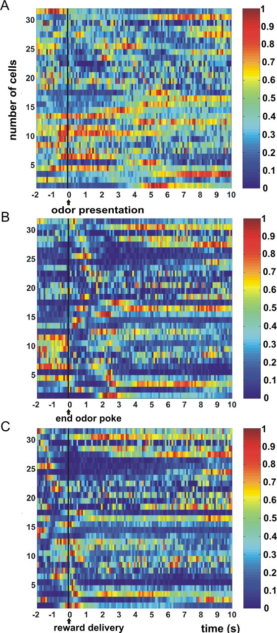
Summary of task-related firing activity of 32 simultaneously recorded OFC neurons during a single session. The horizontal axis denotes time (in seconds), and the vertical axis denotes cell number. Color-coded firing rates were calculated by averaging activity over all rewarded trial types during the session, with bin sizes of 100 ms. A–C, Neural activity is synchronized on odor presentation (A), the end of the odor poke (B), and reward delivery (C). Onset of the waiting period is 1.5 s before reward delivery. Colors indicate firing rates that are normalized relative to the maximum firing rate of each neuron, according to a hotness scale shown on the right. The reward-size variations in firing activity of these cells are used as the basis for studying the ensemble code of reward magnitude.

Before studying population coding principles themselves, we first aimed to assess (1) to what extent the firing-rate variability of single cells is attributable to effects of reward size and (2) whether whole OFC populations exhibit a high or low degree of overall firing-rate variability, regardless of reward size. This was done by calculating two variability measures, namely S_par and S_pop. The mean S_par, indicating the response variability of individual neurons associated with variations in reward size (their tuning curves), was 0.23 for the waiting period and 0.28 for the reward delivery phase (Fig. 4A,B). The mean S_pop, which represents the variability in firing rate across the population regardless of reward size effects, was 0.70 for the waiting period and 0.73 for the reward period (Fig. 4C,D). Similar findings were obtained for the movement period, namely a mean S_par value of 0.25 and a mean S_pop value of 0.76. These results show, first, that there is a high variability of firing rates throughout the population, as illustrated by the high S_pop values throughout the three trial phases. Second, this phenomenon is not matched by a similarly high reward-related variability when individual cells are considered: OFC neurons displayed less variability in their tuning curves to reward size, because for all three task periods the large majority of the cells had values <0.5 (movement period, 76%; n = 518; waiting period, 79%; n = 541; reward period, 76%; n = 520). Apparently, other factors must be present in addition to the reward-modulated response profiles of the individual cells to explain the high variability in the overall population, e.g., differences in baseline firing rate or differences in responsivity during various task phases, although a small subgroup was present with a very high parameter variability (range, 0.9–1.0) in all three task phases.

Figure 4.

Distribution of population variability and parameter variability across orbitofrontal cell populations. A, C, Waiting period; B, D, reward period. Values of population variability across sessions were generally in a high range between 0.4 and 1.0, with means of 0.71 and 0.73 for the waiting and reward periods, respectively. Parameter variability values varied more strongly, spanning the whole range from 0.0 to 1.0 for both periods, with means of 0.23 and 0.28 for the waiting and reward periods, respectively. Similar findings were obtained for the movement period, namely a mean S_par value of 0.25 and a mean S_pop value of 0.76 (data not shown). Note the subgroup of cells with very high parameter variability (0.9–1.0).

In conclusion, whereas firing rates throughout OFC populations are highly variable, modulation of single-cell firing rate that is attributable to reward size is relatively subtle, in line with a previous analysis of single-unit activity in OFC (van Duuren et al., 2007).

Population coding of expected and actual reward magnitude

We will describe first an application of the Bayesian method and template matching in which the magnitude of reward was decoded from ensemble activity in the positively rewarded trial types across the first nine trials of the session, whereas trials 10–15 were used for encoding. During the movement, waiting, and reward periods, the magnitude of reward was decoded from the population activity with a percentage of correct performance significantly above the 1/3 chance level for both methods (one-way ANOVA; p = 0.000 in all three cases). When the decoding score was plotted as a function of the number of cells participating in the reconstruction ensemble, regression analysis showed that with template matching the slope of the decoding curve was significantly positive for all three task phases (p = 0.000 in all cases), meaning that the decoding performance improved with an increasing amount of cells (Fig. 5). The maximum decoding scores were 57% (at n = 30 cells) for the movement period, and 48% (at n = 36 cells) and 76% (n = 36 cells) for the waiting and reward periods, respectively. We also calculated the decoding score for the subgroup of the sessions that did not show a significant difference in response latency between the lowest and highest amount of reward. Reward magnitude could be reconstructed above chance level in this group as well. This finding indicates that significant population coding is present in OFC even in the absence of overt behavioral differences, which corroborates the notion that OFC activity is not necessarily tied to motor behavior and involves a cognitive process.

Figure 5.

Decoding of reward magnitude with template matching: dependence on ensemble size. The horizontal axis indicates the size of the reconstruction ensemble, and the vertical axis indicates the percentage of trials in which reward size was correctly decoded. In the graphs presented here and in Figures 6–7 and 9–10, the horizontal dashed line indicates chance level (33.3%), and dotted lines flanking the curves represent the 95% confidence interval (two times the SE of proportion).

The Bayesian method produced similar although generally somewhat lower decoding scores, with maximum scores of 44% for the movement period and waiting period (at, respectively, n = 26 and n = 24 cells), and 79% for the reward period (at n = 36 cells). Also for this method, regression analysis indicated a significantly rising score with increasing ensemble size for the reward period (p = 0.000). For the waiting and movement period, however, no significant effect was found.

Across all analyses presented here, Bayesian reconstruction and template matching produced similar results for the reward period, whereas for the waiting-anticipation phase the decoding scores were similar or lower for the Bayesian compared with template-matching method. Such differences may be attributable to several factors (see Materials and Methods). Below, we will concentrate on results obtained with template matching.

Temporal resolution of ensemble coding

Because the results indicated reward magnitude to be represented in population activity during task performance in a manner that was consistent across decoding and encoding blocks, the question arose what the temporal resolution of population coding was. This question is relevant for understanding OFC function, because when significant coding is present across short time intervals, this may facilitate rapid decision making and fast behavioral responding. We first asked how the decoding score depends on the width of the time window used for encoding and decoding applied to either the waiting or reward period. To this end, we selected smaller time windows from the overall time windows of the waiting and reward period (1.5 and 10 s, respectively), and calculated the decoding score for time windows of increasing duration. This provides a cumulative measure of the percentage of decoded reward size over time within each trial phase. The waiting period was divided into six time windows that started at 250 ms and went up to 1.5 s, with increments of 250 ms. Time windows used for the reward period were, in addition to the six windows of 250 ms, 2, 3, 4, 5, 6, 8, and 10 s. Regression analysis indicated that with template matching, the percentage of reward amount correctly decoded during the waiting and reward period rose with increasing length of the decoding window, with the slope of the decoding curve being significantly positive (waiting period, p = 0.039; reward period, p = 0.000) (Fig. 6A,B). The maximum decoding scores obtained were 47 and 80% for the waiting and reward periods, respectively. A one-way ANOVA indicated that during the waiting period, only the decoding score obtained with a decoding window of 1.5 s was significantly above chance level (p = 0.001), and furthermore revealed that there was no significant variation between the various window widths. In contrast, during the reward period, all time windows with the exception of the first one differed significantly from chance level (p = 0.000). Furthermore, the first two time windows (i.e., 250 and 500 ms) had a significantly lower decoding score than the final six time windows (i.e., 3, 4, 5, 6, 8, and 10 s). Thus, for a significant success rate in decoding actual reward size, only a short time segment (∼0.5 s) of the population response is needed, whereas the time segment needed for a significant success rate in decoding expected reward is somewhat longer, namely 1.5 s.

Figure 6.

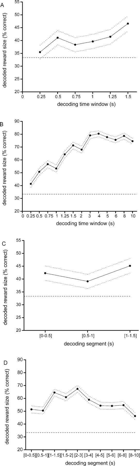
Decoding of reward magnitude within specific trial phases. The size of the reconstruction ensemble was 37 neurons. A, B, Decoding score using time windows of increasing duration for the waiting (A) and the reward delivery (B) periods. The horizontal axis shows the size of the time window (in seconds) from which spikes were taken for reconstruction, and the vertical axis shows the percentage of correctly decoded trials. C, D, The decoding success for consecutive temporal segments in the waiting and reward periods, respectively. The horizontal axis now shows the time segment of trial phase used for reconstruction. In C, the decoding segments are the intervals (0–0.5), (0.5–1.0), and (1.0–1.5) s relative to fluid poke onset. In D, the segments are (0–0.5), (0.5–1.0), (1.0–1.5), (1.5–2.0), (2.0–3.0), (3.0–4.0), (4.0–5.0), (5.0–6.0), (6.0–8.0), and (8.0–10.0) s relative to reward delivery.

We next asked how the decoding capacity of the population varies over time across consecutive segments of the waiting and reward periods. This question probes the time resolution at which significant reward-predictive information is represented across consecutive time segments of a behavioral task phase. Therefore the percentage of correctly decoded reward amount was calculated for successive time segments across the entire length of the overall time windows of the waiting and reward period. Thus, a sequential method was adopted instead of the cumulative method used above. For the waiting period, we used three consecutive time segments of 500 ms; for the reward period, decoding was calculated during the first 2 s in time segments of 500 ms, followed by four time segments of 1 s, and the final two segments of 2 s. During both the waiting and reward period, regression analysis and one-way ANOVA did not show a significant variation in decoding success, indicating that the amount of decodable information did not significantly differ across the various time segments within this task period (Fig. 6C,D).

Development of population coding during task progression

Because the data on response times and the number of trials per reinforcer indicated that in the course of a session animals generated predictions about response outcome and learned to discriminate between different amounts of reward, we addressed the question how the representation of reward magnitude by population activity evolved in the course of learning during a session. To this end, the decoding block was divided into four consecutive two-trial blocks (block 1, trials 1 and 2; block 2, trials 3 and 4, block 3, trials 5 and 6; block 4, trials 7 and 8), and decoding was compared between these four blocks. Trial numbers 10–15 were used for encoding (as above). In all four trial blocks and for both the waiting and reward period, reward magnitude was decoded from the population activity above chance level (one-way ANOVA; p = 0.000). Regression analysis indicated for the waiting period a significant slope of the decoding score for blocks 2, 3, and 4. Decoding with the first trial block differed significantly from all three other blocks, with an improvement in decoding score as the task progressed, except for the final (fourth) trial block. The second block did not differ from the third block, whereas the third block differed significantly from the fourth (Fig. 7A). During the reward period, all blocks showed a significant slope of the decoding curves. Furthermore, the decoding curves differed significantly between the first and the second blocks and the third versus the fourth, with an improvement of decoding success; the second block did not differ from the third block (Fig. 7B). An additional two-way ANOVA indicated no interaction between cell group size and trial block.

Figure 7.

Changes in reconstruction success across consecutive blocks of learning trials. A, B, The percentage of correctly decoded reward amounts per trial block for the waiting and reward periods, respectively. In view of the reliability of reconstruction because of the low number of trials per trial block, a reconstruction ensemble of 26 neurons was used, which was the minimal number of neurons present in all sessions. The horizontal axis indicates the size of the reconstruction ensemble. In A and B, encoding vectors were obtained from trials 10–15 for each reward size. To maintain clarity, SEs of proportion are not shown, but these values were generally comparable to those in Fig. 4. C, D, Mean decoding success for the encoding by late trials (i.e., 10–15) and its temporal mirror image (encoding by early trials; i.e., 1–6) for the waiting (C) and reward (D) periods. The abscissa denotes the proximity of decoding trials to the encoding block; the larger the decoding block number, the closer that block is to the encoding block. Error bars indicate SEM values.

The trial-block sequence observed for the waiting period, in which block 1 is flat, whereas the blocks 2, 3, and 4 show increasing decoding with an augmenting number of cells as indicated by the regression analysis, suggests that OFC ensembles have only a weak predictive ability at the beginning of the session (the first block), which is already consistently present in small subsets of neurons. At this time in the session, the decoding score does not rise with an increasing amount of cells; adding more cells to the ensemble adds both “confirmatory” and “conflicting” evidence about the predicted reward size. However, the ability to predict reward size increases with experience over trial blocks (blocks 2, 3, and 4), and the decoding score now comes to depend on the number of cells that participate in the ensemble, as indicated by the regression analysis. This means that at this point, the code has developed in a more consistent and redundant manner within OFC, with less conflicting neural evidence.

Nonspecific drift across trials as a possible confounding factor

The increased decoding success found for later trial blocks relative to earlier ones may be explained either by a learning effect or by a nonspecific “drift” in ensemble responses over trials, because the final block of five trials (i.e., trials 10–15) was used for the encoding. To check whether the latter, confounding possibility would apply, we compared the two-trial decoding blocks when the encoding block was situated at the session end (trials 10–15) with two-trial blocks when the encoding block was situated at the start of the session (encoding block, trials 1–6; decoding block 1, trials 7 and 8; block 2, trials 9 and 10, block 3, trials 11 and 12; block 4, trials 13 and 14). Because outcome-prediction learning is expected to be unevenly distributed across trials (with a rapid decrease in go-responses for the quinine and nonrewarded trials early in the session), it is predicted that these decoding procedures should yield separate or at most partially overlapping curves for the waiting period if the progressive change in decoding is indeed attributable to learning. Thus, the curve with encoding by late trials should rise more steeply and then stabilize compared with its temporal mirror image. As illustrated in Figure 7C, showing the average of the decoding curves per trial block for the waiting period (as in Fig. 7A), the curves indeed confirmed this prediction. A one-way ANOVA (p < 0.05) indicated that for the waiting period all trial blocks of the two different encoding conditions differed significantly from each other, except for the fourth block. For the reward period, in which additional learning may or may not take place, the first and the fourth trial block differed significantly between the two encoding conditions, with a steeper rise across trial blocks when the encoding block was at the session end (Fig. 7D).

Altogether, these results indicate that progressive learning of odor–reward associations coupled to motor responses is accompanied by a quick rise in population coding of expected reward magnitude during the waiting period, followed by relative stabilization: a time course not attributable to nonspecific drift. An additional learning-related increase in population coding appears to take place in the reward period, although this effect is less strong.

Temporal specificity of reward coding within trials

In principle, it is possible that population activity does not code reward magnitude only during the single trial phases for which it was examined. For example, information about reward amount may be carried over from one trial period to the next, similar to “delay cells” in, e.g., monkey dorsolateral prefrontal cortex (Funahashi et al., 1989). In contrast, one may hypothesize that this type of information is coded by specific neuronal groups, active during a particular trial phase, without any working memory-like activity or carryover to the next trial phase. To examine this, the time window in which decoding was calculated for the movement period (1 s) was shifted in time with a step size of 0.25 s relative to the onset of this period, whereas the time window for encoding remained unchanged. For each step, the amount of decoding success was recalculated. If coding of expected reward magnitude is confined to periods around such a specific event, decoding is expected to approximate chance level shortly before and after the event period.

As expected, Figure 8A shows that during the movement period, the decoding score for the expected magnitude of reward was highest when no time shift was applied (Δt = 0). For both negative and positive shifts in time, the decoding scores decreased rapidly to chance level: the scores differed significantly from the decoding score calculated at time t = 0 (i.e., lower than two times the confidence interval at time t = 0) in the period after +0.5 and before −0.5 s, suggesting a large segregation with population coding during earlier and later trial phases.

Figure 8.

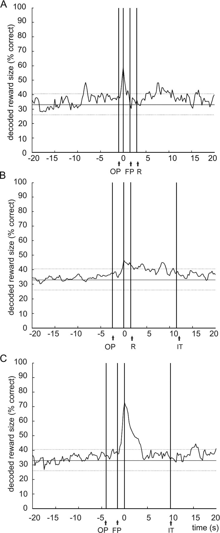
A–C, Temporal specificity of coding reward size assessed with reference to the movement (A), the waiting (B), and the reward delivery (C) periods. A reconstruction ensemble of 26 cells was used, and the decoding time windows were 1 s for the movement period and 1.5 s for both the waiting and reward periods. The abscissa plots the time (in seconds) by which the decoding vector was shifted in 0.25 s steps relative to the encoding vector, with t = 0 at the offset of odor sampling (A), the onset of fluid poking (B), and reward delivery (C). The decoding score is significantly lower (i.e., lower than 2 times confidence interval) compared with time t = 0 before −0.5 s and after 0.5 s for the movement period. For the waiting period, the decoding score is significantly lower before −0.25 s and after +2.0 s, for the reward delivery period before −0.25 s and after +0.75 s. Parallel vertical lines indicate the average onset of odor poking (OP), fluid poke onset (FP), reward delivery (R), and onset of the intertrial interval (IT). For reasons of clarity, SEs of proportion are not shown. Horizontal lines represent two times the SD above or below chance level.

The same procedure was applied for the waiting period, having a time frame of 1.5 s (Fig. 8B). Relative to the maximal decoding score obtained when no time shift was applied, the score dropped slightly within +1.5 s after event onset, but only slowly returned to chance level after the +1.5 s period. The decoding score differed significantly from the decoding score at time t = 0 in the period after +2.0 s. The slow decay is likely related to a certain consistency in ensemble firing patterns across the phases of expected versus actual reward. In contrast, negative shifts in time produced a steep decrease in decoding score; the decoding scores were found to be significantly lower compared with the score at time t = 0 in the period before −0.25 s.

For the reward period, a time window of 1.5 s was applied as well (Fig. 8C). Also in this case, the percentage of correct decoding decreased relatively slowly within +3.0 after event onset. Shifting leftwards, the decoding scores were found to be significantly lower compared with the score at time t = 0 in the period before −0.25 s, again suggesting a segregation with earlier trial phases, and in the period after +0.75 s. We also examined a time window of 10 s for the reward period (data not shown), which provided a comparable result, although the decay slopes for positive and negative shifts in time were less steep because an overlap between the encoding and decoding window remained until boundaries of +10 or −10 s were reached by time shifting.

We performed an additional analysis to examine whether the template for encoding the magnitude during the reward phase can be used for decoding the expected magnitude during the anticipatory period, and how such matching develops as learning progresses. If significant matching exists, this would confirm the consistency of the ensemble pattern across the two trial phases. To this end, we used the reward period for encoding and the firing activity during the anticipatory period for decoding. We divided the decoding block into four consecutive two-trial blocks (block 1, trial 1 and 2; block 2, trial 3 and 4, block 3, trial 5 and 6; block 4, trial 7 and 8) and compared decoding between these four blocks. Trial numbers 10–15 were used for encoding. This analysis showed that in all four trial blocks, there was a modest but significant decoding of reward magnitude (p < 0.05), but the fourth block showed a significantly lower decoding score with respect to the previous three trial blocks (mean ± SEM, block 1, 38.5 ± 0.2%; block 2, 38.6 ± 0.2%; block 3, 38.3 ± 0.3%; block 4, 35.3 ± 0.4%) (Fig. 9). This indicates that initially the representation of reward magnitude is similar between these two task phases, meaning that in this phase of the learning task there is a large overlap in reward-related ensemble patterns of the anticipatory and delivery phases. During later stages of the task, however, the neural representations of the reward and anticipatory phases become more differentiated. Apparently, during task progression, the activity of the cells involved in magnitude representation shows a marked change after the transition from the anticipatory to the delivery phase, which can be viewed as a partial decorrelation of the code.

Figure 9.

Decoding of reward size during the waiting period when spike vectors from the reward delivery period were used for encoding. A reconstruction ensemble of 26 neurons was used, and the decoding time window was 1.5 s. For all four two-trial blocks (see also Fig. 7), a decoding score was obtained significantly above chance level. The fourth trial block showed a significantly lower decoding score with respect to the previous three trial blocks. Error bars indicate SEM values.

In conclusion, whereas the ensemble firing patterns in the movement phase do not show marked carryover to adjacent phases, a notable consistency in coding exists between the waiting and delivery periods. This consistency is also expressed when using the reward phase for encoding and the waiting period for decoding, especially in the early phases of learning. As regards the lack of consistency or carryover between the earlier trial phases (odor sampling, movement, and waiting periods), it is of note that our data are at variance with a view in which reward-magnitude information would be maintained by the OFC throughout various trial phases in a working memory-like manner, as exemplified by dorsolateral prefrontal neurons in primates showing enhanced firing during delay intervals (Leon and Shadlen, 1999; Fuster et al., 2000; Wallis et al., 2001).

Contribution of individual cells to coding of reward magnitude

Decoding expressed as a function of cell number (Fig. 5) does not reveal individual contributions of cells to the population code of reward magnitude, because in this calculation decoding scores were averages across groups of randomly selected neurons. To assess the contribution of individual cells to the decoding success, we computed for all recorded neurons the difference in the percentage of decoded information when a specific cell was added to a group of five neurons randomly selected from the same session. Apart from the consideration that single cells may contribute reasonably to coding by such a relatively small group, this size was chosen arbitrarily. For each cell, this calculation was done 100 times, each time with a new randomly selected group of five additional neurons. This procedure showed that during the movement period, 32% of the cells (n = 219) made a minimal contribution to the decoding capacity of the population (between −0.5 and 0.5%). Thirty-five percent of the cells (n = 239) made a positive contribution (>0.5%) to successful reconstruction (average contribution ± SEM, 6.5 ± 0.4%), whereas 33% (n = 225) contributed negatively (greater negative contribution than −0.5%) with an average of 4.3 ± 0.4%, implying that addition of these cells led to a decrease in correct decoding. The positive contribution was found to be significantly higher than the negative one (unpaired t test; p = 0.000). Three percent of the cells (n = 20) made a contribution of >15% to the decoding score (average, 20.1 ± 0.9%), whereas 1.5% (n = 10) made a large negative contribution (greater negative contribution than −15%) that was significantly lower than the positive contribution, namely 17.2 ± 0.7% (unpaired t test; p < 0.05).

During the waiting period, 26% of the cells (n = 178) made a minimal contribution to the decoding capacity of the population, whereas 40% of the cells (n = 273) made a positive contribution (>0.5%) to successful reconstruction (average contribution ± SEM, 5.1 ± 0.3%). Thirty-four percent (n = 232) contributed negatively with an average of 4.5 ± 0.3%. The average positive contribution, however, did not differ significantly from the negative one. Examination of the number of cells that made a contribution of >15% to the decoding score (either positive or negative) showed that 2% of the cells (n = 14) contributed positively to the decoding score with an average of 21.4 ± 1.9%, whereas 0.6% (n = 2) made a negative contribution that was significantly lower than the positive contribution, namely 20.5 ± 1.4% (unpaired t test; p < 0.05).

During the reward period, 15% of the cells (n = 102) made a minimal contribution, whereas 50% (n = 342) and 35% (n = 239) contributed in a positive (average contribution ± SEM, 6.7 ± 0.4%) and negative (4.0 ± 0.4%) manner, respectively. The positive contribution was found to be significantly higher than the negative one (unpaired t test; p = 0.000). Six percent of the cells (n = 41) contributed >15% to the decoding score in a positive manner (23.4 ± 1.3%), whereas 0.4% (n = 3) was found to contribute >15% in a negative manner (19.0 ± 1.3%). Also in this case, the negative contribution was significantly lower compared with the positive one (unpaired t test; p = 0.000).

In addition, cells that showed the largest variability in their response toward reward magnitude (i.e., parameter variability between 0.9 and 1.0) (Fig. 4) were removed from the entire population of neurons, and the decoding score for the remaining population was recalculated (number of neurons removed: movement period, n = 69; waiting period, n = 62; reward period, n = 79). This resulted in decoding scores that did not differ significantly from the decoding curves obtained using the entire population.

In summary, for all three task phases we found large subgroups of cells making modest to large contributions to the population representation of reward magnitude, both positive and negative. These results confirm the notion (see also Fig. 5) that reward magnitude is coded in a distributed and redundant manner. Although subsets making positive contributions generally outweighed the “negative contributors,” it is striking to note that so many negative contributors were found, which implies that many cells generated firing patterns that were inconsistent with respect to reward size across encoding and decoding trials. This notion is especially relevant when framed in the context of the problem, how target areas of the OFC “read out” its population activity (cf. Pouget et al., 1998, 2000). If one considers previously acquired results indicating that single OFC cells code information on, e.g., expected reward size or delay until reward delivery, one may be inclined to think that such single-cell signals can be easily read out and used by a target area (such as the striatum) for further computations, but this is a simplification of the problem if one reflects on the current results. Namely, there appear to be many other OFC neurons in the vicinity of the specifically tuned one that may contribute “noise” and/or even make a negative contribution to the population code, relative to that neuron. Despite this readout problem, the present results also show that target areas of the OFC, if endowed with proper processing circuitry, can extract significant information on predicted and actual reward sizes from OFC population output, even in early phases of learning.

Erroneous go-trials: quinine responses versus sucrose responses

During the task, animals learned to avoid negative response outcomes, as visible by the low number of go-responses to quinine (“false alarms”). We examined whether reconstruction of reward size could be achieved by using the quinine-reinforced go trials for encoding and positively reinforced trials for decoding. If, as hypothesized, the decoding success during the waiting period is truly attributable to the expectation and processing of reward information, reconstruction for quinine versus sucrose trials should deliver a random decoding score (i.e., close to 33.3% correct). Alternatively, however, some correct reconstruction may occur because of the expected and actual volume of liquid ingested, regardless of the quality of the reinforcer (the volume of quinine solution was equal to the middle-sized sucrose reward, viz. 150 μl). If this is the case, a significant decoding success is predicted to occur during both the waiting and reward period. For this calculation, all available quinine trials were used for encoding, whereas for decoding, the sucrose trials 1–9 were used. Figure 10 shows that for both the waiting and reward period, the decoding score for reward size was around chance level regardless of ensemble size, confirming that decoding success in Figures 5–8 is attributable to reward quality. Using only trials with 0.15 ml of sucrose reward to calculate the decoding score when quinine was used for encoding yielded a similar result, namely a percentage correct at chance level. This furthermore indicates that variations in population activity observed during these two trial periods are not attributable to licking behavior of the animal, because in both trial types, reinforcement was consumed by the animals [for consistent single-unit results in relation to licking, see also van Duuren et al. (2007)].

Figure 10.

Decoding scores for reward size (sucrose solution) when spike vectors from quinine trials (amount of 0.15 ml) were used for encoding. A, B, Results for the waiting (A) and reward delivery (B) periods. During both task phases, the decoding success for reward size is around chance level, which indicates that the population activity represents reward quality and not volume of liquid reinforcer. When only trials with 0.15 ml of sucrose reward were used for decoding, a similar result was obtained: the decoding score was around chance level. To maintain clarity, SEs of proportion are not shown, but these values were generally comparable to those in Figure 4.

Discussion

The involvement of the OFC in decision making has been primarily examined by lesion experiments or single-unit recordings made during task performance. Based on these studies, the OFC has been proposed to integrate learned associative information with action plans to guide behavior in a flexible manner (Dias et al., 1996; Schoenbaum et al., 1998, 2006; Gallagher et al., 1999; Tremblay and Schultz, 1999; Baxter et al., 2000; Ramus and Eichenbaum, 2000; O'Doherty et al., 2001; Fellows and Farah, 2003; Plassmann et al., 2007). However, it has remained uncertain how behaviorally meaningful information is represented by OFC population activity when adaptive behavior is required. By performing ensemble recordings while animals learned odor-reinforcer associations, we showed that information about reward magnitude could be decoded from OFC population activity during three trial phases, viz. when animals generated movements directed at reward, during waiting for reward, and when reward is received. Comparing reconstruction success between these periods, the decoding score was highest for the reward period; apparently, population activity is more discriminative with respect to varying reward amount when based on the actual presence of reward than based on predictive information derived from odor cues. It can be argued that during the reward period OFC receives other information in addition to valuation inputs, viz. sensorimotor feedback related to liquid ingestion per se, but this does not explain the random decoding score when quinine trials were used for encoding and sucrose trials for decoding. Despite this argument, population activity during the reward period may be determined by other processes in addition to reward appraisal, e.g., tasting, which is inextricably linked to it. The lower decoding scores observed in the waiting period may be explained by the fact that animals were in the process of learning novel odor–reward contingencies, which is supported by the rapidly rising decoding scores during progressive trial blocks (Fig. 7A). Another, not mutually exclusive explanation holds that no specific task requirement to obtain a high reward amount was present, possibly leading to a relatively weak demand on the system's computational resources to represent reward magnitude. Although animals are immobile during the waiting period, we cannot rule out the possibility that, for example, small changes in posture may influence neural activity within this period. Changes in attention, intimately linked to reward expectation, might also occur, but it is unlikely that the results would be confounded by attentional factors, because OFC has not been implicated in attention per se, and attentional modulation of firing responses would not explain the difference between coding for sucrose versus quinine.

Development of population representation of reward magnitude

Despite a limited number of trials, we were able to demonstrate for the first time an increasing success in reconstructing reward size during task progression. Across trials, animals learned to discriminate between different reward sizes, and hence this increase in correct predictions of reward size may reflect learning-related changes. Indeed, testing the alternative hypothesis of a nonspecific drift in ensemble response over trials indicated a learning effect, because the forward curve (late encoding) exhibited a steeper rise and a modest decay as trials progressed compared with the more gradually rising backward curve (early encoding). Increasing decoding scores were also found for the reward period, during which the forward curve rose more steeply than the backward curve. This may be explained by an adaptation in ensemble activity correlating to an additional learning process. An initial number of trials in which the various rewards are actually assessed by the animal may be needed to train the population to distinguish them. Admittedly, however, our task did not include requirements to assess this type of learning explicitly.

Variability and redundancy of the representation of reward magnitude

Mean firing rates across the population showed a high degree of variability, consistent with a great variability in activity levels during specific trial phases. Despite this, individual cells showed a vast range of variability values toward reward magnitude. Thus, the great overall variability in neural activity in the population was only partially matched by differences in individual neuronal responses to reward size (tuning), suggesting a limited degree of the variability in reward-magnitude representations.

Decoding scores were weakly dependent on the ensemble size used for reconstruction (Fig. 5), and removing the fraction of cells demonstrating high parameter variability did not significantly alter the score, implying that the absence of these cells did not result in a significant loss of reward-predictive information. Considering individual cell contributions to the performance of a small ensemble (n = 5), only a few cells made a substantial (>15%) positive contribution to the decoding score, whereas a large number of cells made small to moderate (0.5–15%) contributions. These results are consistent with the concept of redundant coding, meaning that reward magnitude is coded in a broadly, distributed manner within OFC, and losses of considerable subpopulations will not lead to a strongly degraded output signal. That the amount of cells making either a negative or positive contribution in the waiting period is about equal is compatible with a gradual development of reward-predictive population activity during learning and a moderate decoding success for this phase. Such negative contributions may easily arise when spike patterns show a high variability across trials inconsistent with variations in upcoming reward size.

Temporal specificity of reward coding within and across trial phases

In addition to decoding reward size within specific temporal phases of learning trials, we also studied whether representations remain detectable at a finer time resolution. When reconstruction time windows in the reward phase were gradually increased, decoding performance tended to stabilize after ∼3 s, indicating that significant representations can be detected at a time resolution finer than entire trial phases. For the waiting period, however, 1.5 s was needed to reach a significant decoding score (Fig. 6A,B). Analysis of decoding performance across successive time segments of both trial phases (Fig. 6C,D) showed that decoding success did not greatly vary with the temporal position of the segment in each phase. However, this preserved decoding capacity for small intervals within trial phases does not imply that the same OFC ensemble would code reward information consistently throughout the trial, as shown by a decreased success rate when decoding frames were shifted in time (Fig. 8). For the waiting period, a shift toward the right resulted in a slow decrease in decoding success, but a shift in the reverse direction quickly brought decoding to chance level. Apparently, cell groups representing reward-predictive information during this period do not generate similar representations during earlier trial phases, e.g., odor sampling. A similar lack of carryover was found for the movement phase. In addition, no consistent decoding of reward frames was found during the intertrial interval, arguing against a maintenance of reward representations by the same neurons between consecutive trials.

Population coding of reward information in OFC: functional implications

Only a few studies have related ensemble activity to reward processing in OFC. In an odor-discrimination task, Schoenbaum and Eichenbaum (1995) found that during odor sampling, ensembles coded odor identity and expectation of reward presented in the following trial. This pioneering study differs from ours because we focused on outcome prediction on the basis of a cue within the same trial, on temporal coding specificity within trials, and on dynamic adaptation during learning of novel associations. Gutierrez et al. (2006) demonstrated population activity discriminating water and sucrose rewards, both when animals anticipated reward and when they tasted it. In this experiment, predictive cues were absent and animals were allowed to drink water, followed by a session of sucrose-solution intake. Such a coarse time indicator for outcome anticipation may be confounded by drifts in ensemble coding over session time, and differential anticipatory activity may be confounded by differences in motor preparation. An advantage of a parametrically varied reward is that such possible confounds can be controlled for because animals perform similar behavior to obtain different reinforcers.

The overall concept of OFC population coding emerging from the present findings holds that representations of reinforcer quality and magnitude are broadly distributed across ensembles and are characterized by a high, subsecond time resolution. These properties cannot be deduced by other techniques such as single-cell recording or functional magnetic resonance imaging. Combining the current results with single-unit results suggesting task-phase specific coding (Simmons and Richmond, 2008), neural coding in OFC appears highly specific and well articulated for the temporal phase an animal is in toward achieving a goal, whereas reward parameters as magnitude are expressed more as modulatory signals, rather than being main determinants of firing rate. When considering how such parallel-distributed signals may be read out by neuronal populations in target areas of OFC, it is noteworthy that significant readout of reward-predictive information can occur by processing output from small groups of neurons and of narrow time segments within trials, enabling rapid decision making. If target populations assume a particular functional organization such as a continuous attractor, they have the natural capacity, at least in principle, to read out OFC output efficiently by template matching or Bayesian reconstruction (Pouget et al., 1998; Zhang et al., 1998; Wu and Amari, 2005).

References

- Baeg EH, Kim YB, Huh K, Mook-Jung I, Kim HT, Jung MW. Dynamics of the population code for working memory in the prefrontal cortex. Neuron. 2003;40:177–188. doi: 10.1016/s0896-6273(03)00597-x. [DOI] [PubMed] [Google Scholar]
- Baxter MG, Parker A, Lindner CCC, Izquierdo AD, Murray EA. Control of response selection by reinforcer value requires interaction of amygdala and orbital prefrontal cortex. J Neurosci. 2000;20:4311–4319. doi: 10.1523/JNEUROSCI.20-11-04311.2000. [DOI] [PMC free article] [PubMed] [Google Scholar]
- Bialek W, Rieke F, de Ruyter van Steveninck RR, Warland D. Reading a neural code. Science. 1991;252:1854–1857. doi: 10.1126/science.2063199. [DOI] [PubMed] [Google Scholar]
- Dias R, Robbins TW, Roberts AC. Dissociation in prefrontal cortex of affective and attentional shifts. Nature. 1996;380:69–72. doi: 10.1038/380069a0. [DOI] [PubMed] [Google Scholar]
- Fellows LK, Farah MJ. Ventromedial frontal cortex mediates affective shifting in humans: evidence from a reversal learning paradigm. Brain. 2003;126:1830–1837. doi: 10.1093/brain/awg180. [DOI] [PubMed] [Google Scholar]
- Földiák P. The ‘ideal homunculus’: statistical inference from neural population responses. In: Eeckman F, Bower J, editors. Computation and neural systems. Norwell, MA: Kluwer Academic; 1993. pp. 55–60. [Google Scholar]
- Funahashi S, Bruce CJ, Goldman-Rakic PS. Mnemonic coding of visual space in the monkey's dorsolateral prefrontal cortex. J Neurophysiol. 1989;61:331–349. doi: 10.1152/jn.1989.61.2.331. [DOI] [PubMed] [Google Scholar]
- Fuster JM, Bodner M, Kroger JK. Cross-modal and cross-temporal association in neurons of frontal cortex. Nature. 2000;405:347–351. doi: 10.1038/35012613. [DOI] [PubMed] [Google Scholar]
- Gallagher M, McMahan RW, Schoenbaum G. Orbitofrontal cortex and representation of incentive value in associative learning. J Neurosci. 1999;19:6610–6614. doi: 10.1523/JNEUROSCI.19-15-06610.1999. [DOI] [PMC free article] [PubMed] [Google Scholar]
- Georgopoulos AP, Schwartz AB, Kettner RE. Neuronal population coding of movement direction. Science. 1986;233:1416–1419. doi: 10.1126/science.3749885. [DOI] [PubMed] [Google Scholar]
- Gothard KM, Skaggs WE, Moore KM, McNaughton BL. Binding of hippocampal CA1 neural activity to multiple reference frames in a landmark-based navigation task. J Neurosci. 1996;16:823–835. doi: 10.1523/JNEUROSCI.16-02-00823.1996. [DOI] [PMC free article] [PubMed] [Google Scholar]
- Gray CM, Maldonado PE, Wilson M, McNaughton B. Tetrodes markedly improve the reliability and yield of multiple single-unit isolation from multi-unit recordings in cat striate cortex. J Neurosci Methods. 1995;63:43–54. doi: 10.1016/0165-0270(95)00085-2. [DOI] [PubMed] [Google Scholar]
- Gutierrez R, Carmena JM, Nicolelis MAL, Simon SA. Orbitofrontal ensemble activity monitors licking and distinguishes among natural rewards. J Neurophysiol. 2006;95:119–133. doi: 10.1152/jn.00467.2005. [DOI] [PubMed] [Google Scholar]
- Hikosaka K, Watanabe M. Delay activity of orbital and lateral prefrontal neurons of the monkey varying with different rewards. Cereb Cortex. 2000;10:263–271. doi: 10.1093/cercor/10.3.263. [DOI] [PubMed] [Google Scholar]
- Ichihara-Takeda S, Funahashi S. Reward-period activity in primate dorsolateral prefrontal and orbitofrontal neurons is affected by reward schedules. J Cog Neurosci. 2006;18:212–226. doi: 10.1162/089892906775783679. [DOI] [PubMed] [Google Scholar]
- Laubach M, Wessberg J, Nicolelis MA. Cortical ensemble activity increasingly predicts behaviour outcomes during learning in a motor task. Nature. 2000;405:567–571. doi: 10.1038/35014604. [DOI] [PubMed] [Google Scholar]
- Lehky SR, Sejnowski TJ. Neural model of stereoacuity and depth interpolation based on a distributed representation of stereo disparity. J Neurosci. 1990;10:2281–2299. doi: 10.1523/JNEUROSCI.10-07-02281.1990. [DOI] [PMC free article] [PubMed] [Google Scholar]
- Leon MI, Shadlen MN. Effect of expected reward magnitude on the response of neurons in the dorsolateral prefrontal cortex of the macaque. Neuron. 1999;24:415–425. doi: 10.1016/s0896-6273(00)80854-5. [DOI] [PubMed] [Google Scholar]
- Lipton PA, Alvarez P, Eichenbaum H. Crossmodal associative memory representations in rodent orbitofrontal cortex. Neuron. 1999;22:349–359. doi: 10.1016/s0896-6273(00)81095-8. [DOI] [PubMed] [Google Scholar]
- Louie K, Wilson MA. Temporally structured replay of awake hippocampal ensemble activity during rapid eye movement sleep. Neuron. 2001;29:145–156. doi: 10.1016/s0896-6273(01)00186-6. [DOI] [PubMed] [Google Scholar]
- Narayanan NS, Kimchi EY, Laubach M. Redundancy and synergy of neuronal ensembles in rat motor cortex. J Neurosci. 2005;25:4207–4216. doi: 10.1523/JNEUROSCI.4697-04.2005. [DOI] [PMC free article] [PubMed] [Google Scholar]
- O'Doherty J, Kringelbach ML, Rolls ET, Hornak J, Andrews C. Abstract reward and punishment in the human orbitofrontal cortex. Nat Neurosci. 2001;4:95–102. doi: 10.1038/82959. [DOI] [PubMed] [Google Scholar]
- Padoa-Schioppa C, Assad JA. Neurons in the orbitofrontal cortex encode economic value. Nature. 2006;441:223–226. doi: 10.1038/nature04676. [DOI] [PMC free article] [PubMed] [Google Scholar]
- Paxinos G, Watson C. The rat brain in stereotaxic coordinates. New York: Academic; 1996. [DOI] [PubMed] [Google Scholar]
- Perez-Orive J, Mazor O, Turner GC, Cassenaer S, Wilson RI, Laurent G. Oscillations and sparsening of odor representations in the mushroom body. Science. 2002;297:359–365. doi: 10.1126/science.1070502. [DOI] [PubMed] [Google Scholar]
- Plassmann H, O'Doherty J, Rangel A. Orbitofrontal cortex encodes willingness to pay in everyday economic transactions. J Neurosci. 2007;27:9984–9988. doi: 10.1523/JNEUROSCI.2131-07.2007. [DOI] [PMC free article] [PubMed] [Google Scholar]
- Pouget A, Zhang K, Deneve S, Latham PE. Statistically efficient estimation using population coding. Neural Comput. 1998;10:373–401. doi: 10.1162/089976698300017809. [DOI] [PubMed] [Google Scholar]
- Pouget A, Dayan P, Zemel R. Information processing with population codes. Nat Rev Neurosci. 2000;1:125–132. doi: 10.1038/35039062. [DOI] [PubMed] [Google Scholar]
- Ramus SJ, Eichenbaum H. Neural correlates of olfactory recognition memory in the rat orbitofrontal cortex. J Neurosci. 2000;20:8199–8208. doi: 10.1523/JNEUROSCI.20-21-08199.2000. [DOI] [PMC free article] [PubMed] [Google Scholar]
- Ramus SJ, Davis JB, Donahue RJ, Discenza CB, Waite AA. Interaction between the orbitofrontal cortex and the hippocampal memory system during the storage of long-term memory. Ann N Y Acad Sci. 2007;1121:216–231. doi: 10.1196/annals.1401.038. [DOI] [PubMed] [Google Scholar]
- Rieke F, Warland D, de Ruyter van Steveninck R, Bialek W. Spikes: exploring the neural code. Cambridge, MA: MIT; 1997. [Google Scholar]
- Roesch MR, Olson CR. Neuronal activity to reward value and motivation in primate frontal cortex. Science. 2004;304:307–310. doi: 10.1126/science.1093223. [DOI] [PubMed] [Google Scholar]
- Roesch MR, Taylor AR, Schoenbaum G. Encoding of time-discounted rewards in orbitofrontal cortex is independent of value representation. Neuron. 2006;51:509–520. doi: 10.1016/j.neuron.2006.06.027. [DOI] [PMC free article] [PubMed] [Google Scholar]
- Rolls ET, Tovee MJ. Sparseness of the neuronal representation of stimuli in the primate temporal visual cortex. J Neurophysiol. 1995;73:713–726. doi: 10.1152/jn.1995.73.2.713. [DOI] [PubMed] [Google Scholar]
- Sanger TD. Probability density estimation for the interpretation of neural population codes. J Neurophysiol. 1996;76:2790–2793. doi: 10.1152/jn.1996.76.4.2790. [DOI] [PubMed] [Google Scholar]
- Schoenbaum G, Eichenbaum H. Information coding in the rodent prefrontal cortex. II. Ensemble activity in orbitofrontal cortex. J Neurophysiol. 1995;74:751–762. doi: 10.1152/jn.1995.74.2.751. [DOI] [PubMed] [Google Scholar]
- Schoenbaum G, Chiba AA, Gallagher M. Orbitofrontal cortex and basolateral amygdala encode expected outcomes during learning. Nat Neurosci. 1998;1:155–159. doi: 10.1038/407. [DOI] [PubMed] [Google Scholar]
- Schoenbaum G, Chiba AA, Gallagher M. Neural encoding in orbitofrontal cortex and basolateral amygdala during olfactory discrimination learning. J Neurosci. 1999;19:1876–1884. doi: 10.1523/JNEUROSCI.19-05-01876.1999. [DOI] [PMC free article] [PubMed] [Google Scholar]
- Schoenbaum G, Setlow B, Saddoris MP, Gallagher M. Encoding predicted outcome and acquired value in orbitofrontal cortex during cue sampling depends upon input from the basolateral amygdala. Neuron. 2003;39:855–867. doi: 10.1016/s0896-6273(03)00474-4. [DOI] [PubMed] [Google Scholar]
- Schoenbaum G, Setlow B, Saddoris MP, Gallagher M. Encoding changes in orbitofrontal cortex in reversal-impaired aged rats. J Neurophys. 2006;95:1509–1517. doi: 10.1152/jn.01052.2005. [DOI] [PMC free article] [PubMed] [Google Scholar]
- Simmons JM, Richmond BJ. Dynamic changes in representations of preceding and upcoming reward in monkey orbitofrontal cortex. Cereb Cortex. 2008;18:93–103. doi: 10.1093/cercor/bhm034. [DOI] [PubMed] [Google Scholar]
- Thiel A, Greschner M, Eurich CW, Ammermüller J, Kretzberg J. Contribution of individual retinal ganglion cell responses to velocity and acceleration encoding. J Neurophysiol. 2007;98:2285–2296. doi: 10.1152/jn.01342.2006. [DOI] [PubMed] [Google Scholar]
- Thorpe SJ, Rolls ET, Maddison S. The orbitofrontal cortex: neuronal activity in the behaving monkey. Exp Brain Res. 1983;49:93–115. doi: 10.1007/BF00235545. [DOI] [PubMed] [Google Scholar]
- Tremblay L, Schultz W. Relative reward preference in primate orbitofrontal cortex. Nature. 1999;398:704–708. doi: 10.1038/19525. [DOI] [PubMed] [Google Scholar]
- van Duuren E, Nieto-Escámez FA, Joosten RNJMA, Visser R, Mulder AB, Pennartz CMA. Neural coding of reward magnitude in the orbitofrontal cortex of the rat during a five-odor discrimination task. Learn Mem. 2007;14:446–456. doi: 10.1101/lm.546207. [DOI] [PMC free article] [PubMed] [Google Scholar]
- Wallis JD, Miller EK. Neuronal activity in primate dorsolateral and orbital prefrontal cortex during performance of a reward preference task. Eur J Neurosci. 2003;18:2069–2081. doi: 10.1046/j.1460-9568.2003.02922.x. [DOI] [PubMed] [Google Scholar]
- Wallis JD, Anderson KC, Miller EK. Single neurons in prefrontal cortex encode abstract rules. Nature. 2001;411:953–956. doi: 10.1038/35082081. [DOI] [PubMed] [Google Scholar]
- Wilson MA, McNaughton BL. Dynamics of the hippocampal ensemble code for space. Science. 1993;261:1055–1058. doi: 10.1126/science.8351520. [DOI] [PubMed] [Google Scholar]
- Wu S, Amari S. Computing with continuous attractors: stability and online aspects. Neural Comput. 2005;17:2215–2239. doi: 10.1162/0899766054615626. [DOI] [PubMed] [Google Scholar]
- Yonemori M, Nishijo H, Uwano T, Tamura R, Furuta I, Kawasaki M, Takashima Y, Ono T. Orbital cortex neuronal responses during an odour-based conditioned associative task in rats. Neuroscience. 2000;95:691–703. doi: 10.1016/s0306-4522(99)00475-3. [DOI] [PubMed] [Google Scholar]
- Zhang K, Ginzburg I, McNaughton BL, Sejnowski TJ. Interpreting neuronal population activity by reconstruction: unified framework with application to hippocampal place cells. J Neurophysiol. 1998;79:1017–1044. doi: 10.1152/jn.1998.79.2.1017. [DOI] [PubMed] [Google Scholar]