Dynamic Premotor-to-Parietal Interactions during Spatial Imagery

Abstract

The neurobiological processes underlying mental imagery are a matter of debate and controversy among neuroscientists, cognitive psychologists, philosophers, and biologists. Recent neuroimaging studies demonstrated that the execution of mental imagery activates large frontoparietal and occipitotemporal networks in the human brain. These previous imaging studies, however, neglected the crucial interplay within and across the widely distributed cortical networks of activated brain regions. Here, we combined time-resolved event-related functional magnetic resonance imaging with analyses of interactions between brain regions (functional and effective brain connectivity) to unravel the premotor–parietal dynamics underlying spatial imagery. Participants had to sequentially construct and spatially transform a mental visual object based on either verbal or visual instructions. By concurrently accounting for the full spatiotemporal pattern of brain activity and network connectivity, we functionally segregated an early from a late premotor–parietal imagery network. Moreover, we revealed that the modality-specific information upcoming from sensory brain regions is first sent to the premotor cortex and then to the medial-dorsal parietal cortex, i.e., top-down from the motor to the perceptual pole during spatial imagery. Importantly, we demonstrate that the premotor cortex serves as the central relay station, projecting to parietal cortex at two functionally distinct stages during spatial imagery. Our approach enabled us to disentangle the multicomponential cognitive construct of mental imagery into its different cognitive subelements. We discuss and explicitly assign these mental subprocesses to each of the revealed effective brain connectivity networks and present an integrative neurobiological model of spatial imagery.

Introduction

Mental imagery represents a complex and multicomponential cognitive construct. Despite its multifaceted nature, findings of reliable patterns of brain activity during mental imagery demonstrate the general feasibility of modern brain imaging techniques to investigate the neural correlates of mental imagery (Kosslyn et al., 2001). Cortical regions consistently activated in a variety of imagery tasks are the inferior and superior parietal lobule (SPL) (Richter et al., 1997; Knauff et al., 2000; Trojano et al., 2000, 2002), inferior temporal regions (Carpenter et al., 1999; Mechelli et al., 2004), frontal regions (Mellet et al., 1996; Trojano et al., 2000), and premotor regions (Cohen et al., 1996; Richter et al., 2000). Several brain imaging studies further suggest that the bilateral frontoparietal networks activated during perceptual visuospatial tasks also underlie the spatial analysis of mentally imagined objects (Kosslyn et al., 1993, 1998; Kawashima et al., 1995; Mellet et al., 1995, 1996; Cohen et al., 1996; Tagaris et al., 1997; Trojano et al., 2000; Lamm et al., 2001).

However, although some of the previous functional imaging studies tried to subscribe different cognitive (sub)functions of spatial imagery to, e.g., left versus right parietal cortex (Formisano et al., 2002; Sack et al., 2002b, 2005), a systematic investigation of the exact spatiotemporal interactions between these bilateral parietal regions and the coactivated prefrontal, temporal, and premotor brain regions is missing. By either focusing exclusively on the parietal cortices and neglecting all additionally activated brain regions (Trojano et al., 2000; Formisano et al., 2002; Sack et al., 2002b, 2005) or simply descriptively reporting the coactivation of premotor, prefrontal, or temporal brain regions within large frontoparietal networks (Mellet et al., 1998, 2000a; Carpenter et al., 1999; Richter et al., 2000), all previous imaging studies failed to provide an integrative analysis of the exact brain connectivity networks and neurocomputational dynamics underlying the generation and spatial transformation of mental images.

Here, we used time-resolved event-related functional magnetic resonance imaging (fMRI) in combination with multivariate data-driven functional and effective brain connectivity analysis tools to investigate the brain network dynamics underlying spatial imagery. Participants were asked to “on-line” construct and spatially transform a visual mental object purely based on a sequence of six either acoustically or visually presented spatial instructions. During the behaviorally controlled execution of this mental spatial imagery task, participants' neural network activity changes were recorded using full-brain fMRI analyzed with data-driven multivariate analysis tools, concurrently accounting for the full spatiotemporal pattern of brain activity across the entire brain. Both experimental paradigm and fMRI analyses were specifically designed to spatially segregate the large bilateral frontoparietal activity “clusters” usually associated with mental imagery into more specific parietal subregions (functional nodes) with distinct functional characteristics. We further aimed to reveal which exact brain regions within premotor, frontal, or temporal cortex show covarying time courses of brain activity with these parietal subregions, thereby indicating the simultaneous involvement of spatially remote brain regions in the same stage of the imagery task.

Materials and Methods

Participants.

Ten healthy participants (3 male, mean age = 27.4 years; SD = 4.2) were tested. None of the participants reported any health problems, and all had normal or corrected-to-normal (N = 3) vision. Participants gave their informed consent after being introduced to the procedure. Participants were unaware of the purposes and predictions of the experiments until they were debriefed after test completion. Studies were conducted in accordance with the Declaration of Helsinki.

Stimuli, paradigm, and procedure.

Two different stimulus types were used as input modalities: (1) visual and (2) auditory (Fig. 1). The visual stimuli consisted of figures depicting a single gray filled square (120 × 120 pixels) presented on a white background (840 × 840 pixels). Auditory stimuli consisted of spoken words indicating one of four possible directions (left, right, up, down). In every trial, a letter cue indicated the respective stimulus type (V, visual; A, auditory), followed by a fixation cross (1000 ms), and the subsequent presentation of the first of six sequentially presented stimuli. Visual stimuli were projected (Sanyo PLC-XT16) onto a frosted screen positioned at the rear end of the MR scanner bore, and viewed by the participants through a mirror mounted onto the MR head coil. Acoustic stimuli were digitized and presented using a custom-made MR-compatible auditory stimulation device. Every 2000 ms, a new stimulus was presented. The presented visual block always disappeared when the next block was presented to achieve a better comparability with the auditory condition. The auditory condition started with an acoustic cue indicating the imagination of the first block. Auditory instructions indicated the direction of the next block in relation to the foregoing block. No visual information was given during the auditory condition. Subjects were required to stepwise mentally construct a geometric Tetris-like cube assembly figure by juxtaposing the six mentally imagined blocks based on the six sequentially presented verbal spatial instructions. After the construction phase, the mental cube assembly had to be maintained for a jittered delay between 2 and 4 s, before the target stimulus appeared. The target stimulus was a figure composed of six blocks of which only the contours were shown by black lines. These target stimuli were either a copy or mirror image of the mentally constructed cube assembly, and were rotated clockwise by 40, 80, or 120°. Subjects had to indicate via button press whether the presented target stimulus was identical (left button) or mirror-reversed (right button) to the constructed image (Fig. 1). Subjects first underwent a practice session consisting of at least 18 sequences containing all two input modalities. During training, feedback was provided at the end of each trial. In the real experiment, no feedback was given. The practice session was prolonged or repeated until participants reached a stable performance plateau with a minimum accuracy of 80%. Participants were instructed to respond as accurate and fast as possible. Dependent measures were error rate and reaction time. Participants' responses were registered by a hand-held fiber-optic response system (LUMItouch fMRI Optical Response keypad; Photon Control).

Figure 1.

Mental imagery paradigm. Temporal sequence of a trial for the visual (top) and auditory (bottom) conditions. Every trial started with a fixation period of 1 s, followed by the sequential presentation of six visually or acoustically presented stimuli (a new stimulus appeared every 2 s; total time of stimulus presentation = 12 s). In the visual condition, the presented block always disappeared when the next block was presented. In the auditory condition, verbal spatial instructions indicated the direction of the next block in relation to the foregoing block. Subjects were required to mentally construct an abstract cube assembly figure by juxtaposing the six sequentially presented stimuli, maintain it for a jittered delay between 2 and 4 s, mentally rotate it, and finally mentally compare it to a visually presented target stimulus. Subjects had to indicate via button press whether the presented target stimulus was identical (left button) or mirror-reversed (right button) to the constructed mental image.

Experimental design.

The experiment was comprised of a 2 × 3 × 2 repeated-measures design, with stimulus type (two levels: visual vs auditory), stimulus rotation angle (three levels: 40°, 80°, 120°), and target (two levels: identical vs mirror) as the three within-subject factors. The fMRI session consisted of four functional and one anatomical run. Each functional run contained 36 trials (4 runs = total of 144 trials) during which visual and auditory stimulus types were grouped and presented in a pseudorandomized fixed order. The first half of runs 1 and 4 started with the visual condition, whereas the first half of runs 2 and 3 started with the auditory condition. In runs 1 and 4, subjects were required to respond using the response box in their left hand, whereas in runs 2 and 3, responses had to be given by using the right hand. This procedure ensured that the two factors “order of stimulus type” and “response hand” were perfectly balanced. The trial order within each modality was pseudorandomized trying not to contain any spontaneous repetitions that could occur in a true randomly chosen sequence. The overall order within and across runs was the same for all participants.

MR imaging and data analyses.

Whole brain (f)MRI data were acquired with a Siemens 3 T MR scanner (“Allegra”; Siemens) using a standard transmit–receive head coil. Functional images were obtained using a T2*-weighted single-shot gradient-echo echoplanar imaging sequence [23 transversal contiguous slices; repetition time (TR)/echo time (TE) = 1500/30 ms; flip angle = 90°; 64 × 64 matrix; voxel size = 3 × 3 × 4 mm; 4 mm section thickness]. Each of the four functional runs comprised the acquisition of 730 volumes and contained 36 trials (18 trials visual vs auditory stimulus type), lasting for 1095 s. Stimulus presentation was synchronized with the fMRI sequence at the beginning of each trial. Each scanning session included the acquisition of high-resolution anatomical images using a T1-weighted modified driven equilibrium Fourier transform sequence (TR = 7.92 s; TE = 2.4 ms; 1 × 1 × 1 mm resolution; data matrix = 224 × 256). fMRI data preprocessing, analysis, and visualization of the anatomical and functional images was performed using BrainVoyager QX (Brain Innovation). The first two volumes of each run were discarded to allow for T1 equilibration. Functional time series preprocessing included interscan slice time correction, linear trend removal, temporal high-pass filtering to remove low-frequency nonlinear drifts of five or fewer cycles per time course, and three-dimensional motion correction to correct for small head movements by aligning all volumes to the first volume via rigid body transformations. Functional slices were coregistered to the anatomical volume and transformed into Talairach space.

Univariate fMRI analyses.

The statistical analysis of the variance of the blood oxygenation level-dependent (BOLD) signal was based on the application of multiple regression analysis to time series of task-related functional activation (Friston et al., 1995). The general linear model (GLM) of the experiment was computed from the z-normalized volume time courses. The signal values during (1) the successive presentation of the six stimuli (visual versus auditory), (2) the jittered delay, and (3) the target presentation were considered the effects of interest. Based on the individual response time of each participant, six predictors were created representing these three stages, separately for the visual and auditory task conditions. The predictor time courses (boxcar functions) were convolved with a gamma distribution to account for the shape and delay of the hemodynamic response (Boynton et al., 1996). At the group level, a random-effects analysis was used, using a 2 × 3 factorial design with input modality (two levels: visual vs auditory) and imagery stage (three levels: stimulus presentation, delay, and target) as within-subject factors. All statistical maps were projected on the inflated representation of a template brain [Montreal Neurological Institute (MNI)]. The obtained p values were corrected for multiple comparisons using the false discovery rate approach (Genovese et al., 2002) or Bonferroni correction, respectively.

Functional brain connectivity (fuzzy clustering).

In addition to these conventional hypothesis-driven univariate GLM analyses, we also applied fuzzy clustering to achieve a more sensitive functional segregation of the underlying brain networks. Fuzzy clustering partitions a subset of n voxels in c “clusters” of activation (Zadeh, 1977; Smolders et al., 2007). The z-standardized signal time courses of all voxel are simultaneously considered, compared, and assigned to representative cluster time courses (cluster centroids). This data-driven method thus decomposes the original fMRI time series into a predefined number of spatiotemporal modes, which include a spatial map (all voxels) and an associated cluster centroid time course. The extent to which a voxel belongs to a cluster is defined by the similarity (as measured, e.g., by correlation) of its time course to the cluster centroid. In this method, “fuzziness” relates to the fact that a voxel is generally not uniquely assigned to one cluster (hard clustering), but instead, the similarity of the voxel time course to each cluster centroid is determined. This is expressed by the “membership” u_cn of voxel n to cluster c. Cluster time course and membership functions are updated in an iterative procedure (Bezdek et al., 1984) that terminates when successive iterations do not further change memberships and cluster centers significantly as determined via classical cluster algorithm distance measures.

For the current fMRI dataset, the number of clusters was fixed to 13 and the fuzziness coefficient was set to 1.25. We applied principal component analyses to the datasets to reduce dimensionality while capturing at least 90% of the total variance/covariance. We determined these settings empirically by a preliminary analysis and inspection of one functional time series (subject “LM,” run 1). Settings derived from this analysis were then applied in all other subjects and runs. [Note that Smolders et al. (2007) report a complete description of the fuzzy clustering algorithm we used. The same article includes a critical discussion on the influence of the algorithm settings and a comparison of the fuzzy clustering results with those obtained with spatial independent component analysis of the same data.] Although our “fuzzy” clustering algorithm allows one voxel to belong to several clusters with different “membership” values, each single-subject cluster map was obtained by setting a threshold for a voxel membership at >0.5. Because the sum of the membership values for a voxel is 1, setting a 0.5 threshold corresponds to considering only those voxels that clearly belong to one cluster. All extracted clusters were analyzed and labeled in single-subject decompositions based on the relative timing of the cluster centroids (see supplemental material, available at www.jneurosci.org). Furthermore, for each cluster the intersubject-correspondence (ISC) index was calculated, representing the exact percentage of subjects within which the respective cluster was consistently found (for a complete overview of all revealed clusters, their spatial layout, centroid time courses, and ISC, see supplemental Figs. S1–S4, available at www.jneurosci.org as supplemental material). Formal criteria for cluster selection as presented in the main manuscript (see Fig. 4) were twofold: (1) clusters had to be consistently revealed across subjects with a minimum ISC of 85%, and (2) cluster centroid time courses had to positively correlate with the imagery paradigm after accounting for the hemodynamic delay. The latter was included because a detailed analysis and interpretation of, e.g., the default-mode-network clusters showing the typical map of negative signal changes during the task was beyond the scope of our study (although it is worth noting that our clustering algorithm consistently detected this network in all of the runs/subjects with an ISC of 100%). Group cluster maps were obtained by smoothing (Gaussian kernel, full-width at half-maximum = 9 mm) and averaging the single-subject maps (see Fig. 5) after realignment in Talairach space. The resulting fuzzy clustering maps were reported in the interval [0–10] and superimposed on the inflated representation of a template brain (MNI).

Figure 4.

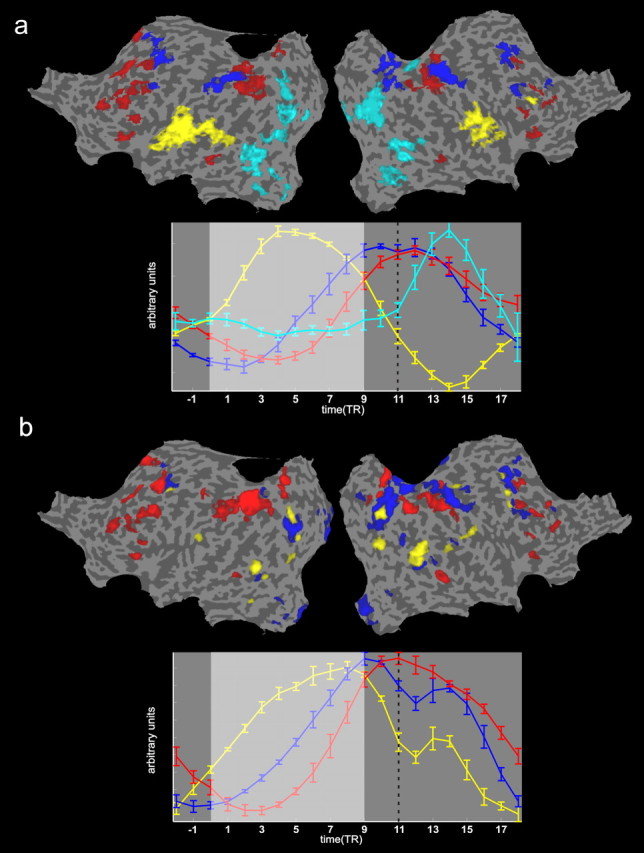
fMRI functional connectivity I (fuzzy clustering). Single-subject functional connectivity during task execution was examined by partitioning the cortical voxels into “clusters” of activation using fuzzy clustering (for details, see Materials and Methods). A, B, The single-subject results of all task-relevant clusters and their respective cluster time courses after averaging across all four functional runs, separately shown for the auditory (A) and visual (B) imagery conditions. Spatial maps are projected onto the flattened representation of the subject brain. For each cluster, the mean time course over the four runs of the centroid is presented in matched color in a respective time course graph below each map. Within both graphs showing the centroid time courses of these clusters (A, B, bottom), the light gray background shading represents the period within the experimental design during which the visual or auditory instructions were presented. The vertical black dotted line marks the time point at which the visual target stimulus was shown at the end of each trial. The error bars of each centroid time course represent the variance across the four functional runs of this single participant. Fuzzy clustering maps were thresholded corresponding to a threshold for a voxel membership at >0.5. Because the sum of the membership values for a voxel is 1, setting a 0.5 threshold corresponds to considering only those voxels that clearly belong to one cluster. The set of task-related clusters included a “sensory” cluster, accounting for the responses to the auditory or visual (depending on the experimental run) instructions (color code, yellow), two frontoparietal clusters, which we labeled, based on the relative timing of their time courses, “imagery early” (color code, blue) and “imagery late” (color code, red), and in case of the auditory condition, a second visual cluster that accounted for the response of the visual cortex to the presentation of the visual target (color code, cyan). Note that in the visual condition, this target-related response is represented by a second peak in the centroid time course of the sensory cluster (color code, yellow). For a full inspection of all clusters revealed by this analysis in this exemplary participant, see supplemental Figures S1–S4 (available at www.jneurosci.org as supplemental material).

Figure 5.

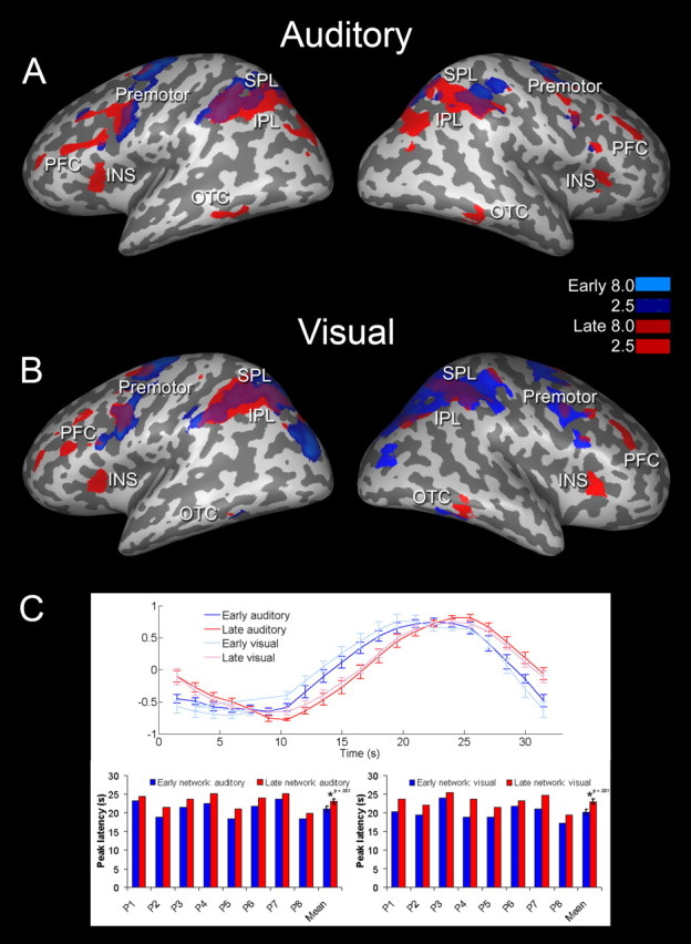
fMRI functional connectivity II (fuzzy clustering). A, B, Group multivariate functional connectivity maps, separately shown for the auditory (A) and visual (B) imagery conditions. This fuzzy clustering clearly separated an early (blue) from a late (red) bilateral frontoparietal activity cluster. C, Top, Standardized cluster time courses indicate similar functional roles of both imagery conditions during two distinct temporal stages (blue, early; red, late; light, visual; dark, auditory). C, Bottom, The temporal difference (peak latencies of BOLD signal) between the early (blue) and late (red) frontoparietal imagery network for all eight individual participants as well as for the group average. The mean temporal difference between the early and late frontoparietal imagery network was 2.8 s for the visual condition (t₍₇₎ = 6.9; p < 0.01) and 2.1 s for the auditory condition (t₍₇₎ = 9.7; p < 0.01). Each cluster is thus associated with a different temporal dynamic of activation. Fuzzy clustering maps were thresholded corresponding to a normalized mean score of 2.5 (see Materials and Methods). Data were projected on an inflated surface of an MNI template brain. IPL, Inferior parietal lobule; PFC, prefrontal cortex; INS, insular cortex.

Using such a data-driven multivariate approach has several appealing properties in the context of understanding the neural basis of complex cognitive tasks such as spatial imagery (see also Formisano and Goebel, 2003). First, the description of the sequence of spatial brain activation patterns is obtained blindly, i.e., without strong a priori assumptions about the temporal profile of the effects of interest or of the confounding factors. This reduces the problem of having an explicit model of the hemodynamic response, which may be problematic in the case of very different responses in different brain regions (see e.g., time courses in Fig. 3). Second, in contrast to the strictly location-based conventional (univariate) analyses, multivariate approaches highlight the involvement of spatially remote brain regions with covarying time courses in the same stage of the imagery task. Hence, by concurrently accounting for the full spatiotemporal pattern of brain activity including voxels with covarying hemodynamic time courses at spatially remote brain regions, the fuzzy clustering algorithm assesses the functional connectivity between all coactivated brain regions simultaneously across the entire brain.

Figure 3.

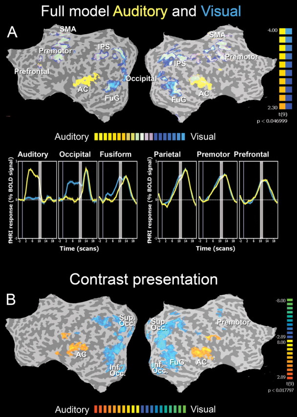
fMRI group GLM results. Random effects group fMRI results for both imagery conditions. A, Top, The overall GLM, revealing all significantly activated brain regions during the entire imagery trial, color coded separately for the visual (light to dark blue) and auditory (light to dark yellow) imagery conditions, superimposed on the same cortical flat map representation. A, Bottom, The BOLD signal time courses of six different significantly activated brain regions as seen in the spatial map above, separately shown for the visual (blue) and auditory (yellow) imagery conditions. The vertical gray bars within the BOLD signal time courses represent the presentation of the visual target stimulus at the end of each trial. B, The direct statistical contrast between the two imagery conditions during the stimulus presentation itself. During the visual condition, modality-specific BOLD signal increases were found in superior occipital and inferior parietal cortex (color coded in blue), whereas during the auditory condition significant higher activity changes were revealed in mainly auditory brain regions (color coded in orange). Group GLM maps were thresholded at a false discovery rate of q < 0.001. Results are superimposed on the flattened hemispheres of the MNI template brain. AC, Auditory cortex; Sup. Occ., superior occipital cortex; FuG, fusiform gyrus; IPS, intraparietal sulcus; SMA, supplementary motor area.

Effective brain connectivity (Granger causality).

Effective brain connectivity analyses were performed using Granger causality mapping (GCM). GCM is a technique that explores directed influences (effective connectivity) between distinct regions in fMRI data. GCM is computed with respect to a single selected reference region, and maps both sources of influence to the reference region and targets of influence from the reference region by making use of the concept of Granger causality to define what “influence” or “causality” means in the context of fMRI time series. A (discrete) time series X(t) is said to Granger cause a (discrete) time series Y(t) if the past of X improves the prediction of the current value of Y, given that all other relevant sources of influence (at the very least Y's own past) have been taken into account. Analogously, and independently, Granger causality from Y to X can be defined. Finally, instantaneous influence (correlation) between X and Y is said to exist when values X(t) improve predictions of contemporaneous values Y(t) (or vice versa, instantaneous correlation is symmetric), taking into account all other relevant sources of influence (at the very least the past of both X and Y). Temporal information in the data are used to define the existence and direction of influences without a directed graph model of assumed regional connections. These definitions can be applied to fMRI time series using vector autoregressive models (Roebroeck et al., 2005). The task-related directed influences were computed for every voxel between the average time course of the voxels in the selected reference regions and all other voxel time courses (multivariate) across the entire brain. Hence, for a given reference region, both sources of influence to the reference region (color code, green) and targets (color code, blue) of influence from the reference region (color code, red) are determined over the whole brain. All reference regions involved in either of the two imagery task were selected as seed regions for GCM. Importantly, both sources of influence to the reference region and targets of influence from the reference region were only considered as established when a subsequent selection of these suggested sources or targets revealed the initial reference as a new target or source region, respectively. This cross-validation analysis was done for all directed influences and allows the presented GCMs to be reciprocally interpreted (see Figs. 6, 7). Group GCM maps were thresholded at a false discovery rate of q < 0.05 as determined by bootstrapping of surrogate data. Empirical null distributions were obtained by (1) randomly selecting 1000 voxels, (2) estimating an autoregressive model of order = 2, (3) creating a simulated time series for each of these voxels, and (4) recomputing the bivariate Granger causality terms between the reference region of interest (ROI) and these simulated time series. Because influence from observations of the reference ROI to these surrogate data can only be attributable to chance, the resulting distribution of values can be used to estimate the null hypothesis of F_x→y − F_y→x = 0. Note that with this method for bootstrapping, simulated time series used for estimating the null hypothesis distribution preserve the temporal structure of the original time series. Finally, thresholding of the GCMs is based on false discovery rate, controlling for the multiple tests that are performed. For details on GCM, see Goebel et al. (2003) and Roebroeck et al. (2005). Granger causality maps were superimposed on the inflated representation of a template brain (MNI).

Figure 6.

fMRI effective brain connectivity for early imagery network. Group fMRI analyses of effective brain connectivity using GCM are shown. We used GCM for revealing both the sources of influence to a selected reference region (color coded in green) and the targets of influence from the respective reference region (color coded in blue) across the entire brain. These effective connectivity analyses explicitly tested for the causal influence one neural system exerts over another (see Materials and Methods). Group GCM maps were thresholded at a false discovery rate (FDR) of q < 0.05 as determined by bootstrapping of surrogate data (for details, see Materials and Methods). Areas color coded in green represent sources of influence to the reference region (red), and areas color coded in blue represent targets of influence from the reference region (red). GCMs are projected on inflated surfaces of an MNI template brain. A, These brain connectivity maps clearly revealed that early right premotor cortex sends neural input to bilateral SPL. B, This is cross-validated by having early left SPL as a reference region and revealing that although both parietal cortices receive neural input from source regions within bilateral premotor cortex, only the left parietal regions receive additional neural input from bilateral occipitoparietal and parietal source regions. In contrast, the same parietal regions in the right hemisphere mainly show neural target regions within bilateral parietal cortex. IPL, Inferior parietal lobule; Sup. Occ, superior occipital cortex.

Figure 7.

fMRI effective brain connectivity for late imagery network. Group fMRI analyses of effective brain connectivity using GCM. We used GCM for revealing both the sources of influence to a selected reference region (color coded in green) and the targets of influence from the respective reference region (color coded in blue) across the entire brain. These effective connectivity analyses explicitly tested for the causal influence one neural system exerts over another (see Materials and Methods). Group GCM maps were thresholded at a false discovery rate (FDR) of q < 0.05 as determined by bootstrapping of surrogate data. Areas color coded in green represent sources of influence to the reference region (red), and areas color coded in blue represent targets of influence from the reference region (red). GCMs are projected on inflated surfaces of an MNI template brain. A, Top and middle rows, These effective brain connectivity maps clearly revealed that the late right premotor cortex serves as a neural input to bilateral prefrontal and right OTC (A, top row), whereas the late left premotor cortex is characterized by projecting to bilateral OTC and, more importantly, by sending a second loop of neural input to extended parietal target regions within both hemispheres (A, middle row). A, Bottom row, From those bilateral parietal regions receiving input from late left premotor cortex, the left parietal areas in turn serve as neural input for bilateral OTC, while at the same time also receiving neural input from large bilateral frontoparietal source regions. B, In a last processing stage, both premotor cortices directly project to bilateral prefrontal areas as additional target regions. IPL, Inferior parietal lobule; PFC, prefrontal cortex; Sup. Occ., superior occipital cortex.

Results

Behavioral

The behavioral paradigm was designed to engage participants in the construction, maintenance, and spatial transformation of mental images generated from different input modalities (Fig. 1). The analyses of the behavioral data acquired inside the MR scanner focused on two questions: (1) do both input modalities (visual vs auditory) significantly differ in their behavioral responses? and (2) does the reaction time required to indicate whether target object and mentally constructed object are identical or not systematically increase with increasing rotational angle of the presented target object (angle distance effect)?

Before inference statistical testing, statistical outliers, defined as differing more than two SDs from the mean, were identified and removed from the behavioral dataset. For the reaction time data, only trials with correct responses were considered and averaged for the different experimental conditions. The reaction time data of the correct responses was further tested for normal distribution and variance homogeneity, confirming the suitability of the data for parametric statistical testing. Tests of significance were performed using a two-factorial repeated-measurement ANOVA with (1) input modality (two levels) and (2) rotational angle (three levels) as within-subject factors. Based on the results of this full factorial ANOVA, several simple post hoc contrast analyses were performed for each condition.

Input modality

The average reaction time (RT) required to perform the spatial imagery task and the respective level of accuracy were almost identical between the visual and auditory input modality (Fig. 2). Accordingly, input modality showed no significant main effect within the two-factorial ANOVA (RT, F_(1,9) = 3.094; p = 0.112; error, F_(1,9) = 0.053; p = 0.823).

Figure 2.

Behavioral results. Mean reaction times in milliseconds (plus SE) for performing the spatial imagery paradigm are separately shown for both imagery conditions and the three angular disparities. Data analyses were restricted to correct responses for nonmirrored targets. In both imagery conditions, reaction times significantly increased with increasing angular disparities. This angular distance effect traditionally has been interpreted as strong evidence for the actual use of mental imagery by the subjects. Please also note that the general difficulty level between both imagery conditions is identical, because no main effect of input modality, nor an interaction between input modality and angular disparity, was observed.

Stimulus rotation angle

Reaction times and error rates systematically increased with increasing angular disparities, from 1860 ms (1.5 errors) in the 40°-angle, to 2091 ms (2.5 errors) in the 80°-angle condition, to 2287 ms (3.1 errors) in the 120°-angle condition. Stimulus rotation angle showed a significant main effect within the two-factorial ANOVA (RT, F_(2,9) = 7.075; p < 0.05; error, F_(2,9) = 3.944; p < 0.05). This angle distance effect was independent from input modality as revealed by an absence of a significant interaction between input modality and rotational angle (RT, F_(2,9) = 1.003; p = 0.387; error, F_(2,9) = 0.612; p = 0.553) (Fig. 2).

Short summary behavioral data during fMRI

The behavioral data acquired during the fMRI experiment revealed that both visual and auditory input modality evoked the performance of spatial imagery with a respective rotational angle distance effect, i.e., increasing reaction times with increasing angular disparities. Moreover, the general difficulty level between both imagery conditions was statistically matched in terms of RT and accuracy.

fMRI

Conventional univariate analyses

The functional magnetic resonance imaging data were initially analyzed using conventional univariate multiple regression analysis.

These analyses revealed that during the execution of both task conditions, i.e., spatial imagery based on visual and auditory instructions, modality-specific sensory brain regions were activated, accompanied by a mutual largely distributed bilateral frontoparietal brain network (Fig. 3A). The spatial layout of this mental imagery network consisted of bilateral intraparietal sulcus, supplementary motor area, occipital cortex, inferior temporal cortex, prefrontal cortex, premotor cortex, and fusiform gyrus, and is in accordance with the results of several previous imaging studies investigating the neural correlates of spatial imagery (Kosslyn et al., 1993, 1998; Kawashima et al., 1995; Mellet et al., 1995, 1996, 1998, 2000b; Cohen et al., 1996; Tagaris et al., 1997; Carpenter et al., 1999; Richter et al., 2000; Trojano et al., 2000; Lamm et al., 2001; Formisano et al., 2002; Sack et al., 2002b, 2005). The modality-specific differences were mainly revealed in the auditory cortex (yellow indicates only active during auditory condition) and occipital regions/fusiform gyrus (light blue indicates only active during visual condition). The respective BOLD signal time courses of these regions further indicate that whereas auditory, occipital, and fusiform cortex show BOLD signal responses that are specific to the respective imagery condition, parietal, premotor, and prefrontal cortices are characterized by both a similar spatial layout (Fig. 3A, top) and identical BOLD signal time courses (Fig. 3A, bottom) between visual and auditory imagery.

Accordingly, when directly contrasting the visual and auditory predictors representing the different stages during the spatial imagery paradigm, the only significant activity differences between visual and auditory input modality were found during the presentation of the visual or auditory instructions, respectively. A contrast between the two input modalities revealed modality-specific BOLD signal increases within the respective sensory brain areas, with higher activity during visual stimulus presentation in superior occipital, fusiform gyrus, and inferior parietal cortex, and higher activity changes in auditory regions within temporal cortex during auditory stimulus presentation (Fig. 3B).

In a next step, we conducted functional and effective brain connectivity analyses, aiming to reveal the specific spatiotemporal dynamics within this large frontoparietal activation network and to perform a systematic analysis of both the similarities and differences in BOLD signal responses (Fig. 3A, bottom) related to the imagery task. We split up all functional runs into their respective visual and auditory trials, applied a multivariate data-driven fuzzy clustering algorithm separately to the auditory and visual imagery conditions, and subsequently conducted Granger causality mapping (for details, see Materials and Methods).

Fuzzy clustering

For both imagery conditions, fuzzy clustering consistently extracted several brain activity clusters with specific functional characteristics, each likely representing a distinct mental sub stage during the execution of the spatial imagery task. Concretely, the decomposition of the functional MRI time series with fuzzy clustering consistently produced (1) a set of imagery-related clusters (supplemental Figs. S1, S3, available at www.jneurosci.org as supplemental material), (2) a set of noise and artifact (e.g., motion) clusters (supplemental Figs. S2, S4, available at www.jneurosci.org as supplemental material), and (3) “default mode network” clusters (supplemental Figs. S1, S3, available at www.jneurosci.org as supplemental material).

Although a complete list of all revealed clusters is provided in the supplemental material (available at www.jneurosci.org), clusters differed in their ISC and thus in the consistency with which they were revealed across participants. However, because we were interested in those clusters that could be found with a certain consistency across participants, we followed the following formal criteria for cluster selection as presented in the main manuscript: (1) clusters had to be consistently revealed across participants with a minimum ISC of 85%, and (2) cluster centroid time courses had to positively correlate with the imagery paradigm. The latter was included because a detailed analysis and interpretation of, e.g., the default-mode-network clusters showing the typical map of negative signal changes during the task was beyond the scope of our study (although it is worth noting that our clustering algorithm consistently detected this network in all of the runs/subjects with an ISC of 100%) (see supplemental Figs. S1, S3, available at www.jneurosci.org as supplemental material).

Figure 4 depicts these consistent imagery-related clusters as revealed in an exemplary participant, and their respective cluster time courses in relation to the experimental imagery design, separately for the auditory (Fig. 4A) and visual (Fig. 4B) imagery conditions. This set of imagery-related clusters included one or two “sensory” clusters (color code, yellow), accounting for the responses to the auditory or visual (depending on the experimental run) instructions, two frontoparietal clusters, which we labeled, based on the relative timing of their time courses, “imagery early” (color code, blue) and “imagery late” (color code, red), and in the case of the auditory condition, a second visual cluster that accounted for the response of the visual cortex to the presentation of the visual target (color code, cyan; note that in the visual condition, this target-related response is represented by a second peak in the centroid time course of the sensory cluster). For a full inspection of all clusters revealed by this analysis in this exemplary participant, see supplemental Figures S1–S4 (available at www.jneurosci.org as supplemental material).

In terms of temporal sequence and direct relation to our experimental design, the first regions activated are thus mainly primary and secondary sensory brain areas as a direct consequence of the stimulus presentation in each imagery condition. This sensory encoding cluster represents the modality-specific stimulus processing stage within respective visual versus auditory sensory brain regions, and is temporarily directly related to the visual versus auditory input modality (yellow cluster and yellow centroid time course). In addition to this stimulus-driven activation cluster, we also identified a clear target-related cluster that occurs at the end of the trial, and that activates respective visual regions in the brain as a consequence of the presentation of the visual target stimulus (Fig. 4A, cyan cluster). Because for the visual condition, stimulus presentation (sensory encoding) and target are sharing the same modality, this target-related response is represented by a second peak in the extracted sensory cluster (Fig. 4B, yellow cluster).

Cognitively more interestingly are, however, the modality-independent clusters that are neither directly stimulus nor target related, but that rather show task-relevant activation in between these two stages. These clusters are likely to represent different cognitive mental subprocesses associated with spatial imagery such as image construction, maintenance, or spatial transformation (Fig. 4, blue and red clusters). The fact that these two premotor–parietal clusters show cluster centroids (i.e., time courses) clearly compatible with the activations of these regions during the construction of the mental image/maintenance stage of our task (i.e., they are neither directly stimulus-onset, nor target or motor related) and the fact that we revealed these two distinct imagery networks in each functional run of each participant support the notion that both imagery conditions, visual and auditory, are separated into two distinct frontoparietal networks with distinct spatial layout, temporal dynamics, and functional characteristics.

When averaging single-subject cluster maps after normalization to Talairach space, we functionally separated an early (blue) from a late (red) bilateral frontoparietal activity cluster also on a group level (Fig. 5A,B).

A quantitative analysis of the underlying BOLD peak latencies revealed that the late frontoparietal activity cluster was activated 2.1 s after the early frontoparietal cluster during the auditory condition and 2.8 s after the early frontoparietal cluster during the visual condition. These quantified temporal dynamics thus revealed a consistent latency difference between the early and late frontoparietal activity network (Fig. 5C). Please note that this temporal difference between early and late frontoparietal activation was consistently found in all eight participants (Table 1), and proved to be statistically significant (auditory condition, t₍₇₎ = 9.7; p < 0.01; visual condition, t₍₇₎ = 6.9; p < 0.01).

Table 1.

Peak latencies (in seconds) of BOLD signal changes during auditory and visual imagery conditions, separately shown for all eight participants (P1–P8) and the early versus late frontoparietal network

Frontoparietal network	Participants								Statistics
	P1	P2	P3	P4	P5	P6	P7	P8	Mean	SEM	t(7)	p
Auditory
Early	23.3	18.8	21.4	22.5	18.4	21.8	23.6	18.4	21.0	0.776
Late	24.4	21.4	23.6	25.1	21.0	24.0	25.1	19.9	23.1	0.716
Difference	1.1	2.6	2.3	2.6	2.6	2.3	1.5	1.5	2.1		9.701	0.000
Visual
Early	20.3	19.5	24.0	18.8	18.8	21.8	21.0	17.2	20.2	0.742
Late	23.6	22.1	25.5	23.6	21.4	23.3	24.8	19.5	23.0	0.679
Difference	3.4	2.6	1.5	4.8	2.6	1.5	3.8	2.3	2.8		6.908	0.000

In terms of spatial layout, the group clustering maps (Fig. 5) reveal some overlap between the early and late imagery network as a consequence of averaging cluster maps across subjects. However, there were also consistent differences. For the auditory condition, the earlier cluster included mainly lateral SPL and premotor regions, whereas the late cluster was characterized more by inferior parietal areas, prefrontal cortex, and anterior occipitotemporal cortex (OTC). In the visual imagery condition, the earlier cluster included inferior parietal regions, premotor regions, and posterior OTC, whereas the late cluster was characterized by lateral SPL, prefrontal cortex, and anterior OTC. Interestingly, for both imagery conditions, only the late parietal cluster seemed to simultaneously recruit extended bilateral prefrontal regions, whereas the early parietal cluster involved more premotor regions (Fig. 5). To also quantify and statistically analyze this difference in spatial layout between the early and late frontoparietal activity network, we quantified both the direction and magnitude of the exact shift in spatial coordinates between the parietal contributions within the early versus late imagery cluster by calculating the subject-specific euclidean distance between the respective cluster activation peaks. These analyses revealed that during the auditory imagery condition, the average euclidean distance between the early and late parietal activity cluster was 23.8 mm (SD = 9.5) and 20.2 mm (SD = 9.9) in lateral-ventral-inferior direction for the left and right hemispheres, respectively. For the visual imagery condition, euclidean distances between early and late parietal activity cluster were 21.7 mm (SD = 11.4) and 29.5 mm (SD = 16.6) in lateral-ventral-inferior direction for the left and right hemispheres, respectively. This quantified difference in spatial layout between early and late parietal activation was consistently found in all eight participants (Table 2), and proved to be statistically significant (auditory condition left parietal, t₍₇₎ = 7.1; p < 0.01; auditory condition right parietal, t₍₇₎ = 5.8; p < 0.01; visual condition left parietal, t₍₇₎ = 5.4; p < 0.01; visual condition right parietal, t₍₇₎ = 5.4; p < 0.01).

Table 2.

Euclidean distance (in millimeters) in lateral-ventral-inferior direction between early and late imagery network, separately shown for all eight participants (P1–P8) and left versus right hemisphere

Condition	Participants								Statistics
	P1	P2	P3	P4	P5	P6	P7	P8	Mean	SD	t(7)	p
Auditory
LH	30.9	18.8	30.0	34.8	23.0	11.6	9.9	31.4	23.8	9.5	7.077	0.0002
RH	18.8	31.4	13.7	38.1	15.3	22.0	9.4	13.2	20.2	9.9	5.788	0.0006
Visual
LH	21.4	17.8	41.7	7.8	13.2	15.1	21.8	35	21.7	11.4	5.412	0.001
RH	17.2	28.1	19.8	54.2	36.3	14.3	16.6	49.6	29.5	15.6	5.353	0.001

LH, Left hemisphere; RH, right hemisphere.

Moreover, we also identified specific differences in the functional connectivity maps between the visual versus auditory imagery condition (Fig. 5). One of the most interesting differences between visual and auditory spatial imagery was represented by the modality-specific involvement of the OTC. When comparing both imagery conditions, we found OTC activation within the early frontoparietal cluster only for the visual but not for auditory condition. However, during the late frontoparietal activity cluster both imagery conditions, auditory and visual, coactivated bilateral OTC (Fig. 5). Hence, also the OTC can be functionally segregated into an early and late component, with the visual condition including both early and late OTC activity, and the auditory condition exclusively including the late OTC component. In terms of spatial layout, the late OTC component was located adjacent but anterior with respect to the early OTC activation (Fig. 5).

Effective brain connectivity

In a further step, we also applied effective brain connectivity analyses and defined the existence and direction of neural influences between the revealed functionally connected brain regions. More specifically, we used GCM (Roebroeck et al., 2005) for revealing both the sources of influence to a selected reference region, as well as the targets of influence from the respective reference region across the entire brain. In contrast to the above-described functional connectivity analyses, these effective connectivity analyses explicitly tested for the causal influence one neural system exerts over another (Friston, 1993). In this sense, Granger causality mapping provides information regarding the direction of neural information processing within a distributed brain network in which activity in one brain area might Granger cause activity in another brain region. Importantly, all calculated directed influences between brain regions underwent a systematic cross-validation analysis and are thus reciprocally interpretational. In other words, a brain region showing up as, e.g., a source region for a given reference region, will in turn reveal this region as a target when being selected as a new reference (for details, see Materials and Methods).

In an attempt to track the causal direction of the entire flow of neural information during both imagery conditions, we started seeding GCM reference regions within both sensory cortices. However, although during the sensory input stage both imagery conditions show modality-specific instantaneous correlations between the respective sensory cortex and bilateral premotor–parietal networks, a clear direction of neural information flow from or to specific regions within these networks could not be resolved because this connectivity was bidirectional in nature and occurred on a time scale outside the functional resolution of Granger causality mapping (Roebroeck et al. (2005).

However, although the question of directivity between sensory and premotor–parietal cortex connectivity remains open, we were able to reveal that the neuronal activities associated with both imagery conditions already converge at the stage of the identified early premotor–parietal connectivity loop. During this early and modality-independent mental imagery network, bilateral premotor regions send neural activity to left and right parietal cortex as their target regions (Fig. 6A,B, dotted blue arrows). Interestingly, from those bilateral parietal regions receiving input from early right premotor cortex, only the left parietal regions receive additional neural input from bilateral occipitoparietal and parietal source regions, whereas the same parietal regions in the right hemisphere mainly show neural target regions within bilateral parietal cortex (Fig. 6B, solid blue arrows).

During the late modality-independent mental imagery network, bilateral premotor cortex shows an effective connectivity to OTC that is absent during the early frontoparietal cluster (Fig. 7A, top and middle rows, red arrows). Interestingly, the late left premotor cortex projects to bilateral OTC (Fig. 7A, middle row, dotted red arrows), whereas late right premotor cortex serves as a neural input exclusively to ipsilateral OTC (Fig. 7A, top row, solid red arrows). At the same time, whereas late right premotor cortex shows no effective connectivity to parietal cortex (Fig. 7A, top row), late left premotor cortex is characterized by sending neural input to extended parietal target regions within both hemispheres (Fig. 7A, middle row, dotted red arrows). In fact, for the right premotor cortex, the late right premotor activity component projects only to bilateral prefrontal and right OTC but no parietal regions (Fig. 7A, top row, solid red arrows), whereas the early right premotor activity component projects only to bilateral parietal but no prefrontal regions (Fig. 6B, dotted blue arrows). From those bilateral parietal regions receiving input from late left premotor cortex, the right parietal areas project to right OTC target regions, whereas the left parietal areas in turn serve as neural input for bilateral OTC (Fig. 7A, middle and bottom rows). Also, this late left parietal area seem to in turn receive neural feedback from the posterior part of left and right OTC, suggesting a possible feedback from OTC to parietal cortex during this late premotor–parietal–OTC cluster (Fig. 7A, bottom row). Interestingly, we revealed that only during the auditory imagery condition, these late left parietal activities at the same time receive neural input from large bilateral frontoparietal brain regions (Fig. 7A, bottom row, solid red arrow), whereas during visual imagery, the late parietal cortices mainly project to prefrontal target regions.

Finally, after this late premotor–parietal–OTC imagery network, a last processing stage occurred during which both premotor cortices directly project to bilateral prefrontal areas as additional target regions (Fig. 7B, dotted purple arrows).

Discussion

Angle distance effect

Both imagery conditions showed a linear correlation between performance and required angle of mental rotation. This angular distance effect has been interpreted as evidence for the actual use of mental imagery: if an increment of time is required for each degree of angular disparity, participants can be assumed to perform such tasks by “mentally rotating” an object as if it were moving through the intermediate positions along a trajectory (Kosslyn et al., 1998; Palmer, 1999; Vingerhoets et al., 2002).

Two distinct frontoparietal imagery networks

Our analyses revealed that both imagery conditions converge in similar brain networks comprised of bilateral parietal, prefrontal, premotor, and OTC activity changes. However, our analytical framework enabled us to reveal that this general bilateral frontoparietal activity can be functionally segregated into two distinct frontoparietal–OTC imagery networks. We functionally segregated an early from a late bilateral parietal activation cluster, which was orchestrated by respective early versus late premotor, OTC, and late prefrontal activity changes. In addition to being involved at two clearly separable temporal stages during spatial imagery, the early versus late imagery network also differ in spatial layout. Whereas the late parietal imagery cluster was orchestrated by simultaneously recruited bilateral prefrontal regions, the early parietal imagery cluster involved more premotor regions.

Interestingly, whereas the premotor and prefrontal contributions within these two imagery clusters remained consistent in terms of spatial layout and assignment to the early versus late frontoparietal cluster between both imagery conditions, the parietal contributions seem to shift in spatial coordinates between visual versus auditory imagery. For the auditory condition, the earlier imagery cluster included mainly lateral SPL and the late cluster more inferior parietal areas, whereas in the visual imagery condition the earlier cluster included inferior parietal regions and the late cluster more lateral SPL. We interpret this difference in spatial layout between both conditions with regard to the imagery task during which the construction phase of the mental image and the processing of the sequentially presented verbal versus visual instructions were interspersed. In case of the visual imagery condition, the online construction of the mental object was mediated by inferior parietal regions and thus bottom-up from the visual to the inferior parietal cortex, whereas at the same stage during the auditory condition, the sequentially presented verbal instructions were processed within primary and secondary auditory cortex and mediated via the temporoparietal junction to lateral SPL regions.

In this context of modality-specific differences, we could also functionally segregate the OTC into an early posterior versus late anterior activation cluster. This association of the ventral pathway with visual object or visual shape imagery has been shown in a variety of other studies on mental imagery (Kosslyn et al., 1993; Roland and Gulyas, 1995; Mellet et al., 1996; D'Esposito et al., 1997; Mellet et al., 1998) and suggests the specific involvement of this region for object shape processing both in visual perception and in visual imagery (Ishai et al., 2000). Interestingly, the visual imagery condition involved early and late OTC activity, whereas the auditory imagery condition only included late OTC activity. The early OTC cluster might thus represent the online assembling of the sequentially presented visual information into one final slowly emerging visual object, whereas the late OTC could represent the pure object imagery counterpart of a mental object that is merely constructed from verbal descriptions and that has thus never been perceptually encountered before. Further support for this interpretation comes from the conducted effective connectivity analyses, which revealed that the neural input for the late OTC cluster (pure object imagery) comes from late premotor and parietal cortex, i.e., top-down from higher motor-perceptual brain regions, whereas the early OTC activity (slowly emerging visual object) receives its neural input from superior occipital brain regions, thus bottom-up from the visual system. Interestingly, we also revealed that the late OTC cluster not only received neural input from late parietal cortex, but that the posterior part of this late OTC region in turn sent information back to parietal cortex, suggesting a possible dynamic feedback loop between parietal cortex and OTC during the late premotor–parietal activation cluster.

Dynamics within imagery networks

On a more general level, our findings demonstrate that the execution of visuospatial tasks based on both visual stimuli (Haxby et al., 1991; Ungerleider and Haxby, 1994; Cohen et al., 1996; Goebel et al., 1998; Trojano et al., 2000; Sack et al., 2002a) and mentally constructed stimuli (Mellet et al., 1996; Trojano et al., 2000; Sack et al., 2002b) leads to increased activations in the frontoparietal cortices of the human brain. In addition, the applied brain network effective connectivity analyses revealed a complex but integrated picture of recurrent information flow within the revealed frontoparietal–OTC networks. The information upcoming from modality-specific sensory brain regions is first sent to the premotor cortex and then to the medial dorsal parietal cortex, indicating that the activation flow processes the construction and spatial transformation of visual mental images in a top-down manner from the motor to the perceptual pole of spatial imagery. Importantly, the premotor cortex moreover plays the crucial role of a central relay station projecting to parietal cortex at two functionally distinct temporal stages during spatial imagery with the late premotor activity cluster showing a left-lateralized second feedback loop to lateral ventral parietal cortex. During this late premotor–parietal activity cluster, neural input is also sent from the premotor cortex to bilateral prefrontal and OTC regions.

Based on our findings, we propose that the described sequence of dynamic premotor-to-parietal interactions subserve different cognitive subprocesses associated with spatial imagery (Fig. 8).

Figure 8.

Dynamic premotor–parietal interactions during spatial imagery. All applied analyses are integrated into one dynamic model of multisensory spatial imagery. Each color depicts a separate connectivity network underlying a distinct cognitive (sub)function. The arrows correspond to the causal influence one neural system exerts over another neural system and are thus indicative of the directed influence of information flow within these networks. Dotted lines represent connectivity to bilateral target sites, whereas solid lines indicate projections to unilateral target sites only. We could reveal that the modality-specific neural activity changes within the respective sensory brain regions show instantaneous correlations to large bilateral premotor–parietal networks whose directivity could not be resolved with GCM (nondirectional dotted yellow lines). However, within this early premotor–parietal network, both premotor cortices project to bilateral parietal cortex (blue), thereby constituting the early frontoparietal activity network. In contrast, the late premotor cortex activity shows a clear hemispheric lateralization with only the late left premotor cortex projecting a second feedback loop to bilateral parietal cortex and bilateral OTC (red dotted), whereas the late right premotor cortex projects only to right OTC (red solid). Finally, bilateral late premotor cortex also projects to bilateral prefrontal cortex (purple). The temporal order of these distinct brain networks represents distinct cognitive subprocesses including the following: (1) yellow, convergence from modality-dependent sensory pathways to modality-independent frontoparietal network; (2) blue, online processing of sequentially presented modality-independent spatial instructions; (3) red, construction of stepwise emerging final mental object and spatial analysis of the imagined content; and (4) purple, maintenance of spatially rotated final mental object in short-term memory and preparation of motor response. AC, Auditory cortex; Occ., occipital.

Multisensory imagery network

During the stimulus presentation stage, both imagery conditions (visual and auditory) show modality-specific sensory neural activity changes. Subsequently, the neuronal activities associated with both imagery conditions converge already at the stage of the identified early premotor–parietal activation cluster (Mellet et al., 1996, 1998, 2000a; Trojano et al., 2000).

Online processing of spatial information

Within this early premotor–parietal brain network, bilateral premotor activity projects to bilateral parietal brain regions. One might thus speculate that this early bilateral premotor–parietal activation network underlies the online processing of the sequentially presented modality-independent spatial instructions (Corbetta et al., 1993; Jonides et al., 1993; Haxby et al., 1994; Courtney et al., 1996).

Construction of an emerging mental object

In contrast, the late premotor–parietal activation cluster shows a left hemispheric lateralization because only the left late premotor cortex projects to late parietal brain regions. Importantly, this late left premotor–parietal activation network further sends neural signals to bilateral OTC. This specific effective connectivity network might thus represent the juxtaposing of the sequentially presented stimuli and thus the successive construction of the slowly emerging final mental object during imagery (Kosslyn et al., 1993; Roland and Gulyas, 1995; Mellet et al., 1996, 1998; D'Esposito et al., 1997).

Division of labor between hemispheres

This late parietal activation cluster receiving input from late left premotor cortex is characterized by strong bilateral parietal interactions within which left and right parietal cortex receive additional neural input from bilateral superior and inferior parietal brain regions. This late bilateral parietal activity might thus subserve the required spatial rotation of the constructed mental image, with the left hemisphere underlying construction and maintenance of the final mental image and the right hemisphere contributing to the required spatial analysis of the imagined content (Formisano et al., 2002; Sack et al., 2002b, 2005).

Short-term storage of constructed image

Finally, the late bilateral premotor–prefrontal activation network might subserve the necessary maintenance of the spatially rotated final visual mental object in short-term working memory for the required subsequent comparison with the presented visual target (Tulving et al., 1994; Moscovitch et al., 1995; Roland and Gulyas, 1995; Smith et al., 1995; Buckner et al., 1996; Cohen et al., 1997; Courtney et al., 1997).

However, some words of caution are required. First, despite the elaborated data-driven and multivariate analysis approaches conducted in this study, the interpretation of their specific functional contribution and thus the given cognitive labels for the revealed distinct activation clusters and effective brain connectivity networks are bound to remain speculative. Moreover, it needs to be noted that any interpretation regarding a potential temporal sequence of neural events based on BOLD fMRI signal analyses may always be confounded by potential hemodynamic response differences across brain regions. Nonetheless, the proposed sequence of effective connectivity networks described in our study is in agreement with several lines of research describing coupled activations of the parietal and premotor cortices during spatial localization (Haxby et al., 1994) or shifting of spatial attention (Corbetta et al., 1993), and in situations explicitly involving the spatial working memory (Jonides et al., 1993; Courtney et al., 1996). The exchange of information between the premotor regions and the dorsal route thus appears to be a general feature during spatial processing, whatever the nature of the initial input. Moreover, the perceptual parietal pole itself can be subdivided into at least two functionally distinct networks, an early premotor–parietal versus a late premotor–parietal imagery component. Interestingly, only the latter bilateral parietal activity shows an interhemispheric division of labor with the left parietal cortex underlying the generation of mental images and the right parietal cortex subserving the respective spatial analyses (Sack et al., 2005). On a methodological level, our findings demonstrate how regions that are conventionally modeled as functional units during fMRI are segregated into distinct subdivisions with different functional contributions. Our results highlight the importance of not only considering task-related activation levels at specific spatial locations, but systematically comparing the temporal dynamics of brain activities within and across brain areas when investigating the neurobiology of multifaceted cognitive functions.

References

- Bezdek JC, Ehrlich R, Full W. FCM: the fuzzy C-means clustering algorithm. Comput Geosci. 1984;10:191–203. [Google Scholar]
- Boynton GM, Engel SA, Glover GH, Heeger DJ. Linear systems analysis of functional magnetic resonance imaging in human V1. J Neurosci. 1996;16:4207–4221. doi: 10.1523/JNEUROSCI.16-13-04207.1996. [DOI] [PMC free article] [PubMed] [Google Scholar]
- Buckner RL, Raichle ME, Miezin FM, Petersen SE. Functional anatomic studies of memory retrieval for auditory words and visual pictures. J Neurosci. 1996;16:6219–6235. doi: 10.1523/JNEUROSCI.16-19-06219.1996. [DOI] [PMC free article] [PubMed] [Google Scholar]
- Carpenter PA, Just MA, Keller TA, Eddy W, Thulborn K. Graded functional activation in the visuospatial system with the amount of task demand. J Cogn Neurosci. 1999;11:9–24. doi: 10.1162/089892999563210. [DOI] [PubMed] [Google Scholar]
- Cohen JD, Perlstein WM, Braver TS, Nystrom LE, Noll DC, Jonides J, Smith EE. Temporal dynamics of brain activation during a working memory task. Nature. 1997;386:604–608. doi: 10.1038/386604a0. [DOI] [PubMed] [Google Scholar]
- Cohen MS, Kosslyn SM, Breiter HC, DiGirolamo GJ, Thompson WL, Anderson AK, Brookheimer SY, Rosen BR, Belliveau JW. Changes in cortical activity during mental rotation. A mapping study using functional MRI. Brain. 1996;119:89–100. doi: 10.1093/brain/119.1.89. [DOI] [PubMed] [Google Scholar]
- Corbetta M, Miezin FM, Shulman GL, Petersen SE. A PET study of visuospatial attention. J Neurosci. 1993;13:1202–1226. doi: 10.1523/JNEUROSCI.13-03-01202.1993. [DOI] [PMC free article] [PubMed] [Google Scholar]
- Courtney SM, Ungerleider LG, Keil K, Haxby JV. Object and spatial visual working memory activate separate neural systems in human cortex. Cereb Cortex. 1996;6:39–49. doi: 10.1093/cercor/6.1.39. [DOI] [PubMed] [Google Scholar]
- Courtney SM, Ungerleider LG, Keil K, Haxby JV. Transient and sustained activity in a distributed neural system for human working memory. Nature. 1997;386:608–611. doi: 10.1038/386608a0. [DOI] [PubMed] [Google Scholar]
- D'Esposito M, Detre JA, Aguirre GK, Stallcup M, Alsop DC, Tippet LJ, Farah MJ. A functional MRI study of mental image generation. Neuropsychologia. 1997;35:725–730. doi: 10.1016/s0028-3932(96)00121-2. [DOI] [PubMed] [Google Scholar]
- Formisano E, Goebel R. Tracking cognitive processes with functional MRI mental chronometry. Curr Opin Neurobiol. 2003;13:174–181. doi: 10.1016/s0959-4388(03)00044-8. [DOI] [PubMed] [Google Scholar]
- Formisano E, Linden DE, Di Salle F, Trojano L, Esposito F, Sack AT, Grossi D, Zanella FE, Goebel R. Tracking the mind's image in the brain I: time-resolved fMRI during visuospatial mental imagery. Neuron. 2002;35:185–194. doi: 10.1016/s0896-6273(02)00747-x. [DOI] [PubMed] [Google Scholar]
- Friston KJ. Characterizing focal and distributed physiological changes with neuroimaging. In: Uemura NA, Lassen NA, Jones T, Kanno I, editors. Quantification of brain function: tracer kinetics and image analysis in brain PET. New York: Elsevier Science; 1993. [Google Scholar]
- Friston KJ, Holmes AP, Poline JB, Grasby PJ, Williams SC, Frackowiak RS, Turner R. Analysis of fMRI time-series revisited. Neuroimage. 1995;2:45–53. doi: 10.1006/nimg.1995.1007. [DOI] [PubMed] [Google Scholar]
- Genovese CR, Lazar NA, Nichols T. Thresholding of statistical maps in functional neuroimaging using the false discovery rate. Neuroimage. 2002;15:870–878. doi: 10.1006/nimg.2001.1037. [DOI] [PubMed] [Google Scholar]
- Goebel R, Linden DE, Lanfermann H, Zanella FE, Singer W. Functional imaging of mirror and inverse reading reveals separate coactivated networks for oculomotion and spatial transformations. Neuroreport. 1998;9:713–719. doi: 10.1097/00001756-199803090-00028. [DOI] [PubMed] [Google Scholar]
- Goebel R, Roebroeck A, Kim DS, Formisano E. Investigating directed cortical interactions in time-resolved fMRI data using vector autoregressive modeling and Granger causality mapping. Magn Reson Imaging. 2003;21:1251–1261. doi: 10.1016/j.mri.2003.08.026. [DOI] [PubMed] [Google Scholar]
- Haxby JV, Grady CL, Horwitz B, Ungerleider LG, Mishkin M, Carson RE, Herscovitch P, Schapiro MB, Rapoport SI. Dissociation of object and spatial visual processing pathways in human extrastriate cortex. Proc Natl Acad Sci U S A. 1991;88:1621–1625. doi: 10.1073/pnas.88.5.1621. [DOI] [PMC free article] [PubMed] [Google Scholar]
- Haxby JV, Horwitz B, Ungerleider LG, Maisog JM, Pietrini P, Grady CL. The functional organization of human extrastriate cortex: a PET-rCBF study of selective attention to faces and locations. J Neurosci. 1994;14:6336–6353. doi: 10.1523/JNEUROSCI.14-11-06336.1994. [DOI] [PMC free article] [PubMed] [Google Scholar]
- Ishai A, Ungerleider LG, Haxby JV. Distributed neural systems for the generation of visual images. Neuron. 2000;28:979–990. doi: 10.1016/s0896-6273(00)00168-9. [DOI] [PubMed] [Google Scholar]
- Jonides J, Smith EE, Koeppe RA, Awh E, Minoshima S, Mintun MA. Spatial working memory in humans as revealed by PET. Nature. 1993;363:623–625. doi: 10.1038/363623a0. [DOI] [PubMed] [Google Scholar]
- Kawashima R, O'Sullivan BT, Roland PE. Positron-emission tomography studies of cross-modality inhibition in selective attentional tasks: closing the “mind's eye.”. Proc Natl Acad Sci U S A. 1995;92:5969–5972. doi: 10.1073/pnas.92.13.5969. [DOI] [PMC free article] [PubMed] [Google Scholar]
- Knauff M, Kassubek J, Mulack T, Greenlee MW. Cortical activation evoked by visual mental imagery as measured by fMRI. Neuroreport. 2000;11:3957–3962. doi: 10.1097/00001756-200012180-00011. [DOI] [PubMed] [Google Scholar]
- Kosslyn SM, Alpert NM, Thompson WL, Maljkovik V, Weise SB, Chabris CF, Hamilton SE, Rauch SL, Buonanno FS. Visual mental imagery activates topographically organized visual cortex: PET investigations. J Cogn Neurosci. 1993;5:263–287. doi: 10.1162/jocn.1993.5.3.263. [DOI] [PubMed] [Google Scholar]
- Kosslyn SM, DiGirolamo GJ, Thompson WL, Alpert NM. Mental rotation of objects versus hands: neural mechanisms revealed by positron emission tomography. Psychophysiology. 1998;35:151–161. [PubMed] [Google Scholar]
- Kosslyn SM, Ganis G, Thompson WL. Neural foundations of imagery. Nat Rev Neurosci. 2001;2:635–642. doi: 10.1038/35090055. [DOI] [PubMed] [Google Scholar]
- Lamm C, Windischberger C, Leodolter U, Moser E, Bauer H. Evidence for premotor cortex activity during dynamic visuospatial imagery from single-trial functional magnetic resonance imaging and event-related slow cortical potentials. Neuroimage. 2001;14:268–283. doi: 10.1006/nimg.2001.0850. [DOI] [PubMed] [Google Scholar]
- Mechelli A, Price CJ, Friston KJ, Ishai A. Where bottom-up meets top-down: neuronal interactions during perception and imagery. Cereb Cortex. 2004;14:1256–1265. doi: 10.1093/cercor/bhh087. [DOI] [PubMed] [Google Scholar]
- Mellet E, Tzourio N, Denis M, Mazoyer B. A positron emission tomography study of visual and mental spatial exploration. J Cogn Neurosci. 1995;7:433–445. doi: 10.1162/jocn.1995.7.4.433. [DOI] [PubMed] [Google Scholar]
- Mellet E, Tzourio N, Crivello F, Joliot M, Denis M, Mazoyer B. Functional anatomy of spatial mental imagery generated from verbal instructions. J Neurosci. 1996;16:6504–6512. doi: 10.1523/JNEUROSCI.16-20-06504.1996. [DOI] [PMC free article] [PubMed] [Google Scholar]
- Mellet E, Petit L, Mazoyer B, Denis M, Tzourio N. Reopening the mental imagery debate: lessons from functional anatomy. Neuroimage. 1998;8:129–139. doi: 10.1006/nimg.1998.0355. [DOI] [PubMed] [Google Scholar]
- Mellet E, Tzourio-Mazoyer N, Bricogne S, Mazoyer B, Kosslyn SM, Denis M. Functional anatomy of high-resolution visual mental imagery. J Cogn Neurosci. 2000a;12:98–109. doi: 10.1162/08989290051137620. [DOI] [PubMed] [Google Scholar]
- Mellet E, Briscogne S, Tzourio-Mazoyer N, Ghaëm O, Petit L, Zago L, Etard O, Berthoz A, Mazoyer B, Denis M. Neural correlates of topographic mental exploration: the impact of route versus survey perspective learning. Neuroimage. 2000b;12:588–600. doi: 10.1006/nimg.2000.0648. [DOI] [PubMed] [Google Scholar]
- Moscovitch C, Kapur S, Köhler S, Houle S. Distinct neural correlates of visual long-term memory for spatial location and object identity: a positron emission tomography study in humans. Proc Natl Acad Sci U S A. 1995;92:3721–3725. doi: 10.1073/pnas.92.9.3721. [DOI] [PMC free article] [PubMed] [Google Scholar]
- Palmer SE. Cambridge, MA: MIT; 1999. Vision science: photons to phenomenology. [Google Scholar]
- Richter W, Ugurbil K, Georgopoulos A, Kim SG. Time-resolved fMRI of mental rotation. Neuroreport. 1997;8:3697–3702. doi: 10.1097/00001756-199712010-00008. [DOI] [PubMed] [Google Scholar]
- Richter W, Somorjai R, Summers R, Jarmasz M, Menon RS, Gati JS, Georgopoulos AP, Tegeler C, Ugurbil K, Kim SG. Motor area activity during mental rotation studied by time-resolved single-trial fMRI. J Cogn Neurosci. 2000;12:310–320. doi: 10.1162/089892900562129. [DOI] [PubMed] [Google Scholar]
- Roebroeck A, Formisano E, Goebel R. Mapping directed influence over the brain using Granger causality and fMRI. Neuroimage. 2005;25:230–242. doi: 10.1016/j.neuroimage.2004.11.017. [DOI] [PubMed] [Google Scholar]
- Roland PE, Gulyás B. Visual memory, visual imagery, and visual recognition of large field patterns by the human brain: functional anatomy by positron emission tomography. Cereb Cortex. 1995;5:79–93. doi: 10.1093/cercor/5.1.79. [DOI] [PubMed] [Google Scholar]
- Sack AT, Hubl D, Prvulovic D, Formisano E, Jandl M, Zanella FE, Maurer K, Goebel R, Dierks T, Linden DE. The experimental combination of rTMS and fMRI reveals the functional relevance of parietal cortex for visuospatial functions. Brain Res Cogn Brain Res. 2002a;13:85–93. doi: 10.1016/s0926-6410(01)00087-8. [DOI] [PubMed] [Google Scholar]
- Sack AT, Sperling JM, Prvulovic D, Formisano E, Goebel R, Di Salle F, Dierks T, Linden DE, Formisano E, Linden DE, Di Salle F, Trojano L, Esposito F, Sack AT, Grossi D, Zanella FE, Goebel R. Tracking the mind's image in the brain II: transcranial magnetic stimulation reveals parietal asymmetry in visuospatial imagery. Neuron. 2002b;35:195–204. doi: 10.1016/s0896-6273(02)00745-6. [DOI] [PubMed] [Google Scholar]
- Sack AT, Camprodon JA, Pascual-Leone A, Goebel R. The dynamics of interhemispheric compensatory processes in mental imagery. Science. 2005;308:702–704. doi: 10.1126/science.1107784. [DOI] [PubMed] [Google Scholar]
- Smith EE, Jonides J, Koeppe RA, Awh E, Schumacher EH, Minoshima S. Spatial vs. object working memory: PET investigations. J Cogn Neurosci. 1995;7:337–356. doi: 10.1162/jocn.1995.7.3.337. [DOI] [PubMed] [Google Scholar]
- Smolders A, De Martino F, Staeren N, Scheunders P, Sijbers J, Goebel R, Formisano E. Dissecting cognitive stages with time-resolved fMRI data: a comparison of fuzzy clustering and independent component analysis. Magn Reson Imaging. 2007;25:860–868. doi: 10.1016/j.mri.2007.02.018. [DOI] [PubMed] [Google Scholar]
- Tagaris GA, Kim SG, Strupp JP, Andersen P, Ugurbil K, Georgopoulos AP. Mental rotation studied by functional magnetic resonance imaging at high field (4 Tesla): performance and cortical activation. J Cogn Neurosci. 1997;9:419–432. doi: 10.1162/jocn.1997.9.4.419. [DOI] [PubMed] [Google Scholar]
- Trojano L, Grossi D, Linden DE, Formisano E, Hacker H, Zanella FE, Goebel R, Di Salle F. Matching two imagined clocks: the functional anatomy of spatial analysis in the absence of visual stimulation. Cereb Cortex. 2000;10:473–481. doi: 10.1093/cercor/10.5.473. [DOI] [PubMed] [Google Scholar]
- Trojano L, Grossi D, Linden DE, Formisano E, Goebel R, Cirillo S, Elefante R, Di Salle F. Coordinate and categorical judgements in spatial imagery. An fMRI study. Neuropsychologia. 2002;40:1666–1674. doi: 10.1016/s0028-3932(02)00021-0. [DOI] [PubMed] [Google Scholar]
- Tulving E, Kapur S, Craik FI, Moscovitch M, Houle S. Hemispheric encoding/retrieval asymmetry in episodic memory: positron emission tomography findings. Proc Natl Acad Sci U S A. 1994;91:2016–2020. doi: 10.1073/pnas.91.6.2016. [DOI] [PMC free article] [PubMed] [Google Scholar]
- Ungerleider LG, Haxby JV. ‘What’ and ‘where’ in the human brain. Curr Opin Neurobiol. 1994;4:157–165. doi: 10.1016/0959-4388(94)90066-3. [DOI] [PubMed] [Google Scholar]
- Vingerhoets G, de Lange FP, Vandemaele P, Deblaere K, Achten E. Motor imagery in mental rotation: an fMRI study. Neuroimage. 2002;17:1623–1633. doi: 10.1006/nimg.2002.1290. [DOI] [PubMed] [Google Scholar]
- Zadeh LA. Fuzzy set and their application to pattern recognition and clustering analysis. In: Ryzin J, editor. Classification and clustering. New York: Academic; 1977. pp. 251–299. [Google Scholar]