The Statistics of Repeating Patterns of Cortical Activity Can Be Reproduced by a Model Network of Stochastic Binary Neurons

Abstract

Calcium imaging of the spontaneous activity in cortical slices has revealed repeating spatiotemporal patterns of transitions between so-called down states and up states (Ikegaya et al., 2004). Here we fit a model network of stochastic binary neurons to data from these experiments, and in doing so reproduce the distributions of such patterns. We use two versions of this model: (1) an unconnected network in which neurons are activated as independent Poisson processes; and (2) a network with an interaction matrix, estimated from the data, representing effective interactions between the neurons. The unconnected model (model 1) is sufficient to account for the statistics of repeating patterns in 11 of the 15 datasets studied. Model 2, with interactions between neurons, is required to account for pattern statistics of the remaining four. Three of these four datasets are the ones that contain the largest number of transitions, suggesting that long datasets are in general necessary to render interactions statistically visible. We then study the topology of the matrix of interactions estimated for these four datasets. For three of the four datasets, we find sparse matrices with long-tailed degree distributions and an overrepresentation of certain network motifs. The remaining dataset exhibits a strongly interconnected, spatially localized subgroup of neurons. In all cases, we find that interactions between neurons facilitate the generation of long patterns that do not repeat exactly.

Introduction

It has been argued that information may be encoded in the cerebral cortex via precisely timed patterns of spiking activity (Abeles, 1991). This has been contrasted with the scenario in which information is represented by the average firing rates of neurons (Shadlen and Newsome, 1998). At the level of individual spikes, several studies suggest that firing patterns with millisecond precision occur above chance and significantly correlate with behavior (Abeles et al., 1993; Prut et al., 1998; Shmiel et al., 2006), whereas this has been contested by others (Baker and Lemon, 2000). It was reported that subthreshold membrane fluctuations repeated precisely in vivo (Ikegaya et al., 2004), although recent work suggests that repetitions occur at chance levels (Mokeichev et al., 2007). Most evidence for either side in this debate has come from electrophysiological recordings, which typically resolve the single-spike activity of a relatively small number of spatially localized neurons.

Recent advances in calcium imaging have enabled the simultaneous recording of the activity of large ensembles of neurons in slices (Mao et al., 2001; Cossart et al., 2003; Ikegaya et al., 2004; MacLean et al., 2005) at a different time scale. Intracellular recordings made during these experiments show that rapid increases in the calcium signal correspond to transitions from down states to up states in the cortical cells. Furthermore, spontaneously occurring sequences of these transitions were found to form reliably repeating spatiotemporal patterns (Ikegaya et al., 2004) that occur on a time scale of hundreds of milliseconds to seconds. A relevant question is whether these patterns represent the transient exploration of an intrinsic cortical state or merely a chance occurrence attributable to spontaneous activity. Indeed, unlike the highly synchronous slow-wave activity seen in slice preparations previously (Sanchez-Vives and McCormick, 2000; Compte et al., 2003), the repeating patterns of transitions appear to be composed of small numbers of coactivating neurons. This suggests that fluctuations are driving the network into various attractor states, corresponding to the patterns themselves.

We explore this question by fitting a network of stochastic binary neurons to the patterns of activity found by Ikegaya et al. (2004). In particular, we reproduce statistical measures of the recorded data, including the distributions of repeating patterns. We show that the majority of the data are well described by a model in which neurons undergo transitions spontaneously and independently of one another. Nonetheless, a significant minority of the datasets are consistent with a stochastic model in which pairwise interactions between neurons are required and lead to the generation of long, repeated sequences of transitions. The matrices of pairwise interactions are sparse and exhibit a wide, monotonically decreasing degree distribution.

Materials and Methods

Datasets

We received 15 datasets from Ikegaya et al. (2004) from the laboratory of Rafael Yuste (Columbia University, New York, NY). The datasets provide the times of transition from a down state to an up state for each neuron in the data, inferred from fluorescence changes in calcium signals. They also provide the spatial location of each cell in the slice. The temporal resolution is 100 ms, i.e., 10 frames = 1 s. For details on the correspondence between the calcium signal and spiking activity in these experiments, refer to Ikegaya et al. (2004). For ease of identification in the figures, in this paper we identify each dataset with a colored symbol (see Fig. 2). However, for ease of reading in the text, we will refer to the datasets given by the solid colored symbols as datasets 1 (black), 2 (red), 3 (green), and 4 (cyan).

Figure 2.

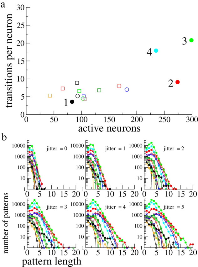
Data from all experimental datasets. a, A scatter plot showing the number of transitions per neuron versus the total number of active neurons. Each dataset is represented by a different symbol. The datasets given by the solid circles are those for which pairwise interactions are needed to reproduce the distributions of repeating patterns. They are also numbered 1–4 for ease of reference in the text. Note that the dataset from Figure 1 is given by the solid blue circle (dataset 4). b, The pattern distributions as in Figure 1b for all datasets and for different jitters. The symbols correspond to the datasets shown in a.

Pattern distributions

Patterns are defined as sequences of transitions from down to up states with a maximum duration of 50 frames (5 s) that occur at least twice (we do not quantify the number of repetitions of each pattern in this work beyond this criterion). For each dataset, we count all patterns of a given length, from 2 up to a length of 20. Length here refers to the number of neurons participating in the pattern, and not the number of down-to-up transitions, nor the number of repetitions of the pattern.

We use the template-matching algorithm described by Ikegaya et al. (2004). Briefly, given a reference cell c₁ and a reference transition time t₁, a vector (c₂, … , c_M, t₂, … , t_M) is constructed that contains all M − 1 transitions occurring within 50 frames (5 s) of the reference transition. Here, c_i is the index of the ith cell undergoing a transition (the same cell may undergo several transitions within the same 50 frame time window), and t_i is the time at which this transition occurs. The template (c₁, c₂, … , c_M, t₁, t₂, … , t_M) is then shifted to the next transition of the cell of reference. Any transitions that line up with the template now constitute a pattern. If j frames of jitter are allowed, then transitions that can be shifted by j or fewer frames to line up with the template constitute a pattern. Note that once jitter is allowed, the repeat of a pattern may include activations whose order is reversed. Thus, for example, with two frames of jitter the pattern (c₁, c₂, t, t + 1) would be considered a repeat of the pattern (c₁, c₂, t′, t′ − 1) (as would patterns with a transition of c₂ at times t − 3, t − 2, t − 1, and t). We now include a simple example to illustrate the process. Let us assume neuron c₁ = 2 undergoes a transition at time t₁ = 100. Then we look for all of the transitions occurring between times 100 and 150. These might be of cells c₂ = 1, c₃ = 20, and c₄ = 11 at times t₂ = 105, t₃ = 149, and t₄ = 149. Here, M = 4. These transitions now constitute our template. Let us now further assume that the subsequent transition of neuron c₁ = 2 occurs at t₁ = 200. The cells that undergo transitions between times 200 and 250 are c₂ = 1, c₃ = 20, and c₄ = 8. These transitions occur at times t₂ = 205, t₃ = 249, and t₄ = 249. We see that there is a three-neuron pattern (c₁, c₂, c₃) that has repeated with zero jitter (J = 0). The transition at time t₄ does not participate in the pattern, because in the template it is cell 11, whereas in the current 50 frame window it is cell 8.

Model

The model consists of N binary neurons, and the time evolution is discrete, with each time step representing Δt = 100 ms, and the total time is T. At any time step, each neuron may or may not undergo a transition to the up state. We consider four variants of the model: (1) independent Poisson neurons with a refractory period and stationary rates; (2) independent Poisson neurons with a refractory period and nonstationary rates; (3) stochastic binary neurons with a refractory period, stationary spontaneous rates, and probabilistic pairwise interactions; and (4) stochastic binary neurons with a refractory period, nonstationary spontaneous rates, and probabilistic pairwise interactions. Below, we describe each model in detail and explain how they can be fit to the experimental data.

(1) Stationary Poisson model

This model has the following parameters: (1) p̂_i ≡ the probability that neuron i will become active spontaneously; and (2) τ_r ≡ the effective refractory period, which is an integer greater than or equal to zero. These parameters can be estimated straightforwardly from the data. If the number of transitions of neuron i in the dataset is given by n_i, then the transition rate ν_i = n_i/T, where T is the total number of frames. The Poisson rate is given by p̂_i = ν_i/(1 − ν_iτ_r), where the refractory period τ_r is read off from the intertransition interval (ITI) distribution (see Fig. 1 and supplemental Figures S.7–S.20, available at www.jneurosci.org as supplemental material). Note that this model is guaranteed to reproduce mean transition rates. The ITI distribution of a Poisson neuron with a refractory period is just an exponential with an offset equal to the refractory period. Figure 1d (inset) shows that the ITI distribution averaged over all neurons in dataset 4 is not exponential, because it is not a straight line on a log-lin scale. This fact can be explained by noting that the ITI distribution summed over many Poisson neurons with different rates is a weighted sum of exponentials with different exponents (see an example in supplemental material, available at www.jneurosci.org).

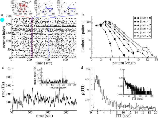
Figure 1.

Example of one experimental dataset. a, Raster plot in which each dot represents a transition from a down state to an up state in a cortical cell. Color-coded insets, Blowups of the raster plot in which repeated patterns are indicated. The six-cell pattern (in red) repeats after a few seconds, whereas the five-cell pattern (in blue) does so after several hundred seconds. b, The number of occurrences of repeating patterns as a function of pattern length. Shown are distributions for jitters of between 0 and 5 (see symbols in legend). c, The time-varying rate of transitions, calculated with a running average of 500 ms (5 bins). Inset, Mean transition rate for each neuron. d, The ITI distribution for all cells. An offset of ∼1 s (10 bins) is indicated by the dashed line. Inset, The same distribution on a log-lin scale.

(2) Nonstationary Poisson model

Same as 1 with the exception that the rates ν_i = ν_i (f) now depend on the frame f. This is done by calculating a 600 frame (1 min) sliding average, which assumes a very slow drift in the underlying rates.

(3) Stochastic model with interactions and stationary spontaneous rates

In this model, we still assume that the neurons can spontaneously undergo transitions. However, in addition we now allow for pairwise interactions between neurons. In particular, the model has the following parameters: (1) p̂_i ≡ the probability that neuron i will become active spontaneously at each time step; (2) τ_r ≡ the effective refractory period, which is an integer greater than or equal to zero; and (3) p_ij ≡ the excess probability that neuron i will become active at time step n + τ_d because of neuron j being active at time step n, where τ_d is the delay in the interaction and is an integer drawn randomly from 1 to w, where w is the maximum latency. The challenge in fitting this model to the data consists of estimating the interaction probabilities p_ijs and the maximum delay w.

Interaction probabilities p_ij.

Here we take a very simple approach. For each pair of neurons (i, j), we count the number of times in the dataset that a transition of neuron j coincides or is followed by a transition of neuron i within w frames. This yields an integer value for the number of coincident transitions C_ij. If neurons i and j were independent Poisson processes, then we could calculate the expected value of C_ij. If the number of transitions of neuron j is n_j, then the mean number of coincident transitions with neuron i is just n_jν_i where ν_i = n_i/T is the rate of neuron i. Counting coincidences with a time lag of 0 to w gives

If the C_ij from the data is significantly larger than μ_ij, then we assume there is an effective interaction between neurons i and j. Given that the datasets we work with contain relatively few transitions, we consider “significantly larger” to mean greater than one SD from the mean. We thus take

where |x|₊ = x if x > 0 and is zero otherwise, and β = 1. Here we take the variance in the number of coincident transitions C_ij to be σ_ij² = μ_ij. This is a good approximation when the mean ITI of the neurons is much greater than the refractory period. This formula means that the probability of neuron j causing a transition in neuron i is just the fraction of excess coincident transitions in the data compared with the mean plus one SD of independent Poisson neurons. Equation 2 can then be thought of as an ansatz that is applied to the data, allowing us to extract the p_ijs directly. Finally, we note that if C_ij ≤ 2, then p_ij is set to zero. Examples of the distribution of C_ijs in datasets 1–4 as well as a graphical interpretation of Equation 2 can be found in section 2 of the supplemental material (available at www.jneurosci.org).

Maximum delay w.

To apply Equations 1 and 2, we must furthermore choose a value for w. A value of w = 5 was chosen by inspecting changes in the ITI distribution within patterns for different values of the jitter. The most pronounced changes occurred in approximately the first five frames, indicating that sequences of activations with latencies greater than this were most likely attributable to chance. Note that several datasets exhibited too few patterns to accurately measure this effect. In principle, the parameters β and w could be allowed to vary, potentially resulting in better fits, although this has not been systematically explored. The fits we present here have, in fact, not been systematically optimized as a function of this or any other parameter.

Once the p_ijs have been estimated in this way, the spontaneous rates p̂_i are calculated to ensure that the mean rate for each neuron in the simulation matches the rate of the corresponding neuron in the dataset. This is done in the following way. For a neuron i in the model, the probability of undergoing a transition can be approximated by

where the first term is the probability of spontaneous activation, and the second term is the probability that a presynaptic neuron j causes a transition, summed over all neurons j. Equation 3 is a good approximation when the rates ν_i and transition probabilities are small. The rate of neuron i, ν_i, is just p̂_i divided by a factor, >1, which takes into account the refractory period

Finally, we now rewrite Equation 4 for p̂_i, which yields

In the model, we assume that the “postsynaptic” neuron undergoes a transition τ_d frames after the “presynaptic” neuron, where τ_d is uniformly distributed between 1 and w. A simpler choice would be to render the model Markovian, i.e., τ_d = 1 always. However, such a model fails to produce pattern statistics consistent with those found in experiments. Indeed, the latency between subsequent transitions within a pattern most often is >1, indicating that, if neuronal interactions are present, their effect is felt over several hundred milliseconds. Because we assume in Equation 2 that interactions occur within a window w, the weakest assumption we can make concerning the delay is that it is uniformly distributed within that window. This choice furthermore results in a cross-correlogram of the simulated transitions with a width that agrees qualitatively with that of the experimental data (for an example, see supplemental Figure S.6, available at www.jneurosci.org as supplemental material). We also conducted simulations with a probability distribution for the delay that decays in time, leading to results qualitatively similar to the case with a uniform distribution. This suggests that the crucial property of the delay in the interactions is the time scale (hundreds of milliseconds) and not the precise form. See supplemental material (available at www.jneurosci.org) for details of these simulations. Note also that although we consider coincident transitions in calculating the p_ijs, we do not allow τ_d to be zero in the simulations for simplicity.

(4) Stochastic model with interactions and nonstationary spontaneous rates

Same as 3 with the exception that the rates now depend on the frame f. Now we have

and again σ_ij² = μ_ij. The spontaneous rates are given by

where p_ij is given by Equation 2.

Goodness of fit

We test the similarity between the pattern distributions and those obtained from simulations of the model. To do so, we first fit the model as described in the preceding section. We then perform n simulations of the model, thereby generating n simulated datasets. We count the number of patterns for each of these n simulated datasets. We then calculate the measure

where e_i(J) is the number of patterns of length i in the experimental dataset for a jitter J. Similarly, s_i^μ(J) is the number of patterns of length i in the μth simulated dataset for a jitter of J, whereas σ_i(J) is the SD of this value over all n simulations. Here, n = 100.

Because the number of realizations of the simulated data are finite, for long enough pattern lengths the number of patterns determined numerically will be identically equal to zero. In light of this, to allow for arbitrary pattern length in calculating d, we must estimate the variance σ_i²(J) when s_i^μ(J) = 0 for all μ. We do this by assuming an exponential dependence in the mean number of patterns as a function of pattern length, which is approximately consistent with the experimental and simulated data. Thus, we take E(s_i) = E(s_i−1)²/E(s_i−2), and the variance is then taken to be σ_i²(J) = E[s_i(J)](1 − E[s_i(J)]/n), which assumes a binomial distribution, i.e., a fixed probability E[s_i(J)]/n of finding a pattern on each realization. Once we have extrapolated σ_i²(J) in this way to all is, we can calculate d(J) for any value of N. However, we note that if for a given i both e_i and s_i^μ(J) (for all μ) are identically equal to zero, then the corresponding contribution to the sum will be zero. The value of d will thereby decrease because of the normalizing factor N, i.e., one can obtain arbitrarily low d by taking N large enough. Thus, to avoid spuriously low values of d, rather than choosing an arbitrary N to calculate d(J), we take the value of N for which e_N+1 first reaches zero.

If the underlying stochastic process for the experimental and simulated data were the same, then for a sufficiently large number of realizations of both we would have d(J) ∼ 1, because e_i(J) = μ(J) + σ_i(J)ξ_e and s_i(J) = μ(J) + σ_i(J)ξ_s, where ξ_e and ξ_s are uncorrelated random variables with unit variance. That is, the mean and variance of both processes are the same. Plugging these formulas into Equation 8, we find lim d(J) → 1 as the number of realizations grows. Because we only have one “realization” of the experimental data, we should expect that d(J) differ from 1 even given identical stochastic processes. As an example, if the number of patterns found in the data were exactly equal to the mean of the stochastic process described by the simulations, i.e., e_i = E(s_i), for all pattern lengths i, then d(J) = 0.5 exactly. On the other hand, an outlier value of e_i for just one i can lead to a large value of d(J). We must therefore assume that the numbers of patterns found in the data are actually representative of the underlying random process; i.e., we assume that large values of d(J) indicate distinct processes. Conservatively, then, we can say that if d(J) is of order 1, then the pattern distributions are approximately consistent with those generated by the model. Although d(J) provides a means of quantifying the goodness of fit for analysis, we also include the fits of all four models to all datasets for all patterns lengths i and all jitters J (see supplemental Figures S.21–S.32, available at www.jneurosci.org as supplemental material).

Drawing randomized matrices

We test three types of randomized surrogate matrices: (1) randomized connections within the full matrix, (2) randomized connections within the connected subgraph, and (3) randomized connections keeping the degree distribution intact. In each case, we assume that there are N neurons and k nonzero connections between neurons, where k ≤ N (N − 1) (self-connections are not allowed). For datasets 1–4, in fact, k ≪ N(N − 1), i.e., the connectivity is sparse.

(1) We designate each connection in the original matrix by the pair Π_l = (i, j), l ∈ {1, … , k}, where i and j are the postsynaptic and presynaptic neurons, respectively. For each connection, we then generate two random integers, a and b, uniformly distributed between 1 and N, but excluding self-connections and multiple connections, i.e., a ∈ {1, … , N}, b ∈ {1, … , N}, b ≠ a. We then rewire this connection such that Π_l = (a, b). We repeat this procedure for all k connections.

(2) We first identify the neurons that neither receive nor send out any connections; i.e., they are unconnected. Mathematically, a neuron u is unconnected if Σ_j=1^N(p_uj + p_ju) = 0; i.e., there are no incoming nor outgoing connections. If there are N − N′ unconnected neurons, then we can define a subgraph of the original matrix, which consists of only N′ ≤ N neurons, all of which are connected. The subgraph contains all of the connections present in the original matrix. We now work with the connected subgraph of N′ neurons and k connections and conduct the random rewiring as in 1 above.

(3) The degree distribution of a graph is the distribution of links at each node. In a directed graph such as the ones we consider, one can define an in-degree and an out-degree distribution, which refer to incoming and outgoing connections, respectively. For datasets 2–4, we have numerically calculated the in-degree and out-degree distributions (see Fig. 10). To these, we have fit analytical expressions ρ_in(k) and ρ_out(k). These expressions can be interpreted as the probability of choosing a neuron at random and finding that it has k incoming and outgoing connections, respectively. We can make use of ρ_in and ρ_out to generate randomized matrices from datasets 2–4 while keeping the degree distribution intact. We first define two vectors of length N, x and y, where the elements of the vectors are random numbers drawn from ρ_in and ρ_out, respectively, i.e., x is distributed according to ρ_in and x_i is an integer that is a particular sample from ρ_in and represents the number of incoming connections to neuron i. Analogously, y is distributed according to ρ_out, and y_i represents the number of outgoing connections from the same neuron i. We now have two copies of each neuron, one with incoming connections and one with outgoing connections. The total number of incoming and outgoing connections is I = Σ_i=1^Nx_i and O = Σ_i=1^Ny_i, respectively. Generically, we will find that I ≠ O. To enforce the self-consistent condition I = O, we selectively prune away and add on connections. If I > O, then we choose a neuron i at random, and with a probability 0.5, we eliminate one incoming connection with a probability p = x_i/I, i.e., x_i → x_i − 1. Otherwise we add one outgoing connection with a probability p = y_i/O, i.e., y_i → y_i + 1. We continue this procedure until I = O. If O > I, we prune away outgoing connections and add on incoming connections in an analogous way. We have checked numerically that the pruned and augmented x and y continue to be distributed according to ρ_in and ρ_out, respectively. Once I = O, we choose an incoming connection and an outgoing connection at random, excluding self-connections and multiple connections. If they are from neurons i and j, then this represents a pair Π_l = (i, j), where l ∈ {1, … , I}. We repeat this procedure for all I connections. This results in a matrix in which the connections have been randomized, but the in-degree and out-degree distributions have not changed.

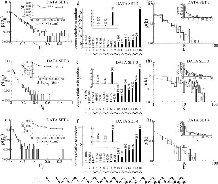
Figure 10.

Properties of the graphs of interactions. a, The distribution of p_ijs for dataset 2. Note the log-lin scale. Inset, The probability of connection as a function of distance averaged over all pairs of neurons. The probability of connections decreases only weakly with distance. b, As in a for dataset 3. c, As in a for dataset 4. d, Network motifs for dataset 2. Shown is the ratio of the number of motifs compared with that found in a random network. As in the study by Song et al. (2005), the null hypothesis is generated by assuming independent connection probabilities. Inset, Doublets. Main panel, Triplets. A blowup of the triplet motifs is shown at the bottom of the figure. e, As in d for dataset 3. f, As in d for dataset 4. g, The degree distributions (solid line, in distribution; dotted line, out distribution) ρ(k) for dataset 2. Note the log-log scale, and see inset for a linear scale. A suggestive fit to a truncated power law distribution is indicated by the dashed line. See Results. h, As in g for dataset 3. i, As in g for dataset 4.

So far, we have only discussed the presence or absence of a nonzero p_ij and not the actual value itself. In all cases 1–3, nonzero weights p_ij are set to be a randomly reshuffled version of the original weight matrix.

Results

We first discuss the experimental data, then the fit of the model to the data, and finally the properties of the resulting matrices of interactions p_ij.

Experimental data

We study 15 datasets of varying numbers of neurons and varying durations. An example of a dataset is shown in Figure 1. Figure 1a shows the “raster” plot of transitions from a dataset 4 with 243 neurons (Fig. 2a, solid cyan circle). From the naked eye, it seems that some neurons undergo more transitions than others, i.e., rates vary across neurons, and that for some neurons the rate of transitions changes in time. This is typically seen in most datasets. Our focus here, however, will be on the statistics of repeating patterns of activity, two examples of which are shown in Figure 1a. Length-6 (i.e., the pattern is made up of six transitions) and length-5 patterns are shown in red and blue, respectively, in the insets. Whereas the red pattern repeats after several seconds, the blue pattern does so after several hundred seconds. We counted all patterns ranging from length 2 to length 20 that occurred at least twice in this dataset. The resulting distribution is shown in Figure 1b for five values of the jitter in the replay or repetition of the pattern. We have included the total transition rate as a “length-1” pattern to constrain the models to reproduce the total number of transitions; i.e., the model should reproduce, on average, both the distribution of patterns and the total number of transitions. The trend is clearly for larger numbers of patterns with increasing jitter. Figure 1c shows the transition rate of the dataset, averaged over all neurons, as well as the mean transition rate of each neuron (inset), whereas Figure 1d shows the ITI distribution. The ITI distribution is set off from zero as indicated by the vertical dashed line. This offset is taken as the effective refractory period in the model for the neurons in this dataset. The sharp decrease in the ITI distribution for short ITIs (see inset) is consistent with independent Poisson processes with heterogeneous underlying rates [see Materials and Methods and supplemental material (available at www.jneurosci.org)]. See supplemental material (available at www.jneurosci.org) for the equivalent of Figure 1 for the remaining 14 datasets.

There are significant variations in rates and pattern statistics in the experimental data as indicated by Figure 2. Figure 2a is a scatter plot in which each symbol indicates the number of active neurons and mean number of transitions per neuron in one of the 15 corresponding datasets. The number of active neurons, defined as neurons exhibiting at least one transition, ranges from 43 to 299, whereas the number of transitions per neuron ranges from slightly less than 3 to more than 20. Note that the dataset featured in Figure 3 of Ikegaya et al. (2004) is given here by dataset 1. Pattern distributions for values of the jitter between 0 and 5 are shown in Figure 2b. The symbols correspond to the datasets shown in Figure 2a; this convention will be used in the figures that follow. The four datasets for which we find a significant effective interaction between neurons are denoted by the solid circles and are additionally labeled 1–4 for ease of reference in later sections.

Figure 3.

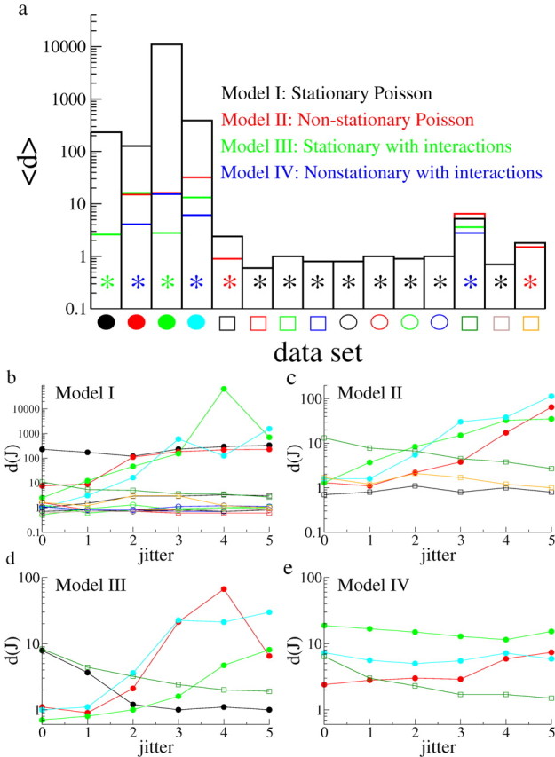
Goodness of fits of the models to the data. a, The average value of the goodness of fit d over all jitters for each dataset. Values of d of order 1 indicate a good fit. Black bars, Values obtained from a fit of the stationary Poisson model with refractory period. Red bars, Nonstationary Poisson model with refractory period. Green bars, Stochastic model with interactions and stationary spontaneous rates. Blue bars, Stochastic model with interactions and nonstationary spontaneous rates. The model providing the best fit is indicated for each dataset by an asterisk of the corresponding color. Datasets are represented by the same symbols as in Figure 2. Eight of the 15 datasets are best described by a Poisson model with stationary rates and a refractory period, whereas two are best described by a nonstationary Poisson model. Of the remaining five, two are best described by the stochastic model with interactions and stationary rates, whereas three are better described by the stochastic model with interactions and nonstationary spontaneous rates; however, for one dataset (open yellow square), the improvement in the goodness of fit from the model with interactions is marginal compared with the Poisson model. b, The goodness of fit d(J) as a function of jitter for the stationary Poisson model. Each curve is a dataset, given by the corresponding symbol. c, Same as b but for the nonstationary Poisson model. Only datasets not well fit by the stationary Poisson model are shown. d, Same as b for the stochastic model with stationary spontaneous rates. Only datasets not well fit by a Poisson model are shown. e, Same as d but with nonstationary spontaneous rates. Only datasets not well fit by a Poisson model are shown.

Fits of the model

We seek the simplest possible model that can successfully reproduce data such as those shown in Figures 1 and 2. Given the irregularity of the activity seen in all datasets, it seems reasonable to choose a stochastic model in which transitions occur probabilistically. This is furthermore consistent with the notion of patterns that may repeat imperfectly because of jitter in the transition times. We will consider four variants of a stochastic model: (1) a stationary Poisson model, (2) a nonstationary Poisson model, (3) a model with pairwise interactions and stationary spontaneous rates, and (4) a stochastic model with pairwise interactions and nonstationary spontaneous rates. See Materials and Methods for details of each model. In all models, there is an effective refractory period, estimated from the offset in the ITI distribution as shown in Figure 1d. This reflects, to some extent, the fact that once a cell has undergone a transition to an up state, it will reside there for some time before dropping back to the down state.

All four of the models listed above can be fit to each dataset straightforwardly (see Materials and Methods). Once a fit has been made, simulated datasets can be generated and the pattern distributions determined. These distributions are then compared with the experimental ones, and a goodness of fit for each value of the jitter d(J) is estimated (see Materials and Methods). For this particular measure, d(J) of order 1 indicates a good fit. Figure 3a shows the goodness of fit 〈d〉, where the brackets indicate an average over jitter.

The first striking feature of this graph is that the datasets can be sharply divided in two categories: for the four datasets shown on the left, the stationary Poisson model provides a very bad fit of the data, with 〈d〉 > 100. For the remaining 11 datasets, the stationary Poisson model provides a much better fit, with 〈d〉 < 10. We first examine the datasets that are best fit by the Poisson model. In fact, the value of 〈d〉 for the stationary Poisson model (black) is in the range [0.6–1.0] for 8 of these 11 datasets, as indicated by the black asterisk. The three remaining datasets have 〈d〉s in the range [1.8–5.2]. The nonstationary Poisson (red) model improves the quality of fit for two of these datasets, providing 〈d〉s of 0.9 and 1.5, respectively (datasets indicated by red asterisk). For the last of these datasets (open dark-green square), the nonstationary model with interactions provides the best fit to the data, but there is only a minor improvement in the goodness-of-fit measure between this model and the Poisson model. We therefore do not consider this dataset further.

We now turn to the four datasets that are very poorly fit by the stationary Poisson model (solid circles). In all these datasets, adding interactions very strongly improves the quality of the fit, with resulting 〈d〉s in the range [2.6–6.1]. Two are best fit by a model with stationary spontaneous rates (datasets 1 and 3) and two by a model with nonstationary spontaneous rates (datasets 2 and 4). Note that dataset 1 is too short in duration to allow for any nonstationarities (T = 60 s). The poorer fit of the nonstationary model to dataset 3 compared with the stationary model is likely a result of overfitting. Specifically, the nonstationary model fits a deterministic change in rates to what are most likely stochastic fluctuations.

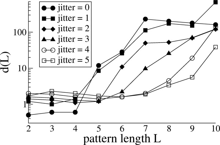
Figure 3b–e shows the goodness of fit d(J) as a function of jitter for the four models (1–4, respectively). Note that with the exception of the dataset 1, all datasets are consistent with a Poisson process (Fig. 3a,b) for low values of jitter. Indeed, d(J) is of order 1 for J = 0, 1 in this case. This suggests that the occurrence of precisely repeating patterns is entirely explained by independent Poisson processes. This is not the case if we consider greater degrees of jitter, where pairwise interactions between neurons are needed to account for pattern statistics (Fig. 3c,d). In addition, if we look at the goodness of fit as a function of pattern length, we find that short patterns can be explained by independent Poisson processes. Figure 4 shows the goodness of fit of the stationary Poisson model to dataset 1 as a function of the pattern length L. Only patterns involving five or more neurons cannot be captured by this model. This suggests that activity resulting from recurrent connections between neurons tends to generate noisy patterns that both are long and typically do not repeat exactly.

Figure 4.

Goodness of Poisson fit as a function of pattern length. The goodness of fit as a function of pattern length d(L) of the stationary Poisson model is shown as a function of the pattern length for dataset 1. We chose this dataset as exemplary because it is the only one for which low-jitter patterns are not captured by a Poisson model and therefore provides the strongest test of the Poisson hypothesis. Note that d(L) is of order 1 for short patterns (L < 5).

The datasets for which interactions are estimated to be present (except for dataset 1) all contain considerably more data than the other datasets. It may be that pattern statistics that deviate from those generated by a Poisson process with refractory period are only detectable given a sufficiently large dataset. To investigate this, we broke sets 2–4 into smaller subsets of data: two subsets for dataset 2 and four subsets for each of the datasets 3 and 4. This yielded a total of 10 datasets from the original three, which we then fit with the stationary and nonstationary Poisson models. In 7 of the 10 cases, the nonstationary Poisson model provided a much better fit than the original datasets 〈d〉 < 10), whereas for 3 subsets, neither Poisson model increased significantly the quality of fit (see section 2 and supplemental Figs. S.2–S.5, available at www.jneurosci.org as supplemental material). This suggests that the good fit of a Poisson model to the 11 original datasets may be, in part, explained by a lack of data. Thus it may be that had more data been available, the distributions of repeating patterns would only have been reproduced by a model with interactions.

Properties of the interaction matrices

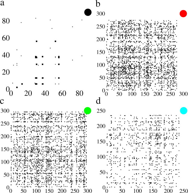
Here we study the properties of the matrices p_ij estimated for datasets 1–4, which are reasonably well fit by a stochastic model with pairwise interactions. Figure 5 shows the connectivity matrix for each of the four datasets in which a filled entry indicates a nonzero p_ij for that pair, j on the x-axis and i on the y-axis. The identity of the dataset is indicated by the corresponding symbol. Figure 5a shows the connectivity of dataset 1. Of a total of 83 active neurons, 19 form a connected subgraph of 46 links. The degree of connectedness (the number of connections divided by the total number of possible connections) within this subgraph is therefore 13%. In addition, we have highlighted those connections for which p_ij > 0.5 by enlarging the corresponding square. This reveals a strongly interconnected subnetwork of neurons (neurons 6, 13, 29, 30, 37, 38, and 56). The matrices in Figure 5b–d are all qualitatively similar to one another. The connectivity is relatively diffuse with no obvious structure. However, all three matrices exhibit vertical and horizontal “stripes,” which indicate that some neurons receive a large number of outgoing and incoming connections; i.e., they connect broadly across the network. The degree of connectedness within the connected subgraph is 3.1, 5.5, and 4.5% for datasets 2, 3, and 4, respectively.

Figure 5.

Network topology extracted from the analysis. The matrix topology of the four datasets for which a nonzero connectivity was estimated is shown. The matrix entry is filled in by a black square wherever p_ij is nonzero. This therefore shows the presence of a connection but not its strength. In each case, the dataset is indicated by the corresponding symbol. a (solid black circle), A very sparse matrix (0.7% connection probability). However, only 19 neurons actually form a connected subgraph, yielding a connection probability of 13%. The strongest connections p_ij > 0.5 form a strongly interconnected subgraph of their own, here shown by slightly enlarged squares. See Results. b (solid red circle), The sparseness within the connected subgraph is 3.1%. Visible are horizontal and vertical striations indicating neurons with a high degree of incoming and outgoing connections, respectively. c (solid green circle), The sparseness within the connected subgraph is 5.5%. Visible are horizontal and vertical striations indicating neurons with a high degree of incoming and outgoing connections, respectively. d (solid cyan circle), The sparseness within the connected subgraph is 4.5%. Visible are horizontal and vertical striations indicating neurons with a high degree of incoming and outgoing connections, respectively.

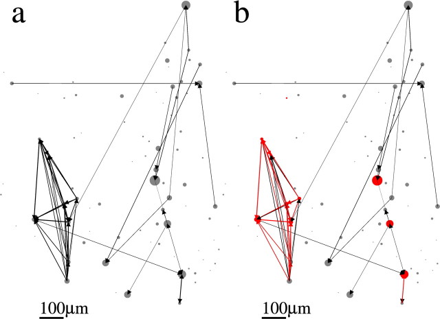
Figures 6–9 show the spatial topology of the estimated connectivities for datasets 1–4. Circles indicate the actual spatial location of each neuron in the slice, where the diameter of the circle is proportional to the transition rate of each neuron. Arrows indicate the presence of a nonzero p_ij, and the width of the arrow is proportional to the value of p_ij. Figure 6a shows that connections span the entire network, although a highly spatially structured subnetwork of neurons is apparent in the bottom left part of the slice. This spatially localized subnetwork is, in fact, made up of the most strongly connected neurons. This is illustrated in Figure 6b, in which all of the connections for which p_ij > 0.5 are colored in red. We also colored those neurons in red that make up the long length-10 pattern observed and shown in Figure 3A of Ikegaya et al. (2004). It is clear that the neurons with p_ij > 0.5 are those that are primarily responsible for the generation of this pattern. The spatial topology of the remaining three datasets appears qualitatively similar (for datasets 2–4, see Figs. 7–9, respectively). The networks are broadly connected, and no obvious spatial structure is present (Figs. 7a, 8a, 9a). We also show the topology of the strongest connections p_ij > 0.2 in Figures 7b, 8b, and 9b. Note that in contrast to Figure 6b, in which the strongest connections formed a spatially localized subnetwork, here they are spatially unstructured, as in Figure 7b, or strong connections are nearly absent, as in Figures 8b and 9b. In fact, the network topology for datasets 2–4 always appears spatially unstructured to the eye for any threshold value of p_ij.

Figure 6.

Spatial organization of networks of dataset 1. The spatial position of each neuron in the slice is represented by a circle. The diameter of the circle is proportional to the rate of transitions from the down to the up state in the corresponding neuron. Arrows indicate a nonzero p_ij as estimated from the model. The thickness of the arrow is proportional to the value of p_ij. Scale bar, 100 μm. a, Full topology. b, Connections for which p_ij > 0.5 are colored in red. These strong connections clearly form a spatially localized subnetwork of neurons. Those neurons participating in the length-10 pattern are shown in red and correlate strongly with the spatially localized subnetwork.

Figure 7.

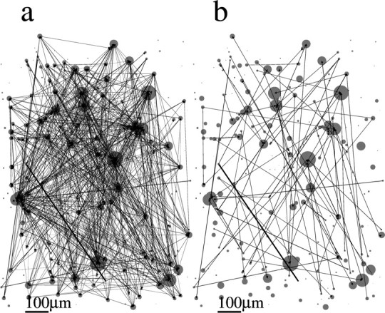
Spatial organization of networks of dataset 2. The spatial position of each neuron in the slice is represented by a circle. The diameter of the circle is proportional to the rate of transitions from the down to the up state in the corresponding neuron. Arrows indicate a nonzero p_ij as estimated from the model. The thickness of the arrow is proportional to the value of p_ij. Scale bar, 100 μm. a, Full topology. b, Only connections with p_ij > 0.2.

Figure 8.

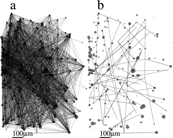
Spatial organization of networks of dataset 3. The spatial position of each neuron in the slice is represented by a circle. The diameter of the circle is proportional to the rate of transitions from the down to the up state in the corresponding neuron. Arrows indicate a nonzero p_ij as estimated from the model. The thickness of the arrow is proportional to the value of p_ij. Scale bar, 100 μm. a, Full topology. b, Only connections with p_ij > 0.2.

Figure 9.

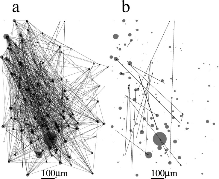
Spatial organization of networks of dataset 4. The spatial position of each neuron in the slice is represented by a circle. The diameter of the circle is proportional to the rate of transitions from the down to the up state in the corresponding neuron. Arrows indicate a nonzero p_ij as estimated from the model. The thickness of the arrow is proportional to the value of p_ij. Scale bar, 100 μm. a, Full topology. b, Only connections with p_ij > 0.2.

Further characterization of the interaction matrices for datasets 2–4 is shown in Figure 10. Figure 10a–c shows the distribution of p_ijs, which is approximately exponential in all three cases. The probability of connection as a function of distance is shown in the inset. Error bars are SEs. Figure 10, d and f, shows the ratio of the number of various types of doublet (inset) and triplet connection motifs to the number of motifs in a network in which connection probabilities are independent, as in Song et al. (2005). Here, only the topology of the network is considered, i.e., the presence or absence of a nonzero p_ij and not the value of p_ij itself. Each type of motif is indicated by a corresponding diagram. A blowup of the different triplet motifs is shown at the bottom of Figure 10. The actual number of motifs found in each case is given above each bar. In all three cases, we find an overrepresentation of both bidirectional connections as well as the more highly connected triplet motifs. These findings are approximately consistent with results from simultaneous, multiple intracellular recordings in cortical slices (Song et al., 2005).

The degree distribution ρ(k) gives the probability of choosing a neuron in a network at random and finding k links (Albert and Barabási, 2002). Figure 10g–i shows the degree distributions for both incoming (solid lines) and outgoing (dotted lines) connections. The insets show the histograms on a linear scale. The distributions are approximately consistent with a truncated power law given by ρ(k) ∼ 1/k, for Figure 10, g and i, and ρ(k) ∼ 1/k^1/2 for Figure 10h (see dashed lines).

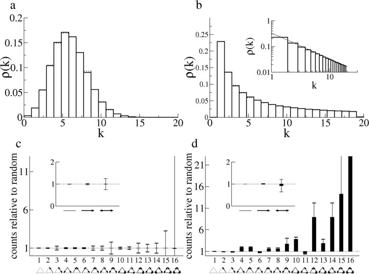
The degree distribution and distributions of doublet and triplet motifs are not independent. Indeed, the null hypothesis used to calculate the number of motifs relative to random in Figure 10d–f is that connections are made randomly with a fixed probability. This prescription for making connections would result in a binomial degree distribution, which is clearly inconsistent with the monotonically decreasing distributions seen in Figure 10g–i. We explore to what extent the deviation of the distribution of doublet and triplet motifs is attributable to the form of the degree distribution. To do so, we generate 100,000 networks by laying down connections randomly with a probability of 0.035 and 100,000 networks with a truncated power-law degree distribution given by ρ(k) ∼ 1/k. These values result in a similar mean degree for both networks 〈k〉 ∼ 6. In both cases, we take a system size equivalent to the connected subgraph of dataset 2 (161 neurons). Histograms of the degree of incoming (solid lines) and outgoing (dotted lines) connections for the random and power-law networks over all 100,000 realizations can be seen in Figure 11, a and b, respectively. The inset in Figure 11b shows the agreement of the theoretical degree distribution ρ(k) used to generate the networks to the histogram. Figure 11, c and d, shows the number of doublet and triplet motifs for the purely random and power-law networks averaged over 100,000 realizations. Error bars indicate the SD of fluctuations in the numbers of motifs across realizations resulting from the finite size of the networks. We have checked that after 100,000 realizations any error in the measurement of the mean or SD is negligible. It can be seen from Figure 11c that the network motifs are consistent with a random graph, as should be the case. Figure 11d indicates that not all of the features of the overrepresentation of doublet and triplet motifs in Figure 10e–g can be explained by the presence of a power-law degree distribution. In particular, there is no overrepresentation of doublet motifs. Furthermore, the overrepresentation of triplet motifs seems to directly reflect the increased amount of convergence and divergence related to nodes with large degree, or “hubs.” Note, in particular, that triplet motifs 6 and 11, which involve clockwise or counterclockwise chains of connections, are not overrepresented. This can be contrasted with patterns 4, 5, 7–10, and 12–16, all of which involve patterns of convergent or divergent connections. The overrepresentation of bidirectional doublets and certain triplet motifs in the three datasets we are considering therefore reflects additional structure in the network topology beyond the degree distribution alone.

Figure 11.

Doublet and triplet motifs for random networks with binomial or power-law degree distributions. a, Histogram of the degree of incoming (solid lines) and outgoing (dotted lines) connections in 100,000 networks of 161 neurons in which connections are made with a fixed probability of p = 0.035. b, Histogram of the degree of incoming (solid lines) and outgoing (dotted lines) connections in 100,000 networks of 161 neurons generated from a truncated power-law degree distribution. Inset, Log-log plot of the same histogram and the function used to randomly generate the degree of connections (dashed line), ρ(k) ∼ 1/k. c, The number of doublet and triplet motifs in the random network compared with that predicted from a random network. Values are averaged over 100,000 realizations, and error bars show one SD (see Results). d, The number of doublet and triplet motifs in the network with power-law degree distribution compared with that predicted from a random network. Values are averaged over 100,000 realizations, and error bars show one SD (see Results).

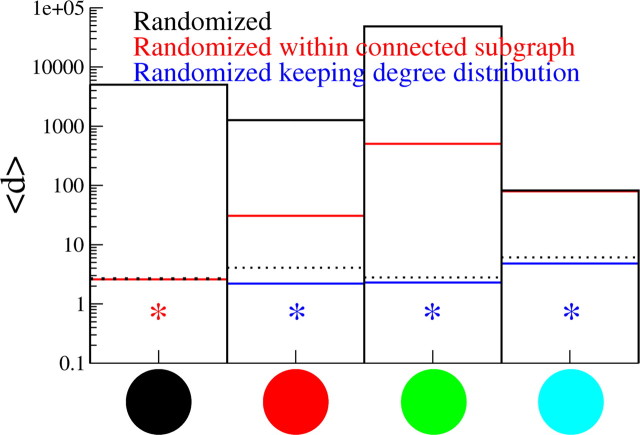
We may ask what properties of the interaction matrices lead to the distributions for the repeating patterns of activity that agree with the experimental data. In particular, if we can generate randomized surrogate matrices in which this property is preserved, we should also preserve the resulting pattern distributions. We test three different surrogate matrices. It may be that the distribution of weights p_ij alone (Fig 10a–c) is sufficient to generate the pattern distributions without any additional network structure. We test this hypothesis by rewiring each connection by choosing two neurons at random, one presynaptic and one postsynaptic, with equal probability from the total number of active neurons in the dataset. Among other effects, this will result in the elimination of any overrepresentation of motifs present. Figure 12 shows the goodness of fit averaged over jitters 〈d〉 for this particular surrogate, given by the black bar. The pattern distributions for this case are clearly altered.

Figure 12.

Goodness of fit of models with randomized connectivity. Goodness of fit d of models with randomized connectivity. Three randomization paradigms were tested for the connections p_ij: (1) within full graph, (2) only within the connected subgraph, and (3) within the connected subgraph while keeping the degree distribution intact. The pattern distributions were unchanged in dataset 1. Dotted lines show the goodness of fit for the original, best-fit model. See Materials and Methods for a description of how the randomized connectivities were generated. The model providing the best fit is indicated for each dataset by an asterisk of the corresponding color.

Second, we have noted earlier that not all active neurons are connected via incoming or outgoing connections to other neurons. It may be that the particular structure of the connected subgraph is of importance. To test this, we randomize connections by choosing two neurons at random from within the connected subgraph. The corresponding goodness of fit (red) shown in Figure 12 is close to 1 for dataset 1. Indeed, we saw previously that this dataset exhibits a small, highly interconnected subnetwork. This hypothesis is, however, insufficient to generate the pattern distributions for the remaining three datasets.

Finally, we consider the role of the degree distribution. As we have seen, in a standard Erdös-Renyi graph in which connections are laid down independently and with equal probability, the degree distribution is binomial and thus nonmonotonic; i.e., there is a “preferred” value k = pN, where p is the probability of connection and N is the size of the network (Albert and Barabási, 2002). The degree distributions in Figure 10g–i are clearly monotonically decreasing and exhibit long tails, indicating that the topologies of the interaction matrices do not form standard random graphs. To explore the role of the degree distribution in generating the statistics of repeating patterns, we randomize the connections by drawing random numbers from the power-law fit of the degree distributions shown by the dotted lines in Figure 10g–i. These random numbers are used to assign incoming and outgoing connections to neurons chosen at random from within the connected subgraph. The “ends” of the incoming and outgoing connections must then be “tied” together self-consistently (see Materials and Methods). Simulated pattern distributions using such interaction matrices agree well with the experimental data (Fig. 12, blue). We also constructed randomized matrices for which only the in- or the out-degree distribution is kept, whereas the other is seeded randomly and is thus binomial (data not shown). Neither of these hybrid topologies succeeds in generating the pattern statistics as well as the original matrix. Nonetheless, maintaining a power-law degree distribution of the outgoing connections does significantly better than the alternative scenario. This suggests that single neurons with a large number of outgoing connections significantly contribute to the generation of long, noisy patterns.

Discussion

The main goal of our study was to find a simple model capable of reproducing the statistics of the repeating patterns seen in calcium-imaging work in slice (Ikegaya et al., 2004). In 11 of the 15 datasets we analyze, a Poisson model with refractory period provides a good fit, whereas for the remaining four, the presence of pairwise interactions greatly improves the fit over a simple Poisson model. We have asked the question, what is it about the structure in the pairwise interactions that generates the repeating patterns in these four datasets? We have looked at several possibilities: the distribution of interaction strengths alone, the structure of the connected subgraph, and the degree distribution. For dataset 1, the structure of the connected subgraph appears crucial. For datasets 2–4, one can rewire connections randomly, as long as the in-degree and out-degree distributions are held intact, and obtain numbers of repeating patterns similar to those seen in the data. This means that there is a statistical ensemble of random networks that produce repeating patterns similar to those seen in experiments. This, in turn, suggests that one should be cautious in interpreting the functional usefulness of such repeating patterns.

Do repeating patterns of transitions between down states and up states occur above chance in the data we have studied? If we define chance as meaning “consistent with independent Poisson neurons with a refractory period” (our models 1 and 2), then in 11 of the 15 datasets repeating patterns do not occur above chance. In three of the remaining four datasets (datasets 2–4), short patterns and exactly repeating patterns (low jitter) do not occur above chance. In these datasets, long patterns with some jitter do occur above chance. Finally, in dataset 1, sufficiently long patterns occur above chance for any jitter. However, datasets 2–4 have both larger numbers of neurons and more transitions per neurons than the others. The fact that 11 of the remaining 12 datasets can be well fit by independent Poisson processes might therefore be attributable to the fact that there are simply not enough spikes to detect connectivity in those datasets. We have broken datasets 2–4 down into 10 smaller subsets and found that seven of them can be well fit by a Poisson model (see supplemental material, available at www.jneurosci.org). This suggests that the 11 experimental datasets whose distribution of repeating patterns can be explained by a Poisson model alone may have yielded nonzero interaction matrices had they been longer.

Having summarized our main findings, we would like to review the pedigree of the data we have analyzed to place our work in its proper context. The data were originally presented in a study in which repeating patterns of neuronal activity were found to occur on two distinct time scales (Ikegaya et al., 2004), as follows.

A time scale of milliseconds

In vitro recordings from mouse primary visual cortex and in vivo recordings from cat primary visual cortex revealed patterns of subthreshold voltage fluctuations that repeated with millisecond precision. The number of repeats was compared with the number of repeats in time-shuffled surrogate data series and found to be significantly larger. The surrogate time series was generated by thresholding the voltage traces, thereby keeping track of the largest postsynaptic potentials (PSPs), and then shuffling the intervals between PSPs. A more recent study looked at repeating patterns in subthreshold activity in in vivo recordings in rat barrel cortex and cat striate cortex (Mokeichev et al., 2007). The authors compared the number of repeats to repeats found in three types of surrogate data series: time-shuffled traces without thresholding, phase-randomized traces, and traces generated from a simple neuron model with Poisson inputs. In all three cases, they found that the surrogate data produced comparable numbers of repeats to the original data.

A time scale of hundreds of milliseconds to seconds

Calcium imaging recordings from primary visual and medial prefrontal cortex in mice showed repeating patterns of transitions from down to up states in cortical cells, which occurred on the time scale of hundreds of milliseconds to seconds. The number of repeating patterns found was compared with that found in three different types of surrogate datasets: (1) shuffling of ITIs within neurons, (2) shuffling of spikes across neurons, and (3) exchange of spikes across neurons. In all three cases, the authors found a significantly lower number of repeating patterns in the surrogate data.

Our work has revisited the calcium imaging data and shown that a simple stochastic model incorporating spontaneous activity, pairwise interactions, and a refractory period is sufficient to reproduce the distributions of repeating patterns. It is instructive to ask what the relationship is between the three surrogates used by Ikegaya et al. (2004) and in the model we propose. Surrogate 1 destroys any nonstationarities in the data, while maintaining the number of transitions and the ITI distribution for each neuron. Surrogates 2 and 3 maintain nonstationarities while eliminating any effective refractory period, and surrogate 2 also destroys the number of transitions per neuron. None of the three surrogates should provide a good fit to datasets 1–4, because they additionally destroy any asymmetric pairwise correlations between neurons. We have tested this by generating 100 surrogate datasets for dataset 1 (solid black circle) for each type of surrogate, which results in values of the goodness of fit 〈d〉 ≥ 10². This is consistent with Figure 3E–G from Ikegaya et al. (2004), which shows significantly fewer repeating patterns arise in the surrogate datasets. However, surrogate 1 should not give a significantly different number of repeating patterns compared with the dataset's best fit by the stationary Poisson model. To test this, we have generated surrogates for the dataset given by the open red square and find that surrogates 1 and 3 yield a 〈d〉 near 1, whereas 〈d〉 is of order 102 for surrogate 2. Our work is complementary to that of Mokeichev et al. (2007), in that it deals with patterns of transitions in cortical cells that occur on a much longer time scale that the subthreshold fluctuations. Unlike Mokeichev et al. (2007), we do find that patterns occur above chance in some of the data compared with a simple Poisson model with refractory period.

The simple, stochastic model we have used here is appropriate for relatively small datasets in which the number of “events” (here transitions) per neuron is low. More sophisticated methods have been proposed when long spike trains are available, including a network likelihood model for extracting the connectivity matrix (Okatan et al., 2005). Recently, patterns of spiking activity across retinal ganglion cells were reproduced by a simple, stochastic model of pairwise interactions, equivalent to the well known Ising model (Schneidman et al., 2006). In this case, the spiking patterns studied occurred at zero time lag, leading to a symmetric interaction matrix. Such studies and the present one suggest that it is possible to infer interactions or correlations between neurons from their patterns of activity. Relating interaction strengths or correlations extracted from data in this way to actual functional synaptic contacts between neurons would be an endeavor of some interest.

References

- Abeles M. Corticonics. New York: Cambridge UP; 1991. [Google Scholar]
- Abeles M, Bergman H, Margalit E, Vaadia E. Spatiotemporal firing patterns in the frontal cortex of behaving monkeys. J Neurophysiol. 1993;70:1629–1638. doi: 10.1152/jn.1993.70.4.1629. [DOI] [PubMed] [Google Scholar]
- Albert R, Barabási A-L. Statistical mechanics of complex networks. Rev Mod Phys. 2002;74:47–97. [Google Scholar]
- Baker SN, Lemon RN. Precise spatiotemporal repeating patterns in monkey primary and supplementary motor areas occur at chance levels. J Neurophysiol. 2000;84:1770–1780. doi: 10.1152/jn.2000.84.4.1770. [DOI] [PubMed] [Google Scholar]
- Compte A, Constantinidis C, Tegnér J, Raghavachari S, Chafee MV, Goldman-Rakic PS, Wang X-J. Temporally irregular mnemonic persistent activity in prefrontal neurons of monkeys during a delayed response task. J Neurophysiol. 2003;90:3441–3454. doi: 10.1152/jn.00949.2002. [DOI] [PubMed] [Google Scholar]
- Cossart R, Aronov D, Yuste R. Attractor dynamics of network up states in the neocortex. Nature. 2003;423:283–288. doi: 10.1038/nature01614. [DOI] [PubMed] [Google Scholar]
- Ikegaya Y, Aaron G, Cossart R, Aronov D, Lampl I, Ferster D, Yuste R. Synfire chains and cortical songs: temporal modules of cortical activity. Science. 2004;304:559–564. doi: 10.1126/science.1093173. [DOI] [PubMed] [Google Scholar]
- MacLean JN, Watson BO, Aaron GB, Yuste R. Internal dynamics determine the cortical response to thalamic stimulation. Neuron. 2005;48:811–823. doi: 10.1016/j.neuron.2005.09.035. [DOI] [PubMed] [Google Scholar]
- Mao BQ, Hamzei-Sichani F, Aronov D, Froemke RC, Yuste R. Dynamics of spontaneous activity in neocortical slices. Neuron. 2001;32:883–898. doi: 10.1016/s0896-6273(01)00518-9. [DOI] [PubMed] [Google Scholar]
- Mokeichev A, Okun M, Barak O, Katz Y, Ben-Shahar O, Lampl I. Stochastic emergence of repeating cortical motifs in spontaneous membrane potential fluctuations in vivo. Neuron. 2007;53:413–425. doi: 10.1016/j.neuron.2007.01.017. [DOI] [PubMed] [Google Scholar]
- Okatan M, Wilson MA, Brown EN. Analyzing functional connectivity using a network likelihood model of ensemble neural spiking activity. Neural Comput. 2005;17:1927–1961. doi: 10.1162/0899766054322973. [DOI] [PubMed] [Google Scholar]
- Prut Y, Vaadia E, Bergman H, Haalman I, Slovin H, Abeles M. Spatiotemporal structure of cortical activity: properties and behavioral relevance. J Neurophysiol. 1998;79:2857–2874. doi: 10.1152/jn.1998.79.6.2857. [DOI] [PubMed] [Google Scholar]
- Sanchez-Vives MV, McCormick DA. Cellular and network mechanisms of rhythmic recurrent activity in neocortex. Nat Neurosci. 2000;3:1027–1034. doi: 10.1038/79848. [DOI] [PubMed] [Google Scholar]
- Schneidman E, Berry MJ, 2nd, Segev R, Bialek W. Weak pairwise correlations imply strongly correlated network states in a neural population. Nature. 2006;440:1007–1012. doi: 10.1038/nature04701. [DOI] [PMC free article] [PubMed] [Google Scholar]
- Shadlen MN, Newsome WT. The variable discharge of cortical neurons: implications for connectivity, computation, and information coding. J Neurosci. 1998;18:3870–3896. doi: 10.1523/JNEUROSCI.18-10-03870.1998. [DOI] [PMC free article] [PubMed] [Google Scholar]
- Shmiel T, Drori R, Shmiel O, Ben-Shaul Y, Nadasdy Z, Shemesh M, Teicher M, Abeles M. Temporally precise cortical firing patterns are associated with distinct action segments. J Neurophysiol. 2006;96:2645–2652. doi: 10.1152/jn.00798.2005. [DOI] [PubMed] [Google Scholar]
- Song S, Sjöström PJ, Reigl M, Nelson S, Chklovskii DB. Highly nonrandom features of synaptic connectivity in local cortical circuits. PLoS Biol. 2005;3:e68. doi: 10.1371/journal.pbio.0030068. [DOI] [PMC free article] [PubMed] [Google Scholar]