

Abstract
Abrupt orientation to novel stimuli is a critical, memory-dependent task performed by the brain. In the present study, we examined two gaze control centers of the barn owl: the optic tectum (OT) and the arcopallium gaze fields (AGFs). Responses of neurons to long sequences of dichotic sound bursts comprised of two sounds differing in the probability of appearance were analyzed. We report that auditory neurons in the OT and in the AGFs tend to respond stronger to rarely presented sounds (novel sounds) than to the same sounds when presented frequently. This history-dependent phenomenon, known as stimulus-specific adaptation (SSA), was demonstrated for rare sound frequencies, binaural localization cues [interaural time difference (ITD) and level difference (ILD)] and sound amplitudes. The manifestation of SSA in such a variety of independent acoustic features, in the midbrain and in the forebrain, supports the notion that SSA is involved in sensory memory and novelty detection. To track the origin of SSA, we analyzed responses of neurons in the external nucleus of the inferior colliculus (ICX; the source of auditory input to the OT) to similar sequences of sound bursts. Neurons in the ICX responded stronger to rare sound frequencies, but did not respond differently to rare ITDs, ILDs, or sound amplitudes. We hypothesize that part of the SSA reported here is computed in high-level networks, giving rise to novelty signals that modulate tectal responses in a context-dependent manner.
Keywords: auditory localization, novelty detection, attention, optic tectum, superior colliculus, saliency map
Introduction
In natural environments, a critical task of the brain is to abruptly detect and attend to novel stimuli (Ranganath and Rainer, 2003). Indeed, signals that are novel in time and space are perceptually privileged and give rise to psychophysical effects such as pop-outs (Diliberto et al., 2000), attentional capture (Tiitinen et al., 1994), and enhanced autonomic responses (Weisbard and Graham, 1971; Bala and Takahashi, 2000).
Stimulus-specific adaptation (SSA) is a phenomenon at the single-neuron level proposed as a neurocorrelate for novelty detection (Ulanovsky et al., 2003). In SSA, the response of a neuron to a stimulus is decreased when the same stimulus is repeatedly presented. As a result, the stimulus when it is rare elicits a stronger response than when it is frequent (Sobotka and Ringo, 1994; Ulanovsky et al., 2004; Perez-Gonzalez et al., 2005; Katz et al., 2006). Previous studies emphasized the appearance of SSA in cortical circuitry linking it with auditory memory and recognition of acoustic objects (Nelken, 2004). Here, we study auditory SSA in the midbrain and forebrain gaze control circuitry of the barn owl.
Gaze control circuitry is believed to be intimately linked with the control of spatial attention to salient stimuli (Corbetta, 1998; Moore et al., 2003). Therefore, it is of special interest to characterize SSA effects in gaze control centers such as the superior colliculus or the frontal eye fields (FEFs). The superior colliculus in mammals, or its avian homolog the optic tectum (OT), is a midbrain structure involved in orienting gaze toward salient stimuli (Sparks, 1986; Wagner, 1993). The FEFs are a direct gaze control center located in the frontal cortex of monkeys (Bruce and Goldberg, 1985). The avian equivalent forebrain circuit of the FEFs can be found in the arcopallium gaze fields (AGFs) (Cohen and Knudsen, 1995), a region controlling gaze changes that, like the FEFs, projects to the OT and to premotor areas in the brainstem (Knudsen et al., 1995; Knudsen and Knudsen, 1996b).
To study SSA we analyzed extracellular responses to sequences of dichotically presented acoustic stimuli. Sequences were comprised of two sounds differing in the probability of appearance (one rare and the other frequent) and in a single acoustic feature, which could be either sound frequency, interaural time difference (ITD), interaural level difference (ILD), or average binaural sound intensity (ABSI). We found significant SSA effects in both the OT and the AGFs for all sound features tested (ITD, ILD, ABSI, and frequency in the OT; ITD and frequency in the AGFs). However, SSA for frequency differed from SSA for ITD, ILD, and ABSI in that the latter were not observed in the external nucleus of the inferior colliculus (ICX), whereas SSA for frequency was evident in the ICX and OT. We hypothesize that SSA for ITD, ILD, and ABSI are computed in high-level circuitry in the OT or forebrain, possibly giving rise to novelty signals that modulate auditory responses in a context-dependent manner.
Materials and Methods
For this study, four barn owls (Tyto alba) were used. All owls were hatched in captivity, and raised and kept in a large flying cage. The owls were provided for in accordance with the guidelines of the Technion Institutional Animal Care and Use Committee.
Electrophysiological measures.
Owls were prepared for repeated electrophysiological experiments in a single surgical procedure. A craniotomy was performed and a recording chamber was cemented to the skull. At the beginning of each recording session, the owl underwent anesthesia using halothane (2%) and nitrous oxide in oxygen (4:5). Once anesthetized, the animal was positioned in a stereotaxic apparatus at the center of a sound attenuating chamber lined with acoustic foam to suppress echoes. The head was bolted to the stereotaxic apparatus and aligned using retinal landmarks [as described by Gold and Knudsen (2000)]. Within the chamber, the bird was maintained on a fixed mixture of nitrous oxide and oxygen (4:5). A glass-coated tungsten microelectrode (∼1 MΩ; Alpha Omega, Nazareth, Israel) was driven into the recording chamber using a motorized manipulator (SM-191; Narishige, Tokyo, Japan). A Tucker-Davis Technologies (Alachua, FL) System3 and an online spike sorter (MSD; Alpha Omega) were used to record and isolate action potentials from single neurons or a small cluster of neurons (multiunit recording). Multiunit recordings were obtained by manually setting a threshold consistently selecting the largest unit waveforms in the recorded site. Single units were isolated using a template-based sorting. The spike sorter presents a histogram of the squared errors between the template and the detected spike. We required the histogram to have a sharp, well distinguished peak, signifying the presence of a homogeneous group of spike shapes similar to the template. We also verified that the interspike-interval histogram showed a refractory period of at least 3 ms. Based on the above criteria, data from single units was obtained in the AGFs and OT. In the ICX all recordings were multiunit. Data points obtained from single neurons are marked specifically in the appropriate figures. We did not observe any qualitative difference between single and multiunit results. Therefore, single and multiunit recordings were analyzed together. At the end of each recording session the chamber was treated with chloramphenicol 5% ointment and closed. The owl was then returned to its home flying cage.
Targeting of nuclei.
The identification of the recording sites was based on stereotaxic coordinates and on expected physiological properties. The OT was recognized by characteristic bursting activity and spatially restricted visual receptive fields (Knudsen, 1982). Position within the OT was determined based on the location of the visual receptive field (RF). To target the auditory AGFs, we first obtained the position in the OT corresponding to the visual RF of zero azimuth and zero elevation (directly in front). From this position, the electrode was advanced 2 mm rostrally, 0.4 mm laterally, and 3 mm dorsally [as described by Cohen and Knudsen (1995)]. Electrolytic lesions (+5 μA for 30 s) were performed at the end of two experiments. Both cases confirmed the recording positions to be well within the boundaries of the AGFs. The ICX was targeted stereotaxically by positioning the electrode 2 mm caudal and 2.5 mm medial from the tectal representation of 0° azimuth and +10° elevation (relative to the visual axes). The electrode was then moved laterally and rostrally in steps of ∼300 μm to sample additional sites from the ICX. In previous studies, anatomical reconstructions of recording sites have confirmed the correspondence of these stereotaxic coordinates with the ICX (Brainard and Knudsen, 1993; Gold and Knudsen, 2000).
Auditory stimulation.
Computer-generated signals were transduced by a pair of matched miniature earphones (ED-1914; Knowles, Itasca, IL). The earphones were placed in the center of the ear canal ∼5 mm from the tympanic membrane. The amplitude and phase spectra of the earphones were equalized within ±2 dB and ±2 μs between 2 and 12 kHz by computer adjustment of the stimulus waveform. Acoustic stimuli consisted of bursts of either broadband (3–12 kHz) or narrowband noise (1 kHz bandwidth; finite impulse response filter, order = 70) with rise/fall times of 5 ms, presented at an interstimulus interval of 1 s. Sound levels were controlled by two independent attenuators (PA5; Tucker-Davis Technologies) and are reported as ABSI relative to a fixed sound-pressure level. Unit responses to an acoustic stimulus were quantified as the number of spikes in a given time window after stimulus onset minus the number of spikes during the same amount of time immediately before stimulus onset (baseline activity). Tuning curves were generated by varying a single parameter (ITD, ILD, central frequency, or ABSI) while holding all other parameters constant. The value of the tested parameter was varied randomly in stimulus sets that were repeated 10–20 times. The width of tuning curves was defined as the range over which responses were >50% of the maximal response; best ITD, ILD, or frequency was the midpoint of this range.
Measurements of stimulus-specific adaptation.
For each test, two sound stimuli were selected that differed in a single acoustic feature (ITD, ILD, central frequency, or ABSI). The values of the specific features were selected to be equally distant from both sides of the best value (for an example of selecting ITD values, see Fig. 1). This selection procedure ensured that the neural responses to the two stimuli were approximately similar. In all cases the selected values were within the tuning curves of the units. In the ABSI test one stimulus was 10–15 dB above units threshold and the second was 30 dB louder than the first. In all cases sound duration was 200 ms long, the interstimulus interval (onset to onset) was 1 s and the ABSI (excluding the experiments in which ABSI-specific adaptation was tested) was 20–30 dB above the threshold of the unit.
Figure 1.

Example of an ITD tuning curve. A, Raster plot showing responses of a tectal unit to sounds with different ITD values. Stimulus duration was 50 ms (horizontal bar) starting at time 0 (vertical line). B, The average response per trial as a function of the ITD value. The best ITD value is designated by the black vertical line. Two ITD values of equal distances (±10 μs) from the best ITD (gray arrows) were selected to test for SSA in this neuron.
Two stimulation paradigms were used as follows. (1) In the oddball design, the two selected stimuli were presented in a probabilistic manner (Fig. 2A). One of the stimuli was defined as the rare stimulus and the other as the common stimulus (frequent). Each experimental block consisted of 150 stimuli, the probability of occurrence of the common stimulus was 85% and of the rare stimulus was 15%. In the next experimental block, the roles of the frequent and rare stimuli were reversed. Neural responses to a stimulus when rare were compared with the responses to the same stimulus when frequent. (2) In the constant order (CO) design, stimuli presentation consisted of a long sequence of stimuli [600 repetitions; 1 s interstimulus interval (ISI)] alternating between the two selected stimuli every 10 repetitions (Fig. 2B). The first presentation of a stimulus within a series of 10 repetitions was regarded as the rare stimulus, because of precedence of a repetitive presentation of the other stimulus. The last presentation within a series of 10 was regarded as the common stimulus, because of preceding repetitive presentations of the identical stimulus.
Figure 2.

Auditory stimuli used in the study. A, The oddball stimulus. Sequences of sounds were comprised of two sounds: stimulus 1 was presented frequently (with a probability of 0.85) and stimulus 2 was presented rarely. In the second block, the roles were reversed: stimulus 1 was rare and stimulus 2 was common. B, The constant order stimulus. Long sequences of sounds were comprised of 10 repetitions of stimulus 1 alternating with 10 repetitions of stimulus 2. The response to the first stimulus in a sequence of 10 (rare, gray circle) was compared with the response to the last stimulus in the sequence (common, black circle).
Data analysis.
For each stimulus in a sequence, the response was measured as the number of spikes in a 200 ms time window starting at the onset of the stimulus minus the spike count in the 200 ms preceding the stimulus. In the oddball design, the responses to frequent stimuli and the responses to rare stimuli were averaged, yielding, for each test, four averaged values: stimulus 1 frequent (S1f), stimulus 1 rare (S1r), stimulus 2 frequent (S2f), and stimulus 2 rare (S2r). To quantify the SSA effect, we used the indices defined by Ulanovsky et al. (2003). The stimulus index (SI) is the normalized difference between the response to the rare appearance versus the response to the common appearance of the same stimulus, defined as follows:
 |
To quantify the tendency of the neuron to respond to a rare stimulus, independent of the stimulus itself, we used the neuron index (NI), defined as follows:
 |
Positive values of NI imply a tendency to respond stronger to the rare appearances of the stimuli.
In the constant order design, we averaged the responses to all first presentations (Sir) and to all last presentations (Sif) of a stimulus within a series of 10 repetitions (n = 30) (Fig. 2B). Stimulus and neuron indices were computed as described above. To avoid bias caused by onset effects, the responses to the first 20 stimuli were omitted from the analysis.
To determine the latency of the response, we used the spike-train analysis procedure used by Hanes et al. (1995). The algorithm identifies the point in time where the interspike intervals are shorter than expected, based on the notion that the interspike intervals of the spontaneous activity can be viewed as a homogenous Poisson process. The latency for each spike train was identified separately and averaged over all trials.
To obtain the population average response, single-test poststimulus time histograms (PSTHs) with 2 ms wide bins were normalized to their maximum and averaged across the entire population. Population PSTHs were smoothed for display purposes (see Figs. 4, 6, 7, 9, 10, 12, 14). Quantitative analysis was performed on unsmoothed data.
Figure 4.

Summary of ITD oddball tests from all recording sites in the AGFs. A–C, Results are separated to ITD gaps smaller than 30 μs (A), between 40 and 60 μs (B), and larger than 60 μs (C). The left column presents the scatterplots of SI1 versus SI2. Gray points designate recordings from verified single units. The dashed lines mark the first quadrant, where both SIs are positive. The number of points above and below the diagonal line are shown in the bottom right corner. The middle column presents the histograms of the NIs distribution. The black vertical line marks the zero axis (NI, 0). The right column shows the population PSTHs normalized and averaged across all sites. Gray lines designate the population response to the rare stimulus and black lines designate the population response to the common stimulus. The bar in the top plot represents the duration of stimulation.
Figure 6.

Summary of frequency oddball tests from all sites recorded in the AGFs. Results are shown for frequency gaps of 2 kHz. A, Scatterplot of SI1 versus SI2. Gray points designate recordings from verified single units. B, Histogram showing the distribution of NIs. C, PSTHs of the averaged normalized response to a rare stimulus (gray line) and to a frequent stimulus (black line). The format is as in Figure 4.
Figure 7.

Results from verified single-unit recordings in the AGFs. A, Normalized and averaged PSTHs of single unit responses to the frequency oddball test with frequency gaps of 2 kHz. B, Normalized and averaged PSTHs of single-unit responses to the ITD oddball test with ITD gaps of 20–60 μs. The average response to the rare stimulus is designated by the gray line and the average response to the common stimulus is designated by the black line. The bar in the left plot represents the duration of stimulation. The insets depict the histograms of the NIs distribution calculated from the population of single units. The black vertical line marks the zero axis (NI, 0). Both distributions significantly deviate from zero (t test, *p < 10−4).
Figure 9.
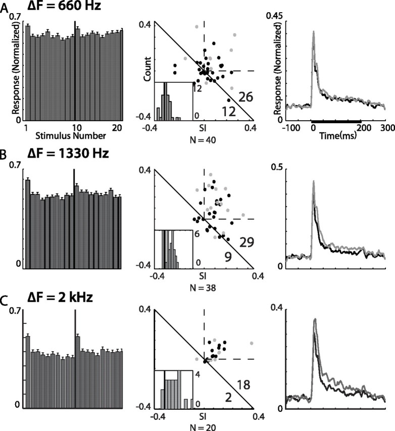
Summary of the results from frequency constant order tests in the OT. Results from tests with frequency gaps of 660, 1330, and 2000 Hz are shown in A, B, and C respectively. Histograms in the left column show the population response (normalized and averaged across all recording sites) to the constant order sequence of 20 stimuli. The first 10 bars present responses to the stimuli with the lower CF (relative to the best frequency) and the last 10 bars present responses to the higher CF. Error bars indicate SEs. The SIs scatterplots are shown in the middle column. The number of points above and below the diagonal line are shown in the bottom right corner. Gray points designate recordings from single units. Insets depict the NI distributions. The abscissa of the NI histogram is between −0.2 and 0.55 in all histograms. The right column shows the population PSTHs, normalized and averaged. Gray lines designate the population response to the rare stimulus and black lines designate the population response to the common stimulus. The bar in the top plot represents the duration of stimulation.
Figure 10.

Summary of results from ITD constant order tests in OT. Results from constant order tests presented with an ITD gap of 20 μs are shown in A and results from tests with an ITD gap of 40 μs are shown in B. The format is as in Figure 8.
Figure 12.

Summary of results from ITD constant order tests in the ICX. A, Results from tests with ITD gaps of 20 μs. B, Results from tests with ITD gaps of 40 μs. Histograms in the left column show the population response (normalized and averaged across all recording sites) to the constant order sequence of 20 stimuli. The first 10 bars present responses to the stimuli with ITD values left of the best ITD and the last 10 bars present responses to ITD values right of the best ITD. Error bars indicate SEs. The NI distribution and the SIs scatterplots (insets) are shown in the middle column. The number of points above and below the diagonal line are shown in the top right and bottom left corners of the scatterplots, respectively. Right column shows the population PSTHs, normalized and averaged. Gray lines designate the population response to the rare stimulus and black lines designate the population response to the common stimulus. The bar in the top plot represents the duration of stimulation.
Figure 14.

Summary of SSA effects in the ICX (left), OT (center), and AGFs (right). The error bars represent the average NI measured for frequency gaps of 2 kHz, ITD gaps of 40 μs, ABSI gaps of 30 dB, and ILD gaps of 15 dB. Error bars indicate the SE. Asterisks denote a significant deviation from zero (one-tailed, t test, p < 0.001; for all other cases p > 0.05).
Results
SSA in the AGFs
SSA was studied using the oddball stimulus paradigm (see Materials and Methods). An example of one recording site in the AGFs is shown in Figure 3. Here, a sequence of 150 sound stimuli was presented from which the ITD value of 127 randomly selected stimuli was −80 μs in block 1 and −100 μs in block 2 (frequent presentations). The remaining 23 stimuli had ITD values of −100 and −80 μs in blocks 1 and 2, respectively (rare presentations). Both ITD values were within the response range of the recorded site, eliciting significant responses. The average response for an ITD of −80 μs was slightly larger than for −100 μs (Fig. 3B). Nevertheless, for both ITDs, the average response to the rare presentation was significantly stronger than the response to the same ITD when frequent (Fig. 3A,B) (one-tailed t test, p < 0.001 for both stimuli). Note that it is not only the average spike rate that is larger in responses to rare stimuli, but also the response profile is different, as can be seen in the poststimulus time histogram in Figure 3, C and D. For example, an inhibitory window, which is apparent in the common responses (Fig. 3D, black line, arrow), is absent in the rare responses (Fig. 3D, gray line). The slight differences between the spontaneous firing rates of the rare and common responses, which can be seen in Figure 3, C and D (see also Fig. 5C,D), are caused by small fluctuations in the baseline activity that occurred on a time scale of several minutes. In most cases (97%), these differences did not reach a significant level (t test, p < 0.05).
Figure 3.

Example of a single AGF site response to an ITD oddball stimulus. A, Dot raster showing 40 responses to stimulus 1 (ITD, −80 μs). The bottom 20 rows show responses to the rarely presented sound (embedded in a sequence of sounds with an ITD of −100 μs). The top 20 rows show randomly picked responses to the same sound presented frequently. B, The average response to stimulus 1 and stimulus 2 when common (black bars) are compared with the average response to the same stimuli when rare (gray bars). Error bars represent SE. C, D, Poststimulus time responses to stimulus 1 (C) and to stimulus 2 (D) are shown (lines are smoothed for display). Gray lines designate responses to the rare presentation; black lines designate responses to the common presentation. The shaded area indicates the onset and duration of sound stimulation. The arrowhead in D points to an inhibitory window not visible in the average response to rare stimuli.
Figure 5.

Example of a single AGF site response to a frequency oddball test. A, Dot raster showing 40 responses to stimulus 1 (CF, 2 kHz). The bottom 20 rows show responses to the rarely presented sound (embedded in a sequence of sounds with a CF of 4 kHz). The top 20 rows show randomly picked responses to the same sound (CF, 2 kHz) frequently presented. B, The average response to stimulus 1 and stimulus 2 when common (black bars) are compared with the average response to the same stimuli when rare (gray bars). Error bars represent SE. C, D, Poststimulus time responses to stimulus 1 (C) and to stimulus 2 (D) are shown (lines are smoothed for display). Gray lines designate responses to the rare presentation; black lines designate responses to the frequent presentation. The shaded area indicates the onset and duration of sound stimulation.
A summary of the results from all sites (n = 43) measured in the AGFs is shown in Figure 4. For each test, two SIs and a single NI were calculated (see Materials and Methods). Tests were divided into three categories according to the difference between ITD values of the two stimuli: smaller than 30 μs (Fig. 4A), between 40 and 60 μs (Fig. 4B), and larger than 60 μs (Fig. 4C). The left column in Figure 4 presents the scatterplots of SI1 versus SI2 for all tests. A point appearing in the first quadrant (within the two dotted lines) implies stronger responses to the rare appearance of both stimuli. However, as pointed by Ulanovsky et al. (2003), any point above the diagonal line implies SSA: if the response to stimulus 1 when rare is stronger than the response to the same stimulus when common (SI1 > 0) and the adaptation is only activity dependent, it is expected that the response to stimulus 2 when rare will be smaller than when common (SI2 < 0) by an amount that is equal to SI1 (i.e., the point is expected to be on the diagonal). In all three cases (Fig. 4 A–C), a large number of points were within the first quadrant and the majority of points were significantly above the diagonal lines (sign test; p < 0.005) indicating the widespread presence of SSA. The distributions of the neural indices for the different conditions are presented in the middle column of Figure 4. Evidently, a tendency to respond stronger to rare stimuli (positive NI) appeared in all three conditions (one-tailed t test, p < 0.0001). The averaged PSTH of the normalized responses to rare stimuli (Fig. 4, right column, gray line) is compared with the average PSTH of the responses to the frequent stimuli (black line). The preferred response to rare presentations was apparent in all cases. The difference between the average rare and common responses increased systematically with the increase in the gap between the ITD values of the two stimuli.
To examine whether SSA in the AGFs can be elicited by a different acoustic feature rather than ITD, we measured responses to frequency oddball stimulation. Here the stimulus was a narrow noise band (1 kHz bandwidth); stimulus 1 differed from stimulus 2 only by the center frequency (CF) (see Materials and Methods). A frequency gap of 2 kHz between the two center frequencies was used in these experiments. An example from a single recording site in the AGFs is shown in Figure 5. In this example, the center frequencies of stimulus 1 and 2 were 2 and 4 kHz, respectively. In both cases, the responses elicited by rarely presented stimuli were significantly larger than those elicited by common stimuli (Fig. 5A,B). This effect was most dramatic for a stimulus of 2 kHz in which a common stimulus induced an average inhibitory response followed by a late excitatory response whereas the rare stimulus induced a clear excitatory response throughout the duration of the stimulus (Fig. 5C).
The results from 40 sites tested for a center frequency gap of 2 kHz are summarized in Figure 6. Similarly to the ITD tests, the majority of sites were significantly above the diagonal line (sign test, p < 0.001) (Fig. 6A). The NIs distribution was positively biased (t test, p < 10−5) (Fig. 6B), and the population PSTH of responses to the rare stimuli was above the population PSTH of responses to the common stimuli (Fig. 6C). Thus, we conclude that SSA in the AGFs can be induced by frequency changes as well as by ITD changes. The best frequency of the population of neurons used in this analysis ranged between 3 and 8 kHz. Therefore, a difference of 2 kHz corresponded to a normalized frequency difference [defined as Δf = (f2 − f1)/(f2 × f1)1/2) of 0.71–0.25. We did not attempt smaller frequency differences in the AGFs.
The majority of the analyzed population of responses was obtained from multiunit recordings (Figs. 4, 6, black dots). Therefore, we analyzed and displayed single-unit data separately to verify that the SSA reported above is not a particular outcome of the multiunit recordings. Figure 7A shows the population average PSTHs of responses to rare and common frequencies recorded only from well isolated single units (see Materials and Methods) (n = 17). Figure 7B shows the single-unit responses to rare and common ITDs (n = 19). In both cases the average response to rare stimuli was larger than the average response to common stimuli and the distribution of the NIs (insets) was positively biased (t test, p < 10−4). The stimulus indices calculated from these single units (Figs. 4, 6, left column, gray dots) were evenly distributed among the multiunit data (black dots). Thus, we conclude that SSA in the AGFs is expressed in single as well as multiunit recordings. Recordings from single units in the OT (n = 13) yielded a similar agreement between multiunit and single-unit data (data not shown).
SSA in the OT
Next we characterized the responses of neurons in the OT to the oddball stimulus, testing either frequency or ITD changes. The scatterplots of SI1 versus SI2, obtained from all recording sites in the OT where an oddball ITD test was performed (n = 74) and from all sites in the OT where an oddball frequency test was performed (n = 29), are shown in Figure 8, A and B, respectively. Both these acoustic features gave rise to SSA effects in the majority of neurons (sign test, p < 10−4). Thus, we conclude that SSA of ITD and of frequency is expressed in the neural responses of tectal neurons, as was shown in AGF neurons (Figs. 4, 6).
Figure 8.

Summary of results from oddball tests in the OT. A, Scatterplot of SI1 versus SI2. of ITD oddball tests with 20–40 μs gaps between the ITD of stimulus 1 and stimulus 2. B, Scatterplot of SI1 versus SI2 obtained from frequency oddball tests with a 2 kHz gap between the center frequency of stimulus 1 and stimulus 2. The number of points above and below the diagonal line are shown in the bottom right corner. The dashed lines mark the first quadrant where both SIs are positive. All points represent multiunit recordings. The insets show the population average response to the stimulus that directly preceded a rare event (left bar) and to the first and second stimuli that immediately followed a rare event (middle bar and right bar, respectively). The gap in the histograms represents the position of the rare event in the sequence. The error bars designate the SE.
The appearance of a rare stimulus in the oddball design is probabilistic, resembling the arrival of stimuli in nature. It is possible that this feature of the oddball design is essential to elicit the SSA effects recorded above. To test this hypothesis we used a CO stimulation design (see Materials and Methods) (Fig. 2B) as opposed to the stochastic oddball stimulus. The results of the CO frequency tests in the OT are summarized in Figure 9. CF values of the two stimuli were separated by a gap of either 660 Hz (Fig. 9A), 1330 Hz (Fig. 9B), or 2000 Hz (Fig. 9C). The bandwidth of the stimuli was maintained at 1 kHz, implying a substantial overlap between the frequency bands at the small gap of 660 Hz. For frequency gaps of 2000 Hz and 1330 Hz, the average response to the first stimulus in a sequence of 10 identical stimuli was significantly stronger than the average response to the last stimulus in the sequence (t test, p < 0.05) (Fig. 9B,C), indicating the tendency of tectal neurons to specifically adapt to the stimulus frequency. A frequency gap of 660 Hz did not achieve a significant difference. Note the rapid adaptation in all three conditions, reaching approximately the steady-state level after one novel stimulus (Fig. 9, left column).
To compare the time course of adaptation with that presented in the probabilistic stimulation we normalized and averaged the neural responses to three groups of stimuli in the oddball test: (1) frequent stimuli that directly preceded a rare event and (2, 3) the two consecutive frequent stimuli that immediately followed a rare event. The average response to the first stimulus after a single display of a rare ITD (Fig. 8A, inset) or a rare frequency (Fig. 8B, inset) was significantly stronger than the average response to the subsequent stimulus (second stimulus after the rare event; t test, p < 0.01). The average response to this second stimulus, however, in both ITD and frequency tests was not significantly different from the average response to the stimulus directly preceding a rare event. These results suggest that the adaptation occurred on a fast time scale, similar to the adaptation observed in the constant order tests, and that a single different event in the sequence was sufficient to initiate a recovery from SSA. The degree of the effect was substantially smaller than in the constant order tests (Figs. 9, 10), where the recovery was initiated by a sequence of 10 preceding events.
To quantify the size of the SSA effect, we calculated two indices similar to the oddball paradigm (see Materials and Methods). Scatterplots of the SIs (Fig. 9, center column) and histograms of the NIs (inset) were consistent with response averages – the two larger frequency gaps obtained an NI distribution significantly shifted toward positive values (t test, p < 0.01 and p < 0.001 for 1330 Hz and 2000 Hz, respectively), whereas a frequency difference of 660 Hz did not achieve a significant deviation from zero. It is evident from the PSTHs depicted in the right column that the difference between the responses to frequent and rare stimuli increased systematically with the increase in frequency gap.
Figure 10 shows the results from the experiments in which only the ITD value was interchanged between the two parts of the frozen sequence. The ITD gap was either 20 μs (Fig. 10A) or 40 μs (Fig. 10B). It can be seen that the average response to the first stimulus in a sequence was significantly stronger than the average response to the last stimulus (t test, p < 0.0005). This result is also demonstrated by the positive distribution of the neural indices (t test, p < 0.00005) (Fig. 10, middle column) and by the differences in the average response profiles shown in Figure 10 (right column). Both 20 and 40 μs disparities elicited stronger average responses to rare stimuli. Similar to the frequency domain, a tendency for a stronger SSA effect with increased ITD disparity was apparent. In summary, we did not observe any qualitative differences between the adaptation in the oddball design and the adaptation in the CO design. In the following further characterization of SSA in the midbrain pathway, we used the CO design exclusively.
SSA of ITD and frequency in the ICX
To track the origin of the SSA that appeared in the OT, we recorded from the primary source of auditory input to the OT, the ICX (Knudsen and Knudsen, 1983). Stimulus-specific adaptation to frequency was evident in ICX neurons (Fig. 11). All three frequency gaps tested revealed a significant difference between the average response to the first stimulus compared with the average response to the last stimulus (t test, p < 0.05, 0.01, and 0.001 for frequency difference of 660, 1330, and 2000 Hz, respectively). Similar to the results obtained in the OT, SSA effects were larger for wider frequency gaps (Fig. 11B). Thus, frequency-specific adaptation in the OT can largely be explained by adaptation occurring at earlier stations along the pathway. This, however, was not the case for ITD-specific adaptation. In the sampled group of neurons from the ICX (Fig. 12), no ITD SSA effect was observed as is indicated by the constant average response (Fig. 12, left column), by the distribution of neuron indices, which was not significantly different from zero (Fig. 12, middle column) (p > 0.05), and by the overlapping average PSTHs (Fig. 12, right column). The lack of ITD SSA in the ICX was apparent even when increasing the gap between the ITD values of the two stimuli from 20 μs (Fig. 12A) to 40 μs (Fig. 12B). Results acquired in the ICX using the oddball paradigm (data not shown) agreed with the above results, namely ITD SSA was not visible in the ICX.
Figure 11.

Summary of results from frequency constant order tests in the ICX. A, The population response (normalized and averaged) to the constant order sequence with a frequency gap of 2 kHz. The first 10 bars present responses to the stimuli with the lower CF (relative to the best frequency) and the last 10 bars present responses to the higher CF. Error bars indicate SE. B, The NIs are shown versus the frequency gap used in the test. The line connects the average points at each frequency gap.
SSA of sound intensity and ILD in the midbrain
If SSA in the OT is a basis for novelty detection, we would expect that the phenomenon will be manifested in a wide range of acoustic features. To test this hypothesis we characterized the generality of SSA in the midbrain by testing the CO stimulus design with yet two additional acoustic features: the ABSI and the ILD. In the first test (Fig. 13A), the two stimuli differed only in the ABSI. The left side of the bar chart in Figure 13A shows the average responses to the weak stimulus (10–15 dB above threshold), whereas the right side of the histogram shows the average responses to the loud stimulus (30 dB above the weak stimulus). The average response to the first stimulus in a block was significantly stronger than the response to the last stimulus for both loud and weak sounds (Fig. 13A,C) (t test, p < 10−6), and the distribution of the neural indices was significantly biased to positive values (Fig. 13B) (t test p < 10−8). Thus, tectal neurons undergo specific adaptation to the intensity of the sound. Interestingly, this result was not visible in neurons from the ICX. The mean NI was not significantly different from zero, and the responses to the first sound in a sequence of 10 identical stimuli were not significantly different from the responses to the last sound in the sequence (Fig. 13 D–F). Therefore, ABSI SSA appeared in the OT and not in the ICX.
Figure 13.

Results of additional acoustic features in the OT and ICX. A, Population average response to a constant order sequence. The first 10 bars show the average responses to a sequence of sounds with low ABSI, the second 10 bars show the responses to a sequence of sounds with a higher ABSI (30 dB relative to the ABSI of the low sound). B, Scatterplot of SI1 versus SI2 of the same neurons as in A. The gray points designate recordings from single units. The inset shows the distribution of the NIs. The abscissa of the NI histogram is between −0.2 and 0.55 in all histograms. C, The population PSTHs, normalized and averaged, are shown for the rare stimulus (gray line) and for the frequent stimulus (black line). The responses to the low-intensity sound and to the high-intensity sound are shown separately in the top and bottom plots, respectively. D–F, Results from neurons in the ICX tested under the same stimulus conditions as in A–C. D, The population response to the constant order sequence. E, NI distribution and scatterplot of SIs. F, Population PSTH responses to rare (gray line) and frequent (black line) sound intensities. Responses to both low and high intensities are averaged together. G, Population response to a constant order sequence in which the ILD of the first 10 stimuli differed by 15 dB (toward contra lateral ear louder) from the ILD displayed in the second 10 stimuli. H, The scatterplot of SIs and the distribution of the NIs of all ILD tests. The gray points designate recordings from single units. I, The average response to rare (gray line) and frequent (black line) stimulus are shown separately for the louder contralateral ear (top plot) and the louder ipsilateral ear (bottom plot). J–L, Results from neurons in the ICX under the same stimulus conditions as in G–I.
In the second test, the two stimuli differed only in ILD. The results of this test were qualitatively similar to the results obtained for ABSI and ITD tests, namely an SSA effect was evident in the OT and not in the preceding auditory station, the ICX. The average response to the first stimulus in a block was significantly stronger than the response to the last stimulus for both contralateral-ear-leading and ipsilateral-ear-leading sounds (Fig. 13G,I) (t test, p < 0.005), and both NIs and SIs were significantly biased toward positive values (Fig. 13H) (t test, p < 10−5; sign test, p < 10−4). In the ICX, however, rare and frequent stimuli elicited identical responses and the mean NI was not significantly different from zero (Fig. 13 J–L).
A summary of the mean NIs measured in the three different brain structures (OT, ICX, and AGFs) is shown in Figure 14. In the OT, all four acoustic features (ITD, ILD, ABSI, and frequency) elicited significant SSAs. At the same parameter gaps that elicited clear SSAs in the OT, SSAs were not present in the ICX. Frequency was an exceptional feature: only SSA for frequency was manifested both in the OT and the ICX. In the forebrain AGFs, both ITD and frequency elicited SSAs. We did not test for ABSI or ILD SSAs in the forebrain.
A close look at the onsets of the average responses permits the inspection of the relative population delays of responses to rare versus common stimuli. Figure 15A shows the onsets (first 40 ms) of the population average responses in the OT for ABSI, frequency, ILD, and ITD tests. The bottom gray line is the difference between the responses to rare (top gray line) and common (black line) stimuli. All curves were smoothed with a sliding average window of 6 ms. The time of onset was estimated as the point where the curve crossed the threshold, defined as 30% of the peak plus 1.5 times the SD of the spontaneous activity. It is evident that for all four acoustic parameters tested, the average population responses to the rare and to the common stimuli initially overlapped. The difference between the responses initiated several ms after the onset of the population responses (Fig. 15A, compare gray and black ticks). This short delay in the initiation of the difference may reflect a circumstance where SSA occurs only in a subpopulation of neurons in the OT with long response latencies. To check this possibility, we correlated the response latency with the SI for each stimulus condition. In all conditions the SI did not increase significantly with the response latency of the neurons (ANOVA F test, p > 0.05). Three examples are shown in Figure 15B: the 2 kHz frequency gap, 40 μs ITD gap, and 30 dB ABSI gap. Our results suggest that the enhancing effect of SSA is not initiated together with response onset, but shortly afterward (∼5 ms).
Figure 15.

The onset of SSA effect in the OT. A, A close look at the time window starting 5 ms before and ending 40 ms after the onset of the stimulus is shown for the PSTHs from Figures 13C (ABSI, 30 dB gap), 9C (frequency, 2 kHz gap), 13I (ILD, 15 dB gap), and 10B (ITD, 40 μs gap). The top gray line shows the response to a rarely presented stimulus, the black line shows the response to a frequently presented stimulus, and the bottom gray line shows the difference between the two. The arrowheads indicate the stimulus onset. The black ticks present the latency of the population response to the frequent stimulus and the gray ticks present the latency of the difference signal. B, The stimulus indices versus the latencies to response are shown for frequency tests (top plot), ITD tests (middle plot), and ABSI tests (bottom plot). The horizontal lines designate the zero axes.
Discussion
Stimulus-specific adaptation in the auditory system
Adaptation is a ubiquitous property of neurons in the auditory system. Most types of adaptations described in the literature depend on the activation history of the neuron more than on specific features of the stimulus (Calford and Semple, 1995; Brosch and Schreiner, 1997; McAlpine et al., 2000; Ingham and McAlpine, 2004; Furukawa et al., 2005; Wehr and Zador, 2005; Gutfreund and Knudsen, 2006). A different, higher-level adaptation is SSA, an adaptation to the history of the stimulus rather than to the activity of the neuron (Ulanovsky et al., 2003, 2004). Neurons that adapt to specific features of the stimulus integrate sensory information to create a model of the world, responding stronger to novel features in the environment. The computations to achieve such stimulus-specific responses require a network to compare between current and past stimulus conditions (Abbott et al., 1997; Eytan et al., 2003).
In the auditory system, SSA has been described in the auditory cortex (Ulanovsky et al., 2003, 2004) and in the inferior colliculus (IC) (Malone and Semple, 2001). However, the stimulus protocol used to elicit SSA in the cortex and in the IC differed substantially, obscuring direct comparison between the two phenomena. Moreover, Malone and Semple (2001) showed that the auditory response of many neurons in the IC cannot be predicted simply by the cell's discharge history. This, however, does not necessarily imply SSA as defined here because the adaptation may be determined by processes other than discharge rates (e.g., spike timing, subthreshold activity, etc.). The stimulus protocol and analysis used by Ulanovsky et al. (2003) avoids this difficulty by using bidirectional comparison; adaptation is considered specific to the stimulus if the responses to both stimulus 1 and 2, when rare, are stronger than the responses to the same stimuli when common, a state that cannot be achieved if the activity alone determines the adaptation. Here we used the same analysis used by Ulanovsky et al. (2003) to measure SSA directly. The adaptation we report in the OT and AGFs resembles the SSA in the auditory cortex in several aspects: in the cortex, adaptation develops over a time scale of seconds, comparable with the time scale we report here (Figs. 9–11, 13). Moreover, in the cortex the adaptation is extremely specific to the frequency of the stimulus; a very small frequency gap, compared with the tuning width of the neurons, was sufficient to induce a significant SSA. In the present work, although we did not systematically check the level of specificity, we show that ITD gaps of 20 μs, which are finer than the response range of typical neurons in the OT, elicited SSA effects (Fig. 10A). Another striking similarity is the abrupt appearance of SSA in the pathway. Neurons in the medial geniculate nucleus, which provide inputs to the auditory cortex, did not exhibit SSA (Ulanovsky et al., 2003). Similarly, neurons in the ICX, the source of auditory information to the OT, did not show SSA for ITD, ILD and ABSI (Figs. 12, 13). An exception to this was the frequency SSA, which was observed in ICX neurons. Interestingly, SSA to frequency was recently reported in a sub population of IC neurons in rats (Perez-Gonzalez et al., 2005).
Implication of SSA in the localization pathway
The SSA in the OT was found to be relatively invariant to the feature tested: in all cases (ITD, ILD, ABSI, and frequency) the adaptation was stimulus specific, developed rapidly (1 trial) (Figs. 9, 10, 13) and the adaptation memory was at least 1 s long (we did not attempt other ISIs). This similarity is especially striking taking into account that the four features are represented and computed in marginally different ways: ITD and ILD, the two primary binaural localization cues, are processed in parallel in two separate and independent brainstem pathways that converge in the lateral shell of the central nucleus of the inferior colliculus (ICCls) (Takahashi et al., 1984; Takahashi and Konishi, 1988; Adolphs, 1993; Albeck and Konishi, 1995) to induce selectivity to spatial locations, which is then further refined along the pathway to the ICX and on to the OT (Moiseff and Konishi, 1983; Pena and Konishi, 2001). Frequency separation is maintained in both ascending auditory pathways from the cochlea up to the level of the ICCls where information across frequency-specific channels is combined (Euston and Takahashi, 2002). Sound-level information is presumably manifested in the response levels of the ascending pathways. The fact that all four independent acoustic features showed a qualitatively similar pattern of adaptation suggests that SSA is an important property in the neural representation of the auditory scene. Possibly, this property underlies the owl's ability to attend and orient abruptly to novel events. We hypothesize that similar auditory SSA exists in the superior colliculus of mammalian species. However, to our knowledge this has not been studied. Interestingly, we also found strong spatial SSA in the OT for visual stimuli (data not shown), suggesting that SSA in the OT is a multisensory phenomenon.
Mechanisms of SSA
Several types of adaptation mechanisms have been described, including synaptic depression (Wehr and Zador, 2005), delayed inhibition (Schmidt and Perkel, 1998; Tan et al., 2004; Wehr and Zador, 2005), and intrinsic cellular properties such as voltage- or calcium-dependent potassium currents (Gollisch and Herz, 2004). Any mechanism of adaptation can be involved in generating SSA provided that the two stimuli activate separate paths to the recorded neuron and that the adaptation acts at a level where the activation is significantly separated (Eytan et al., 2003). Previous studies in barn owls have reported adaptation effects in the afferent auditory pathway to the OT (Wagner et al., 2002; Spitzer et al., 2004; Gutfreund and Knudsen, 2006). However, in all of these cases, the adaptation was relatively short lasting, incapable of accounting for the 1 s ISI used in the current study.
A key observation in this work was the qualitative difference between the OT and its main source of auditory input, calling for at least two separate sites of adaptation to account for the SSA effects. Adaptation acting at frequency-specific lower levels of the auditory pathway could explain frequency SSA but is unlikely to explain ITD, ILD, or ABSI SSA. One possibility is that the adaptation mechanism of the latter is a short term synaptic depression acting at ICX-OT synapses, similar to depression at thalamocortical synapses proposed to underlie SSA in the cortex (Katz et al., 2006). However, the observation shown in Figure 15 that the SSA in the OT, on average, tends to develop several milliseconds after the onset of response suggests that the SSA is happening not at the direct pathway to the tectal neurons, but involves an additional level of processing either internal in the OT or external arriving from other parts of the brain.
Origin of SSA
Among the indirect pathways to the OT, the extensively studied isthmotectal loop has been suggested to be involved in spatial attention (Marin et al., 2005). Nucleus isthmi, the homolog of the mammalian nucleus parabigeminalis (Diamond et al., 1992), receives auditory and visual afferents from tectal neurons, and send cholinergic projections back to the tectum (Maczko et al., 2006). This may constitute a winner-take-all network that enhances the sensitivity of tectal neurons to the location of the most salient stimulus (Marin et al., 2005; Wang et al., 2006; Knudsen, 2007). Adaptation in the isthmotectal loop has not been reported so far. In principle, because of the high spatial precision, such adaptation may induce tectal SSA in ITD and ILD, two cues that are topographically represented in the OT. This mechanism, however, cannot account for SSA of nonspatial parameters such as intensity.
An additional indirect auditory pathway to the OT is conveyed through the AGFs (Cohen et al., 1998). This forebrain nucleus has been shown to be involved in auditory working memory (Knudsen and Knudsen, 1996a), a vital feature for specific adaptation of the time scales presented here. Moreover, a recent study has shown that focal electrical microstimulation in the AGFs enhances tectal auditory responses in a space-specific manner (Winkowski and Knudsen, 2006). Such top-down effects have been suggested to be involved in control of spatial attention in mammals and birds (Moore and Fallah, 2004; Winkowski and Knudsen, 2006). These findings raise the possibility that SSA originates in forebrain networks, giving rise to top-down signals that enhance responses to rare stimuli in the OT. In agreement with this model, a similar stimulation paradigm used in the OT revealed frequency and ITD SSA in the AGFs (Figs. 3–6). Interestingly, the AGFs project to the isthmi pars parvocellularis (Knudsen et al., 1995), a connection that may enable forebrain control of tectal sensitivity through the isthmotectal system. The involvement of the forebrain and nucleus isthmi in the generation of SSA is yet to be validated in future experimental work.
Footnotes
This work was supported by a Bikura grant from the Israel Science Foundation and by the Joel Elkes grant from the National Psychobiology Institute in Israel (founded by the E. Smith family). We thank Prof. Eli Nelken for advice and careful reading of this manuscript and Felix Milman for technical support.
References
- Abbott LF, Varela JA, Sen K, Nelson SB. Synaptic depression and cortical gain control. Science. 1997;275:220–224. doi: 10.1126/science.275.5297.221. [DOI] [PubMed] [Google Scholar]
- Adolphs R. Bilateral inhibition generates neuronal responses tuned to interaural level differences in the auditory brainstem of the barn owl. J Neurosci. 1993;13:3647–3668. doi: 10.1523/JNEUROSCI.13-09-03647.1993. [DOI] [PMC free article] [PubMed] [Google Scholar]
- Albeck Y, Konishi M. Responses of neurons in the auditory pathway of the barn owl to partially correlated binaural signals. J Neurophysiol. 1995;74:1689–1700. doi: 10.1152/jn.1995.74.4.1689. [DOI] [PubMed] [Google Scholar]
- Bala AD, Takahashi TT. Pupillary dilation response as an indicator of auditory discrimination in the barn owl. J Comp Physiol [A] 2000;186:425–434. doi: 10.1007/s003590050442. [DOI] [PubMed] [Google Scholar]
- Brainard MS, Knudsen EI. Experience-dependent plasticity in the inferior colliculus: a site for visual calibration of the neural representation of auditory space in the barn owl. J Neurosci. 1993;13:4589–4608. doi: 10.1523/JNEUROSCI.13-11-04589.1993. [DOI] [PMC free article] [PubMed] [Google Scholar]
- Brosch M, Schreiner CE. Time course of forward masking tuning curves in cat primary auditory cortex. J Neurophysiol. 1997;77:923–943. doi: 10.1152/jn.1997.77.2.923. [DOI] [PubMed] [Google Scholar]
- Bruce CJ, Goldberg ME. Primate frontal eye fields. I. Single neurons discharging before saccades. J Neurophysiol. 1985;53:603–635. doi: 10.1152/jn.1985.53.3.603. [DOI] [PubMed] [Google Scholar]
- Calford MB, Semple MN. Monaural inhibition in cat auditory cortex. J Neurophysiol. 1995;73:1876–1891. doi: 10.1152/jn.1995.73.5.1876. [DOI] [PubMed] [Google Scholar]
- Cohen YE, Knudsen EI. Binaural tuning of auditory units in the forebrain archistriatal gaze fields of the barn owl: local organization but no space map. J Neurosci. 1995;15:5152–5168. doi: 10.1523/JNEUROSCI.15-07-05152.1995. [DOI] [PMC free article] [PubMed] [Google Scholar]
- Cohen YE, Miller GL, Knudsen EI. Forebrain pathway for auditory space processing in the barn owl. J Neurophysiol. 1998;79:891–902. doi: 10.1152/jn.1998.79.2.891. [DOI] [PubMed] [Google Scholar]
- Corbetta M. Frontoparietal cortical networks for directing attention and the eye to visual locations: identical, independent, or overlapping neural systems? Proc Natl Acad Sci USA. 1998;95:831–838. doi: 10.1073/pnas.95.3.831. [DOI] [PMC free article] [PubMed] [Google Scholar]
- Diamond IT, Fitzpatrick D, Conley M. A projection from the parabigeminal nucleus to the pulvinar nucleus in Galago. J Comp Neurol. 1992;316:375–382. doi: 10.1002/cne.903160308. [DOI] [PubMed] [Google Scholar]
- Diliberto KA, Altarriba J, Neill WT. Novel popout and familiar popout in a brightness discrimination task. Percept Psychophys. 2000;62:1494–1500. doi: 10.3758/bf03212149. [DOI] [PubMed] [Google Scholar]
- Euston DR, Takahashi TT. From spectrum to space: the contribution of level difference cues to spatial receptive fields in the barn owl inferior colliculus. J Neurosci. 2002;22:284–293. doi: 10.1523/JNEUROSCI.22-01-00284.2002. [DOI] [PMC free article] [PubMed] [Google Scholar]
- Eytan D, Brenner N, Marom S. Selective adaptation in networks of cortical neurons. J Neurosci. 2003;23:9349–9356. doi: 10.1523/JNEUROSCI.23-28-09349.2003. [DOI] [PMC free article] [PubMed] [Google Scholar]
- Furukawa S, Maki K, Kashino M, Riquimaroux H. Dependency of the interaural phase difference sensitivities of inferior collicular neurons on a preceding tone and its implications in neural population coding. J Neurophysiol. 2005;93:3313–3326. doi: 10.1152/jn.01219.2004. [DOI] [PubMed] [Google Scholar]
- Gold JI, Knudsen EI. A site of auditory experience-dependent plasticity in the neural representation of auditory space in the barn owl's inferior colliculus. J Neurosci. 2000;20:3469–3486. doi: 10.1523/JNEUROSCI.20-09-03469.2000. [DOI] [PMC free article] [PubMed] [Google Scholar]
- Gollisch T, Herz AV. Input-driven components of spike-frequency adaptation can be unmasked in vivo. J Neurosci. 2004;24:7435–7444. doi: 10.1523/JNEUROSCI.0398-04.2004. [DOI] [PMC free article] [PubMed] [Google Scholar]
- Gutfreund Y, Knudsen EI. Adaptation in the auditory space map of the barn owl. J Neurophysiol. 2006;17:17. doi: 10.1152/jn.01144.2005. [DOI] [PubMed] [Google Scholar]
- Hanes DP, Thompson KG, Schall JD. Relationship of presaccadic activity in frontal eye field and supplementary eye field to saccade initiation in macaque: poisson spike train analysis. Exp Brain Res. 1995;103:85–96. doi: 10.1007/BF00241967. [DOI] [PubMed] [Google Scholar]
- Ingham NJ, McAlpine D. Spike-frequency adaptation in the inferior colliculus. J Neurophysiol. 2004;91:632–645. doi: 10.1152/jn.00779.2003. [DOI] [PubMed] [Google Scholar]
- Katz Y, Heiss JE, Lampl I. Cross-whisker adaptation of neurons in the rat barrel cortex. J Neurosci. 2006;26:13363–13372. doi: 10.1523/JNEUROSCI.4056-06.2006. [DOI] [PMC free article] [PubMed] [Google Scholar]
- Knudsen EI. Auditory and visual maps of space in the optic tectum of the owl. J Neurosci. 1982;2:1177–1194. doi: 10.1523/JNEUROSCI.02-09-01177.1982. [DOI] [PMC free article] [PubMed] [Google Scholar]
- Knudsen EI. Fundamental components of attention [review] Annu Rev Neurosci. 2007;30:57–78. doi: 10.1146/annurev.neuro.30.051606.094256. [DOI] [PubMed] [Google Scholar]
- Knudsen EI, Knudsen PF. Space-mapped auditory projections from the inferior colliculus to the optic tectum in the barn owl (Tyto alba) J Comp Neurol. 1983;218:187–196. doi: 10.1002/cne.902180206. [DOI] [PubMed] [Google Scholar]
- Knudsen EI, Knudsen PF. Disruption of auditory spatial working memory by inactivation of the forebrain archistriatum in barn owls. Nature. 1996a;383:428–431. doi: 10.1038/383428a0. [DOI] [PubMed] [Google Scholar]
- Knudsen EI, Knudsen PF. Contribution of the forebrain archistriatal gaze fields to auditory orienting behavior in the barn owl. Exp Brain Res. 1996b;108:23–32. doi: 10.1007/BF00242901. [DOI] [PubMed] [Google Scholar]
- Knudsen EI, Cohen YE, Masino T. Characterization of a forebrain gaze field in the archistriatum of the barn owl: microstimulation and anatomical connections. J Neurosci. 1995;15:5139–5151. doi: 10.1523/JNEUROSCI.15-07-05139.1995. [DOI] [PMC free article] [PubMed] [Google Scholar]
- Maczko KA, Knudsen PF, Knudsen EI. Auditory and visual space maps in the cholinergic nucleus isthmi pars parvocellularis of the barn owl. J Neurosci. 2006;26:12799–12806. doi: 10.1523/JNEUROSCI.3946-06.2006. [DOI] [PMC free article] [PubMed] [Google Scholar]
- Malone BJ, Semple MN. Effects of auditory stimulus context on the representation of frequency in the gerbil inferior colliculus. J Neurophysiol. 2001;86:1113–1130. doi: 10.1152/jn.2001.86.3.1113. [DOI] [PubMed] [Google Scholar]
- Marin G, Mpodozis J, Sentis E, Ossandon T, Letelier JC. Oscillatory bursts in the optic tectum of birds represent re-entrant signals from the nucleus isthmi pars parvocellularis. J Neurosci. 2005;25:7081–7089. doi: 10.1523/JNEUROSCI.1379-05.2005. [DOI] [PMC free article] [PubMed] [Google Scholar]
- McAlpine D, Jiang D, Shackleton TM, Palmer AR. Responses of neurons in the inferior colliculus to dynamic interaural phase cues: evidence for a mechanism of binaural adaptation. J Neurophysiol. 2000;83:1356–1365. doi: 10.1152/jn.2000.83.3.1356. [DOI] [PubMed] [Google Scholar]
- Moiseff A, Konishi M. Binaural characteristics of units in the owl's brainstem auditory pathway: precursors of restricted spatial receptive fields. J Neurosci. 1983;3:2553–2562. doi: 10.1523/JNEUROSCI.03-12-02553.1983. [DOI] [PMC free article] [PubMed] [Google Scholar]
- Moore T, Fallah M. Microstimulation of the frontal eye field and its effects on covert spatial attention. J Neurophysiol. 2004;91:152–162. doi: 10.1152/jn.00741.2002. [DOI] [PubMed] [Google Scholar]
- Moore T, Armstrong KM, Fallah M. Visuomotor origins of covert spatial attention. Neuron. 2003;40:671–683. doi: 10.1016/s0896-6273(03)00716-5. [DOI] [PubMed] [Google Scholar]
- Nelken I. Processing of complex stimuli and natural scenes in the auditory cortex. Curr Opin Neurobiol. 2004;14:474–480. doi: 10.1016/j.conb.2004.06.005. [DOI] [PubMed] [Google Scholar]
- Pena JL, Konishi M. Auditory spatial receptive fields created by multiplication. Science. 2001;292:249–252. doi: 10.1126/science.1059201. [DOI] [PubMed] [Google Scholar]
- Perez-Gonzalez D, Malmierca MS, Covey E. Novelty detector neurons in the mammalian auditory midbrain. Eur J Neurosci. 2005;22:2879–2885. doi: 10.1111/j.1460-9568.2005.04472.x. [DOI] [PubMed] [Google Scholar]
- Ranganath C, Rainer G. Neural mechanisms for detecting and remembering novel events. Nat Rev Neurosci. 2003;4:193–202. doi: 10.1038/nrn1052. [DOI] [PubMed] [Google Scholar]
- Schmidt MF, Perkel DJ. Slow synaptic inhibition in nucleus HVc of the adult zebra finch. J Neurosci. 1998;18:895–904. doi: 10.1523/JNEUROSCI.18-03-00895.1998. [DOI] [PMC free article] [PubMed] [Google Scholar]
- Sobotka S, Ringo JL. Stimulus specific adaptation in excited but not in inhibited cells in inferotemporal cortex of macaque. Brain Res. 1994;646:95–99. doi: 10.1016/0006-8993(94)90061-2. [DOI] [PubMed] [Google Scholar]
- Sparks DL. Translation of sensory signals into commands for control of saccadic eye movements: role of primate superior colliculus. Physiol Rev. 1986;66:118–171. doi: 10.1152/physrev.1986.66.1.118. [DOI] [PubMed] [Google Scholar]
- Spitzer MW, Bala AD, Takahashi TT. A neuronal correlate of the precedence effect is associated with spatial selectivity in the barn owl's auditory midbrain. J Neurophysiol. 2004;92:2051–2070. doi: 10.1152/jn.01235.2003. [DOI] [PubMed] [Google Scholar]
- Takahashi T, Moiseff A, Konishi M. Time and intensity cues are processed independently in the auditory system of the owl. J Neurosci. 1984;4:1781–1786. doi: 10.1523/JNEUROSCI.04-07-01781.1984. [DOI] [PMC free article] [PubMed] [Google Scholar]
- Takahashi TT, Konishi M. Projections of the cochlear nuclei and nucleus laminaris to the inferior colliculus of the barn owl. J Comp Neurol. 1988;274:190–211. doi: 10.1002/cne.902740206. [DOI] [PubMed] [Google Scholar]
- Tan AY, Zhang LI, Merzenich MM, Schreiner CE. Tone-evoked excitatory and inhibitory synaptic conductances of primary auditory cortex neurons. J Neurophysiol. 2004;92:630–643. doi: 10.1152/jn.01020.2003. [DOI] [PubMed] [Google Scholar]
- Tiitinen H, May P, Reinikainen K, Naatanen R. Attentive novelty detection in humans is governed by pre-attentive sensory memory. Nature. 1994;372:90–92. doi: 10.1038/372090a0. [DOI] [PubMed] [Google Scholar]
- Ulanovsky N, Las L, Nelken I. Processing of low-probability sounds by cortical neurons. Nat Neurosci. 2003;6:391–398. doi: 10.1038/nn1032. [DOI] [PubMed] [Google Scholar]
- Ulanovsky N, Las L, Farkas D, Nelken I. Multiple time scales of adaptation in auditory cortex neurons. J Neurosci. 2004;24:10440–10453. doi: 10.1523/JNEUROSCI.1905-04.2004. [DOI] [PMC free article] [PubMed] [Google Scholar]
- Wagner H. Sound-localization deficits induced by lesions in the barn owl's auditory space map. J Neurosci. 1993;13:371–386. doi: 10.1523/JNEUROSCI.13-01-00371.1993. Erratum (1993) 13. [DOI] [PMC free article] [PubMed] [Google Scholar]
- Wagner H, Mazer JA, von Campenhausen M. Response properties of neurons in the core of the central nucleus of the inferior colliculus of the barn owl. Eur J Neurosci. 2002;15:1343–1352. doi: 10.1046/j.1460-9568.2002.01970.x. [DOI] [PubMed] [Google Scholar]
- Wang Y, Luksch H, Brecha NC, Karten HJ. Columnar projections from the cholinergic nucleus isthmi to the optic tectum in chicks (Gallus gallus): a possible substrate for synchronizing tectal channels. J Comp Neurol. 2006;494:7–35. doi: 10.1002/cne.20821. [DOI] [PubMed] [Google Scholar]
- Wehr M, Zador AM. Synaptic mechanisms of forward suppression in rat auditory cortex. Neuron. 2005;47:437–445. doi: 10.1016/j.neuron.2005.06.009. [DOI] [PubMed] [Google Scholar]
- Weisbard C, Graham PK. Heart-rate change as a component of the orienting response in monkeys. J Comp Physiol Psychol. 1971;76:74–83. doi: 10.1037/h0031048. [DOI] [PubMed] [Google Scholar]
- Winkowski DE, Knudsen EI. Top-down gain control of the auditory space map by gaze control circuitry in the barn owl. Nature. 2006;439:336–339. doi: 10.1038/nature04411. [DOI] [PMC free article] [PubMed] [Google Scholar]