

Abstract
The timing of an upcoming event depends on two factors: its temporal position, proximal or distal with respect to the present moment, and the unavoidable stochastic variability around this temporal position. We searched for a general mechanism that could describe how these two factors influence the anticipation of an upcoming event in an oculomotor task. Monkeys were trained to pursue a moving target with their eyes. During a delay period inserted before target motion onset, anticipatory pursuit responses were frequently observed. We found that anticipatory movements were altered by the temporal position of the target. Increasing the timing uncertainty associated with the stimulus resulted in an increase in the width of the latency distribution of anticipatory pursuit. These results show that monkeys relied on an estimation of the changing probability of target motion onset as time elapsed during the delay to decide when to initiate an anticipatory smooth eye movement.
Keywords: eye movement, macaque, oculomotor, psychophysics, smooth pursuit, temporal coding
Introduction
In a rapidly changing visual environment, the delay between perception and action might impair the probability of survival of a prey or the efficiency of a predator. To compensate for this delay, primates make anticipatory movements that begin before the occurrence of a likely event. However, primates must decide and act knowing that the position of an event on the timeline can be near the present moment or further in the future and that the timing of an expected event is always uncertain.
To prepare a motor response to an expected event, an estimation of the conditional probability that the event will occur given that it has not occurred yet is necessary. This conditional probability is often termed the hazard function or hazard rate and continuously changes as time elapses before an expected event (Barlow et al., 1966; Luce, 1986; Grimmet and Stirzaker, 2005). In a visual detection task, it has been shown that the hazard rate could be used to guide the allocation of attention in the time domain (Ghose and Maunsell, 2002). Moreover, it has been shown that a subjective estimate of the hazard rate could describe the behavioral consequence of the anticipation of a “go” signal in a saccade task and could be represented in the LIP (lateral intraparietal area) of the macaque monkey (Janssen and Shadlen, 2005).
The anticipation of future events is often studied with anticipatory pursuit as a paradigm. Anticipatory pursuit is a smooth movement of the eye initiated in expectation of the appearance of a moving target (Kowler, 1989). Primates can generate robust anticipatory smooth-pursuit eye movements in the absence of visual stimulation if characteristics like direction, timing, and/or velocity of the upcoming moving target are made predictable (Barnes and Asselman, 1991; Blohm et al., 2003; Missal and Heinen, 2004; Heinen et al., 2005; Badler and Heinen, 2006; de Hemptinne et al., 2006).
The timing of an upcoming target depends on two factors: its temporal position, proximal or distal with respect to the present moment, and the unavoidable stochastic variability around this temporal position. These two factors alter the shape of the hazard rate function. If primates estimate the hazard rate of an expected event to guide anticipatory responses in general, altering the shape of this function could result in changes of either the velocity or latency of anticipatory smooth-pursuit eye movements.
The aim of this study was to determine the influence of the temporal uncertainty of a future event on anticipatory pursuit behavior. To achieve this goal, the influence of the shape of the hazard rate function on the characteristics of anticipatory smooth-pursuit eye velocity and latency was studied. From the analysis of these behavioral results, a hypothetical representation of the timing of future events in the presence of uncertainty could be inferred.
Materials and Methods
Surgical procedures.
One male and one female rhesus monkeys (Macaca mulatta; referred to as P and T) were used in this study. All procedures were approved by the Institutional Animal Care and Use Committee and were in compliance with the guidelines set forth in the United States Public Health Service Guide for the Care and Use of Laboratory Animals. A scleral eye coil (Fuchs and Robinson, 1966; Judge et al., 1980) and a head restraint system (Crist Instrument, Hagerstown, MD) were implanted in each animal under isofluorane anesthesia and aseptic surgical conditions.
Experimental setup.
The targets were presented via the computer-controlled analog oscilloscope, which backprojected light spots on a 90 × 90° translucent screen placed 54 cm in front of the monkey. The targets were 1° in diameter and 2 cd/m2 in intensity against a diffusely illuminated dim homogeneous background (0.05 cd/m2). Eye movements were recorded with an eye coil (Primelec, Regensdorf, Switzerland) and sampled at 1000 Hz. Behavioral paradigms, visual displays, and data storage were under the control of a real-time program (TEMPO; Reflective Computing, St. Louis, MO).
Animal training.
Monkeys were trained to pursue a 1° target spot backprojected on a tangent screen (Fig. 1A). Each trial was initiated by the appearance of a target at an eccentricity of 15° that the monkey had to fixate for 500 ms (Fig. 1A, Fixation). Extinction of the eccentric target indicated the beginning of a “delay” period, without any stimulus on the screen, during which subjects were free to anticipate target motion onset (Fig. 1A, Delay). After a variable period of time, the target reappeared and immediately started to move at a constant velocity (always 65°/s). At the end of the target motion period, the target remained stationary for an additional, final fixation period. Target motion direction was always kept the same in each subject (to the left for monkey T, to the right for monkey P).
Figure 1.
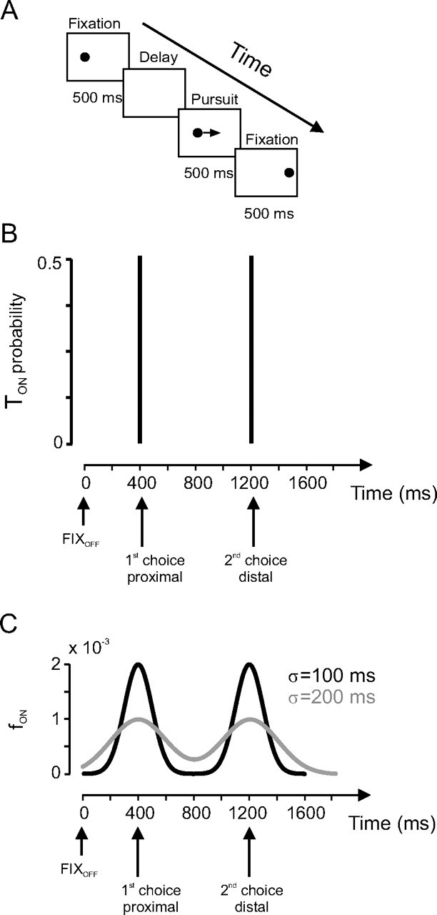
Experimental protocol. A, Sequence of events during a trial. An initial fixation period was followed by a delay period without a stimulus on the screen. At the end of the delay, a target moving at 65°/s appeared at an eccentric position. After 500 ms of target motion, the target stopped for a final fixation period of 500 ms. B, Probability distribution of the time of target motion onset (TON) in the two-choices experiment. Target motion could start either 400 ms after fixation offset (first choice) or 1200 ms after fixation offset (second choice) with the same probability (p = 0.5). C, Bimodal density experiment. Target motion onset TON was drawn from a bimodal density function fON. Black curve, σ = 100 ms; gray curve, σ = 200 ms.
Eye movement measures.
Eye velocity was obtained using a three-point central difference algorithm. We defined anticipatory pursuit as an eye velocity signal >1.5°/s observed between the onset of the fixation period until target motion onset. An additional 100 ms duration criterion was necessary to eliminate trials with an accidental threshold crossing attributable to a transiently increased noise level. We analyzed the influence of the duration and velocity criteria on anticipatory pursuit latency determination. With the velocity criterion fixed at 1.5°/s, three different values of the duration criterion were tested (100, 150, and 200 ms). No significant influence of the length of the duration criterion on median latency was found (Kruskal–Wallis ANOVA, p > 0.05). For a fixed value of the duration criterion (100 ms), four different values of the velocity criterion were tested (1, 1.5, 2, and 2.5°/s). As expected, increasing the value of the velocity criterion significantly increased the median of the latency distributions (Kruskal–Wallis ANOVA, p < 0.05). The average anticipatory pursuit latency was longer for higher-velocity criterion values, and the number of movements that were undetected increased. However, the shape and the spread of latency distributions were not altered by increasing or decreasing the value of the velocity criterion.
In this study, latencies were always measured with respect to the beginning of the delay period (time 0). Differences in the probability distributions of measured variables were tested for statistical significance with the Kolmogorov–Smirnov (KS) test.
In 15% of trials, one or several saccades occurred during the delay period. These trials were not considered for further analysis.
Two temporal choices experiment.
In a first experiment, referred to as “two choices” (Fig. 1B), the delay could take only one of two equally likely values, either 400 or 1200 ms randomly. Trials in which target motion onset (TON) occurred after 400 ms will be referred to as short delay trials. Trials in which target motion onset occurred after 1200 ms will be referred to as long delay trials. At the extinction of the fixation point (FIXOFF), subjects did not know beforehand whether the delay was going to be short or long. This process effectively gave to subjects a temporally proximal (400 ms) or distal (1200 ms) choice of target motion onset.
Bimodal density experiment.
The “bimodal density” experiment was designed to test the influence of temporal uncertainty on anticipatory pursuit responses. The time that elapsed between the offset of the fixation point (FIXOFF) and the onset of target motion (TON) was a random variable drawn from a bimodal density function:
where Gauss is the Gaussian density (Matlab “normpdf” function; Mathworks, Natick, MA), t is elapsed time during the delay period (from 1 to 1600 ms), and σ is the SD of the Gaussians. Two values of σ were tested independently (σ = 100 ms or σ = 200 ms) (Fig. 1C). Subjects experienced a particular σ value for 5 consecutive days before another value was tested. The bimodal density experiment followed the two-choices experiment.
Results
Two temporal choices
In the two-choices experiment, the duration of the delay could take only one of two equally likely values, either 400 or 1200 ms. Figure 2A shows that when the duration of the delay was short, eye velocity typically increased ∼200 ms before expected target motion onset and continued to increase until the onset of visually initiated pursuit. This behavior will be referred to as a single anticipatory response, composed of only one (first) anticipatory movement. When the duration of the delay was long, because target motion did not occur at the time of the first choice, then it would necessarily occur at the time of the second choice (1200 ms with respect to fixation offset). The conditional probability of target motion onset changed as time elapsed past the short delay duration. The behavioral consequences of this change in conditional probability are shown in Figure 2, B and C. Figure 2B shows an example of anticipatory pursuit in the long delay condition when only a single increase in eye velocity was observed during the delay period. The subject anticipated target motion onset after 400 ms, but it did not occur at that time, and a period of fixation followed the anticipatory response. Afterward, the subject waited until target appearance and initiated a visual pursuit movement. This type of behavior will also be referred to as a single response with only one (first) anticipatory movement. Figure 2C shows an example of an anticipatory response with an early and a late increase in eye velocity. Eye velocity increased before the timing of the first choice of target motion onset (400 ms) (Fig. 2C, upward arrow), but afterward, eye velocity started to decrease because no moving target had appeared on the screen. Given that the target had not appeared 400 ms after target motion onset, it became certain that target motion would start 800 ms later. This was reflected in the anticipatory behavior of the subject by a second increase in eye velocity starting ∼300 ms before the second choice of target timing. The second increase in eye velocity continued until the onset of visual pursuit. This type of behavior will be referred to as a double response, with a first and a second movement. The percentage of single and double responses is given in Table 1. During long delays, double responses were more frequent than single responses. Only double responses will be studied here. Indeed, double responses are evidence in favor of the hypothesis that monkeys used an estimate of elapsed time during the delay period combined with an estimation of the probability of TON to decide when to initiate an anticipatory response. The outcome of this decision process is movement initiation, the velocity and latency of which were measured. Figure 3 shows the average velocity of the eye during double responses (A, monkey P; C, monkey T) in the two-choices experiment. In both monkeys, eye velocity increased before the time of the first choice, decreased during the interchoice period, and increased again in expectation of the second timing choice. Corresponding latency distributions are shown in Figure 3B (monkey P) and in Figure 3D (monkey T). In each latency plot, the abscissa represents the time that elapsed from the extinction of the fixation point (time 0) to movement initiation. The ordinate is the corresponding probability of movement initiation. During double responses, two latency distributions could be estimated, for first movements (filled symbols) and for second movements (open symbols). Two important characteristics should be noted. First, the width of the latency distributions for first movements was narrower than the width of the distribution for second movements. This decrease in temporal precision associated with anticipation of the second choice could reflect the influence of the larger temporal delay that has to be estimated between the offset of the fixation point and the time of the second choice of target motion onset. However, the coefficient of variation (CV = σ/μ) computed with the mean and SD of the latency distributions for first and second movements was approximately constant and ∼0.2 (Table 2). Constancy of the CV shows that the variability of movement latencies scales up with the mean latency. Second, the peak of the latency distribution of second movements largely preceded the timing of the second choice, as expected from an anticipatory response to an upcoming certain event.
Figure 2.
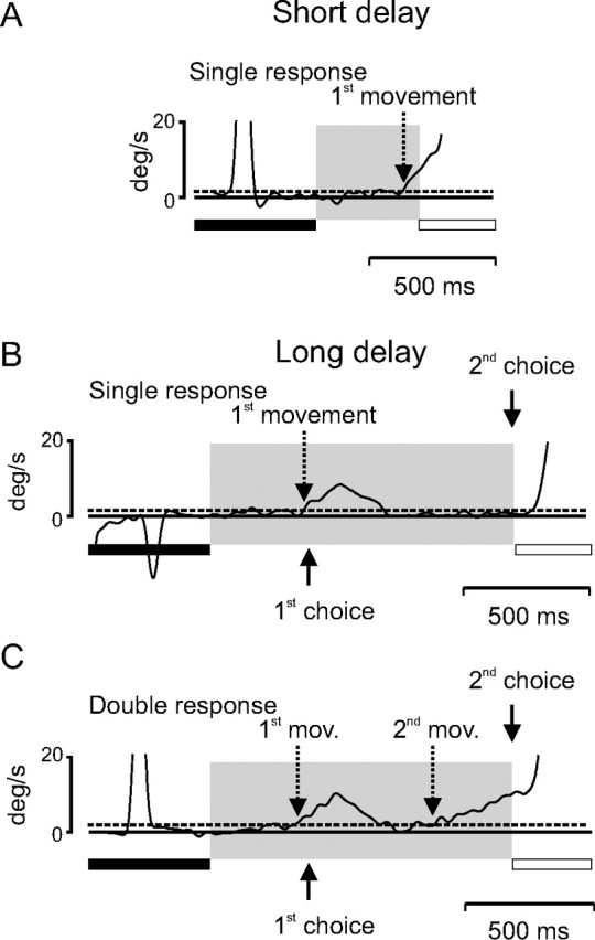
Examples of the different types of anticipatory pursuit movements observed in the two-choices experiment. A, Short delay, single response. Eye velocity is represented as a function of time. The duration of the fixation period is represented with a filled bar below the eye velocity trace. The delay period is represented by a gray area. The target motion period is represented with an open bar. Eye velocity crossed the threshold (dashed line; velocity, 1.5°/s) at the time indicated with a dashed downward arrow. B, Long delay, single response. Eye velocity increased at the time of the first choice (solid upward arrow) and then decreased. Only a single anticipatory pursuit response occurred. C, Long delay, double response. Eye velocity increased before the time of the first choice (solid upward arrow), then decreased and increased again before the time of the second choice (solid downward arrow). Two latencies were measured (1st mov., first movement; 2nd mov., second movement), because eye velocity decreased below the detection level during the intermovement period.
Table 1.
Percentage of single and double responses (two-choices and bimodal density experiments pooled together)
| Monkey | Delay type | Single responses/total responses | Double responses/total responses | Anticipatory trials/total trials |
|---|---|---|---|---|
| Long delays | ||||
| P | (n = 2694) | 308/2694 (11%) | 1515/2694 (56%) | |
| Short delays | ||||
| (n = 2291) | 1457/2291 (64%) | 3280/4985 (66%) | ||
| Long delays | ||||
| T | (n = 1762) | 485/1762 (28%) | 917/1762 (52%) | |
| Short delays | ||||
| (n = 1878) | 884/1878 (47%) | 2286/3640 (63%) | ||
Figure 3.

Two-choices experiment. A, C, Average eye velocity and SD as a function of time for double responses during long delays. B, D, Latency distributions of double responses composed of a first and a second movement. Filled symbols, Latency distribution of first movements; open symbols, latency distribution of second movements; solid lines, Hermite interpolation curves. Data for monkey P are in A and B; data for monkey T are in C and D.
Table 2.
CV of the latency distributions in the two-choices and bimodal density experiments
| Monkey | Two choices |
Bimodal (σ = 100 ms) |
Bimodal (σ = 200 ms) |
|||
|---|---|---|---|---|---|---|
| 1st mov | 2nd mov | 1st mov | 2nd mov | 1st mov | 2nd mov | |
| P | 0.18 | 0.18 | 0.23 | 0.22 | 0.23 | 0.25 |
| T | 0.17 | 0.20 | 0.18 | 0.21 | 0.25 | 0.29 |
1st mov, First movement; 2nd mov, second movement.
Constancy of the CV in double responses suggests a particular instantiation of the scalar variability property for anticipatory pursuit movements (Gibbon, 1977). However, the increased width of the latency distribution of second movements could be explained by two different hypotheses: either it could be attributable to a more error-prone estimation of the timing of the second choice, in agreement with the scalar expectancy theory, or it could be caused by the presence of a preceding first choice that interacts with the planning of the second movements. A control experiment was conducted with three different single choices of delay: 400, 800, and 1200 ms. If the scalar expectancy hypothesis were true, then the width of the anticipatory pursuit latency distribution should increase with the increasing duration of the delay. If the interaction hypothesis were true, then the latency distribution should be unaffected by delay duration. Figure 4A shows the normalized latency distributions for the three delay values tested. Figure 4B shows that the SD of the latency distributions increased with their mean, as predicted by the scalar expectancy theory. As a result, the CV (CV = σ/μ) was approximately constant and ∼10% (0.14, 0.12, 0.09).
Figure 4.

Scalar variability. Three single choices (400, 800, and 1200 ms) were tested independently (indicated with bold and italic characters). A, Distributions of anticipatory pursuit latency when the single choice of target motion onset was either 400 ms (filled squares, continuous line), 800 ms (open circles, continuous line), or 1200 ms (filled circles, dotted line). B, Relationship between mean latency (open circles, dotted line) and SD (Std dev.; filled squares, continuous line) for the three choices tested independently. The mean and the SD covary, and the CV (open squares, continuous line) is approximately constant.
In conclusion, eye velocity changed with the probability of target motion onset during the delay period. Moreover, the estimation of the timing of a distal event (second choice) is more error prone than the estimation of the timing of a proximal event (first choice), but the CV was constant.
Bimodal density
Figure 5, A (monkey P) and B (monkey T), shows the average velocity of the eye during double responses as a function of time during the delay period for the two subjects and the two timing uncertainties tested (black curves, σ = 100 ms; gray curves, σ = 200 ms). In both subjects, when σ = 100 ms, eye velocity increased before the first choice of timing, decreased during the interchoice period, and increased again before the time of the second choice. Two maxima of eye velocity can be observed: the first one around the timing of the first choice and the second one around the timing of the second choice. When σ = 200 ms, eye velocity reached a lower level at the time of the first choice, was maintained at a higher level during the interchoice period, and increased in expectation of the second choice but reached a lower level than for σ = 100 ms.
Figure 5.
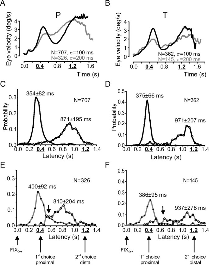
Bimodal density experiment. A, B, Average eye velocity as a function of time for responses when σ = 100 ms (black curves) or σ = 200 ms (gray curves). C–F, Distributions of anticipatory pursuit latency in the bimodal density experiment. Black curves, σ = 100 ms (C, D); gray curves, σ = 200 ms (E, F); filled symbols, first movements; open symbols, second movements. Data for monkey P are in A, C, and E; data for monkey T are in B, D, and F.
The latency distributions of anticipatory pursuit movements were also primarily modified by increasing temporal uncertainty. Figure 5 shows the distributions of anticipatory pursuit latency for all double responses in monkey P (C, E) and monkey T (D, F). The latency distributions of double responses changed with temporal uncertainty. First, peaks of the latency distributions for first and second movements were lower when uncertainty increased (Fig. 5, compare D, F). Second, the width (SD) of distributions increased with temporal uncertainty. The differences between latency distributions for the two σ values tested were all statistically significant (KS test, p < 0.001). Third, the overlap of the latency distributions of first and second movements increased with timing uncertainty. This is manifested by the increasing number of observations in the interval between 0.4 and 0.8 s in the latency distributions (Fig. 5E,F, arrow).
It is necessary to determine which variable, latency or velocity, is primarily altered by timing uncertainty and should be considered for further analysis. To analyze the influence of timing uncertainty on eye velocity, three different variables were measured: the maximum velocity of first and second movements; the velocity of the eye at the time of the first (400 ms) and second (1200 ms) choices; and eye velocity 100 ms after visually guided pursuit onset. Maximum eye velocity during first movements significantly differed in both monkeys (KS test, p < 0.01). For second movements, maximum velocity was not significantly different when uncertainty increased in monkey P (KS test, p = 0.746). In monkey T, the maximum velocity of the eye during second movements was, on average, lower when σ = 100 ms than when σ = 200 ms (KS test, p = 0.001). Eye velocity measured at the time of the first choice was also significantly larger when σ = 100 ms in both monkeys. Eye velocity at the time of the second choice was significantly larger when σ = 100 ms in monkey T (KS test, p < 0.001) but not in monkey P (KS test, p > 0.1). This analysis did not show a clear and systematic influence of timing uncertainty on the velocity of second movements, although latency was significantly altered when uncertainty increased. To determine whether timing uncertainty could alter the transformation of retinal motion signals into a smooth-pursuit command, eye velocity during visual pursuit initiation was also measured. Visual pursuit eye velocity 100 ms after movement onset was not altered by timing uncertainty in monkey P (σ = 100 ms: 53 ± 0.3°/s, n = 632; σ = 200 ms: 53 ± 0.5°/s, n = 292; KS test, p > 0.1) but was significantly altered in monkey T (σ = 100 ms: 37 ± 0.5°/s, n = 340; σ = 200 ms: 33 ± 0.8°/s, n = 138; KS test, p < 0.001). The influence of timing uncertainty on visually guided pursuit velocity differed in both subjects.
In conclusion, the influence of timing uncertainty on anticipatory eye velocity was more variable than its influence on latency. Therefore, in the rest of this study, anticipatory pursuit latency was used as an indicator of the outcome of the temporal estimation process on which the decision to initiate an anticipatory response was made.
Hazard rate
The results presented above could be interpreted by suggesting that monkeys used a perception of elapsed time combined with an estimation of the probability of target motion onset to decide when to initiate an anticipatory movement. This combination can be represented by the hazard rate function.
Mathematically, the hazard rate is defined as follows:
where f(t) is the density function and F(t) is the corresponding cumulative distribution function. The hazard rate is defined for F(t) < 1. We tested whether the hazard functions computed with the fON densities (see Materials and Methods) could appropriately model the outcome of the decision process leading to the initiation of anticipatory pursuit. The hazard functions obtained from the fON densities will be referred to as the “fON hazard rates.” It has been suggested that hazard rates are estimated and used to guide behavior (Ghose and Maunsell, 2002; Janssen and Shadlen, 2005; Oswal et al., 2007). The latency of anticipatory pursuit movements could be considered as the outcome of this process. Therefore, latency hazard rates could be computed from the latency of anticipatory movements. To achieve this, discrete latency distributions were fitted using a shape-preserving interpolation (piecewise cubic Hermite interpolation, Matlab “pchip” function) to generate continuous functions (referred to as the latency densities). Afterward, Equation 2 was applied, and the latency hazard rates were obtained.
Figure 6 shows the comparison of the fON hazard rates (black dashed curves) with the latency hazard rates (gray curves; A,C, σ = 100 ms; B,D, σ = 200 ms; the model hazard rate is the result of a theoretical computation that will be explained below). As shown in Figure 6, A and C, for σ = 100 ms, the fON hazard rates first increased before the time of the first choice, decreased during the interchoices period, and abruptly increased again before the timing of the second choice. Latency hazard rates presented the same increases before the time of the two successive choices, but often ahead of time (note the “shift” between the latency and objective hazard rates) (Fig. 6, compare the A, gray curves, and C, dashed curves). Increases of the latency hazard rates occurred before increases of the fON hazard rates. The advance of the latency hazard rate on the fON hazard rate was relatively larger before the second choice than before the first choice. If subjects tried to match the fON hazard rates, like in a duration reproduction experiment (see Discussion), then the latency hazard rates should at least approximately have the same time course as fON hazard rates. This was not observed. Subjects anticipated the fON hazard rates. This will be quantified with a theoretical model.
Figure 6.

Hazard rates. A comparison of the latency hazard rate functions (gray curves) for σ = 100 ms (A, C) and σ = 200 ms (B, D) with the fON (dashed curves) and model hazard rates (black curves) is shown. Data for monkey P are in A and B; data for monkey T are in C and D.
A theoretical estimation of the latency hazard rate
A simple model was built to estimate the latency densities from the fON densities. The model takes as input a time vector and the mean time of the first and second choice of TON as parameters (μ1 = 400 ms; μ2 = 1200 ms). It provides as output [referred to as the “model densities” (Mod)] an approximation of the latency densities of anticipatory movements according to the following equation:
 |
where Gauss is the Gaussian distribution; t is the time in milliseconds; k is the anticipatory factor (see below); μ1 is the mean time of the first choice, 400 ms; μ2 is the mean time of the second choice, 1200 ms; and si is the SDs.
In this model, two parameters must apparently be determined: the SD of the Gaussians si and the anticipatory factor k. However, as a consequence of the scalar variability property (Fig. 4), the SD of the Gaussians should simply be the product of the mean time of the first or second choice and the CV. Indeed, by definition, CV = s/μ → s = CV × μ. The CVs used to implement the model was 0.2 for σ = 100 ms and 0.3 for σ = 200 ms (Table 2). Therefore, s1 = 80 ms (0.2 × 400 ms) and s2 = 240 ms (0.2 × 1200 ms) for σ = 100 ms. Figure 7A shows the result of applying the scalar variability property to the fON densities (black curve; σ = 100 ms). The result is a probability density with a first peak that is higher and a second peak that is lower than the fON density (Fig. 7A, blue curve).
Figure 7.
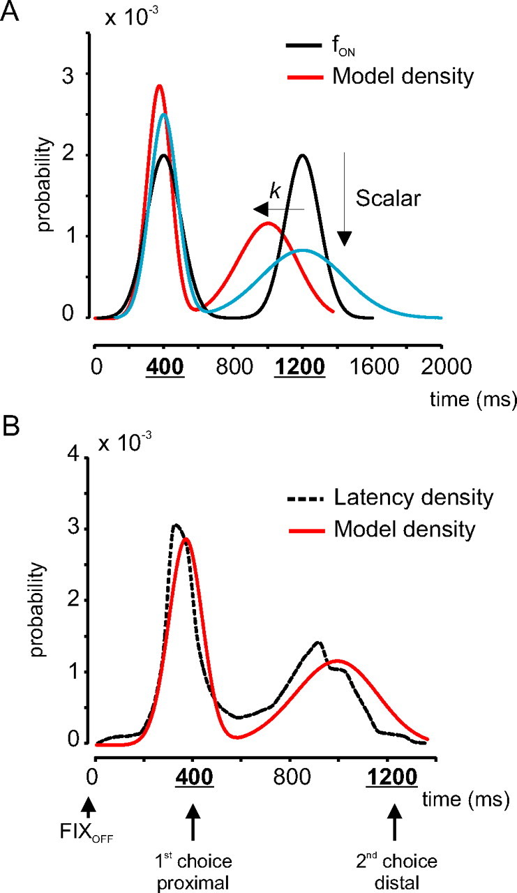
Model predictions and validation. A, Transformation of the fON density (black curve; σ = 100 ms) into the model density (red curve). The blue curve shows the results of the application of the scalar property alone to the fON density (Scalar; downward arrow). B, The dashed curve indicates the latency density for σ = 100 ms in monkey P. The red curve indicates the model density.
Results show that most first movements were, on average, initiated a maximum of ∼50 ms ahead of the time of the first choice. However, second movements started, on average, up to ∼400 ms before the time of the second choice. This was modeled by the anticipatory factor k. We hypothesized that k varied as a function of elapsed time during the delay period preceding TON according to the following equation:
where dt = 1 × 10⁻³, CV = 0.2 (σ = 100 ms) or 0.3 (σ = 200 ms), and k0 = 1.
For each value of time t (by steps of 1 ms), a value of k was computed with Equation 4:
 |
The influence of factor k is weak near the time of the first choice. However, as time elapses during the delay period, the influence of k rapidly increases. As a result, the density for second movements is shifted toward earlier times, as indicated in Figure 7A by a horizontal arrow labeled “k.” Figure 7B shows the comparison between a latency density (black dashed curve; monkey P, σ = 100 ms) and the output of the model (red solid curve). Table 3 shows the values of the variance accounted for by the model and the fON densities. The model was obviously a better predictor of the latency densities than the fON densities. Once the model densities were obtained, the model hazard rates were computed (referred to as “model”) (Fig. 6, solid black curves). Model hazard rates were in good agreement with latency hazard rates for the two temporal uncertainty conditions tested in the two monkeys.
Table 3.
Proportion of the variance of the latency densities accounted for by the fON density or the output of the model (Model): bimodal density experiment
| Monkey | σ = 100 ms |
σ = 200 ms |
||
|---|---|---|---|---|
| fON | Model | fON | Model | |
| P | 0.16 | 0.83 | 0.002 | 0.50 |
| T | 0.46 | 0.87 | 0.34 | 0.58 |
Discussion
We searched for a general mechanism that could describe how anticipatory smooth eye movements are planned in the few hundred milliseconds time range, when both temporal position and uncertainty were varied. This study clearly shows that monkeys relied on a sense of elapsed time and an estimation of prior probabilities to estimate the hazard rate of target motion onset and to decide when to initiate an anticipatory pursuit response.
Increasing timing uncertainty had an influence on both eye velocity and movement latency of double responses. Three different hypotheses could be suggested to explain these results. First, timing uncertainty could primarily affect eye velocity, because the internal gain of the smooth-pursuit pathway was reduced when timing uncertainty increased. The hypothesis has been formulated that the internal gain or “strength” of the transformation of visual signals into smooth-pursuit commands is variable and adjustable. A brief target motion perturbation (a single cycle of a high-frequency sine wave) presented during a fixation period will evoke only a modest smooth eye movement. However, the same perturbation will induce a larger eye velocity response if injected during smooth pursuit (Schwartz and Lisberger, 1994; Churchland and Lisberger, 2002). This internal gain modulation depends of the context of the task (Keating and Pierre, 1996; Krauzlis and Miles, 1996; Tanaka and Lisberger, 2000) and the behavioral conditions (Churchland and Lisberger, 2002). It has been shown recently that the internal gain of smooth pursuit could be altered anticipatively before target motion onset, depending on the probability of target motion (Tabata et al., 2005). Therefore, the lower eye velocity observed when timing uncertainty was increased could also be attributed to a preparatory gain reduction. This will be referred to as the “preparatory gain reduction” hypothesis. Second, movement initiation alone could be primarily affected by increasing timing uncertainty, independently of eye velocity. This will be referred to as the “initiation” hypothesis. Third, a combination of the two precedent hypotheses could be considered. We found that the influence of increasing timing uncertainty was statistically more robust on anticipatory pursuit latency than anticipatory eye velocity, and results were more consistent in the two experimental subjects when latency was used as a dependent variable. Moreover, eye velocity during visual pursuit initiation was not significantly altered by timing uncertainty in one subject. Therefore, the preparatory gain reduction hypothesis does not explain all observed results. The initiation hypothesis suggests that the timing of the anticipatory eye movement initiation could be altered independently of eye velocity. To guide anticipatory responses, subject must rely on a stored representation of target motion or eye movement characteristics. It has been shown that anticipatory pursuit movements are built on a pursuit drive signal (or velocity error) stored in a short-term memory, the content of which is released before the next moving target appears (Wells and Barnes, 1998). The stored information used to drive anticipatory responses can be released by timing cues unrelated to the motion of the stimulus itself (Barnes and Donelan, 1999). Therefore, the storage of the timing of movement initiation and the storage of its velocity could be segregated, perhaps in different neural structures (Barnes and Donelan, 1999). This hypothesis is supported by the results of this study. However, first movements might be more influenced by an anticipatory gain modulation that could occur already during the fixation period, whereas second movements could be initiated on the basis of a perception of elapsed time during the delay period. Therefore, a combination of the initiation and preparatory gain modulation hypotheses might ultimately be the best interpretation.
A theoretical model
To explain the influence of timing uncertainty on movement latency, a simple analytical model was proposed that takes as input the density of target motion onset timing and outputs a latency density. This model is based on the scalar variability property that was found in the present data and on an anticipatory factor k that depended on the CV.
The scalar variability property has been regularly observed in duration reproduction experiments, where subjects have to keep the duration of a reference time interval in working memory and then have to reproduce it. In these conditions, subjects' estimates typically follow a Gaussian distribution centered on the duration of the interval being timed. However, the width of the distribution of estimates increases proportionally with the duration of the interval being timed. Consequently, the CV (σ/μ) is constant. This covariation is referred to as the scalar property of time estimation (Gibbon, 1977; Gibbon et al., 1984; Gibbon and Church, 1990; Church, 2003). The scalar property has been well established in the seconds-to-minutes-to-hours range of timing or interval timing (Rakitin et al., 1998; Kacelnik, 2002; Buhusi and Meck, 2005; Meck, 2005). In this study, we have shown that the SD of the anticipatory pursuit latency distribution increased with the mean of movement latency. Therefore, the present study suggests a particular instantiation of the scalar property in the range of timing characteristic of anticipatory pursuit responses (<2 s).
In the model, the anticipatory factor k depends on the CV value (CV × t2; see Eq. 4) and the value of the measured CV increased with timing uncertainty. This nonlinear factor plays an increasing role as time elapses during the delay period. Indeed, the influence of the CV is proportional to the time squared, and this factor plays a role that is more important for large values of t. This nonlinear factor is causing the early onset of anticipatory responses in expectation of the second choice and the “compression” of the densities toward earlier times. Consequently, the overlap of the first and second movement latency densities increases with uncertainty.
The CV could be considered as representing the sensitivity of the timing process and could be interpreted as a Weber fraction (Weber, 1834) for time estimation (Treisman, 1963a, b; Gibbon, 1977). The increased value of the CV when timing uncertainty increased could be interpreted as if the sensitivity of time estimation was reduced by increasing uncertainty. The confidence of subjects in their timing estimation could consequently be decreased with increasing uncertainty (temporal “blurring”), resulting in an increased SD of the latency distribution and the progressive merging of the latency distributions of first and second movements. This interpretation suggests that increasing timing uncertainty has essentially a disruptive influence, particularly on second movements. However, an alternative interpretation would be to suggest that the increase in SD when σ increased was actually an adaptive learned response. Indeed, even in a changing environment, objects move in a statistically predictable way. Several lines of evidence suggest that the visual system uses the probabilistic structure of the world to efficiently encode information (Knill and Richards, 1996). The pursuit system could estimate and adapt to the increased timing uncertainty of the upcoming event by adjusting the timing of the initiation of the anticipatory response. At this point, the temporal blurring and the adaptive strategy hypotheses form two valid nonexclusive interpretations of the results. Indeed, subjects could try to match the increased dispersion of target motion onset times but only partially succeed in this task. An attempted probability matching would be counteracted by the influence of scalar variability.
Footnotes
This work was supported by the Fonds National de la Recherche Scientifique; the Fondation pour la Recherche Scientifique Médicale; the Belgian Program on Interuniversity Attraction Poles, initiated by the Belgian Federal Science Policy Office; and a Fonds Spéciaux de Recherche internal research grant of the Université Catholique de Louvain. The scientific responsibility rests with its authors.
References
- Badler JB, Heinen SJ. Anticipatory movement timing using prediction and external cues. J Neurosci. 2006;26:4519–4525. doi: 10.1523/JNEUROSCI.3739-05.2006. [DOI] [PMC free article] [PubMed] [Google Scholar]
- Barlow RE, Marshall AW, Proschan F. Properties of probability distributions with monotone hazard rate. Ann Math Stat. 1966;37:1574–1592. [Google Scholar]
- Barnes GR, Asselman PT. The mechanism of prediction in human smooth pursuit eye movements. J Physiol (Lond) 1991;439:439–461. doi: 10.1113/jphysiol.1991.sp018675. [DOI] [PMC free article] [PubMed] [Google Scholar]
- Barnes GR, Donelan SF. The remembered pursuit task: evidence for segregation of timing and velocity storage in predictive oculomotor control. Exp Brain Res. 1999;129:57–67. doi: 10.1007/s002210050936. [DOI] [PubMed] [Google Scholar]
- Blohm G, Missal M, Lefèvre P. Smooth anticipatory eye movements alter the memorized position of flashed targets. J Vis. 2003;3:761–770. doi: 10.1167/3.11.10. [DOI] [PubMed] [Google Scholar]
- Buhusi CV, Meck WH. What makes us tick? Functional and neural mechanisms of interval timing. Nat Rev Neurosci. 2005;6:755–765. doi: 10.1038/nrn1764. [DOI] [PubMed] [Google Scholar]
- Church RM. A concise introduction to scalar expectancy theory. In: Meck WH, editor. Functional and neural mechanisms of interval timing. Boca Raton, FL: CRC; 2003. pp. 3–32. [Google Scholar]
- Churchland AK, Lisberger SG. Gain control in human smooth-pursuit eye movements. J Neurophysiol. 2002;87:2936–2945. doi: 10.1152/jn.2002.87.6.2936. [DOI] [PMC free article] [PubMed] [Google Scholar]
- de Hemptinne C, Lefèvre P, Missal M. Influence of cognitive expectation on the initiation of anticipatory and visual pursuit eye movements in the rhesus monkey. J Neurophysiol. 2006;95:3770–3782. doi: 10.1152/jn.00007.2006. [DOI] [PubMed] [Google Scholar]
- Fuchs AF, Robinson DA. A method for measuring horizontal and vertical eye movement chronically in the monkey. J Appl Physiol. 1966;21:1068–1070. doi: 10.1152/jappl.1966.21.3.1068. [DOI] [PubMed] [Google Scholar]
- Ghose GM, Maunsell JHR. Attentional modulation in visual cortex depends on task timing. Nature. 2002;419:616–620. doi: 10.1038/nature01057. [DOI] [PubMed] [Google Scholar]
- Gibbon J. Scalar expectancy theory and Weber's law in animal training. Psychol Rev. 1977;84:279–325. [Google Scholar]
- Gibbon J, Church RM. Representation of time. Cognition. 1990;37:23–54. doi: 10.1016/0010-0277(90)90017-e. [DOI] [PubMed] [Google Scholar]
- Gibbon J, Church R, Meck W. Scalar timing in memory. Timing and time perception. NY Acad Sci. 1984;423:52–77. doi: 10.1111/j.1749-6632.1984.tb23417.x. [DOI] [PubMed] [Google Scholar]
- Grimmet G, Stirzaker D. Probability and random processes. Oxford: Oxford UP; 2005. [Google Scholar]
- Heinen SJ, Badler JB, Ting W. Timing and velocity randomization similarly affect anticipatory pursuit. J Vis. 2005;5:493–503. doi: 10.1167/5.6.1. [DOI] [PubMed] [Google Scholar]
- Janssen P, Shadlen MN. A representation of the hazard rate of elapsed time in macaque area LIP. Nat Neurosci. 2005;8:234–241. doi: 10.1038/nn1386. [DOI] [PubMed] [Google Scholar]
- Judge SJ, Richmond BJ, Chu FC. Implantation of magnetic search coils for measurement of eye position: an improved method. Vision Res. 1980;20:535–538. doi: 10.1016/0042-6989(80)90128-5. [DOI] [PubMed] [Google Scholar]
- Kacelnik A. Timing and foraging: Gibbon's scalar expectancy theory and optimal patch exploitation. Learn Motiv. 2002;33:177–195. [Google Scholar]
- Keating EG, Pierre A. Architecture of a gain controller in the pursuit system. Behav Brain Res. 1996;81:173–181. doi: 10.1016/s0166-4328(96)89078-4. [DOI] [PubMed] [Google Scholar]
- Knill DC, Richards W. Perception as Bayesian inference. Cambridge, UK: Cambridge UP; 1996. [Google Scholar]
- Kowler E. Cognitive expectations, not habits, control anticipatory smooth oculomotor pursuit. Vision Res. 1989;29:1049–1057. doi: 10.1016/0042-6989(89)90052-7. [DOI] [PubMed] [Google Scholar]
- Krauzlis RJ, Miles FA. Transitions between pursuit eye movements and fixation in the monkey: dependence on context. J Neurophysiol. 1996;76:1622–1638. doi: 10.1152/jn.1996.76.3.1622. [DOI] [PubMed] [Google Scholar]
- Luce RD. Oxford Psychology Series No. 8. Oxford: Oxford UP; 1986. Response times. Their role in inferring elementary mental organization. [Google Scholar]
- Meck WH. Neuropsychology of timing and time perception. Brain Cogn. 2005;58:1–8. doi: 10.1016/j.bandc.2004.09.004. [DOI] [PubMed] [Google Scholar]
- Missal M, Heinen SJ. Supplementary eye fields stimulation facilitates anticipatory pursuit. J Neurophysiol. 2004;92:1257–1262. doi: 10.1152/jn.01255.2003. [DOI] [PubMed] [Google Scholar]
- Oswal A, Ogden MC, Carpenter RH. The time-course of stimulus expectation in a saccadic decision task. J Neurophysiol. 2007 doi: 10.1152/jn.01238.2006. in press. [DOI] [PubMed] [Google Scholar]
- Rakitin BC, Gibbon J, Penney TB, Malapani C, Hinton SC, Meck WH. Scalar expectancy theory and peak interval timing in humans. J Exp Psychol Anim Behav Process. 1998;24:15–33. doi: 10.1037//0097-7403.24.1.15. [DOI] [PubMed] [Google Scholar]
- Schwartz JD, Lisberger SG. Initial tracking conditions modulate the gain of visuomotor transmission for smooth pursuit eye movements in monkeys. Vis Neurosci. 1994;11:411–424. doi: 10.1017/s0952523800002352. [DOI] [PubMed] [Google Scholar]
- Tabata H, Miura K, Kawano K. Anticipatory gain modulation in preparation for smooth pursuit eye movements. J Cogn Neurosci. 2005;17:1962–1968. doi: 10.1162/089892905775008643. [DOI] [PubMed] [Google Scholar]
- Tanaka M, Lisberger SG. Context-dependent smooth eye movements evoked by stationary visual stimuli in trained monkeys. J Neurophysiol. 2000;84:1748–1762. doi: 10.1152/jn.2000.84.4.1748. [DOI] [PMC free article] [PubMed] [Google Scholar]
- Treisman M. Temporal discrimination and the indifference interval. Implications for a model of the “internal clock.”. Psychol Monogr. 1963a;77:1–31. doi: 10.1037/h0093864. [DOI] [PubMed] [Google Scholar]
- Treiman M. Laws of sensory magnitude. Nature. 1963b;198:914–915. doi: 10.1038/198914a0. [DOI] [PubMed] [Google Scholar]
- Weber Annotationes anatomicae et physiologicae. Programmata collecta Leipzig. 1834:1834–1851. [Google Scholar]
- Wells SG, Barnes GR. Fast, anticipatory smooth-pursuit eye movements appear to depend on a short-term store. Exp Brain Res. 1998;120:129–133. doi: 10.1007/s002210050385. [DOI] [PubMed] [Google Scholar]