

Abstract
The dorsomedial entorhinal cortex (dMEC) of the rat brain contains a remarkable population of spatially tuned neurons called grid cells (Hafting et al., 2005). Each grid cell fires selectively at multiple spatial locations, which are geometrically arranged to form a hexagonal lattice that tiles the surface of the rat's environment. Here, we show that grid fields can combine with one another to form moiré interference patterns, referred to as “moiré grids,” that replicate the hexagonal lattice over an infinite range of spatial scales. We propose that dMEC grids are actually moiré grids formed by interference between much smaller “theta grids,” which are hypothesized to be the primary source of movement-related theta rhythm in the rat brain. The formation of moiré grids from theta grids obeys two scaling laws, referred to as the length and rotational scaling rules. The length scaling rule appears to account for firing properties of grid cells in layer II of dMEC, whereas the rotational scaling rule can better explain properties of layer III grid cells. Moiré grids built from theta grids can be combined to form yet larger grids and can also be used as basis functions to construct memory representations of spatial locations (place cells) or visual images. Memory representations built from moiré grids are automatically endowed with size invariance by the scaling properties of the moiré grids. We therefore propose that moiré interference between grid fields may constitute an important principle of neural computation underlying the construction of scale-invariant memory representations.
Keywords: hippocampus, place cell, entorhinal cortex, grid cells, theta rhythm, recognition memory
Introduction
Invariant memory representations make it possible to recognize familiar stimuli independently of their size, position, or context. For example, a resized version of a previously encountered visual image (such as a familiar object viewed from a novel distance) can easily be recognized as familiar, despite the fact that the perceived size of the stimulus has changed. Scale-invariant stimulus recognition is not merely a perceptual phenomenon but seems to reflect underlying properties of the memory representations that encode the familiar stimulus (Jolicoeur, 1987; Biederman and Cooper, 1992). In mammals, the medial temporal lobe memory system is critical for storing memories of familiar stimuli (Eichenbaum, 2004; Squire et al., 2004), so structures within the medial temporal lobe, such as the hippocampus and entorhinal cortex, may contain neural substrates for encoding invariant memory representations. Supporting this, neurons in the human hippocampus and entorhinal cortex can respond invariantly to images of specific people and objects (Fried et al., 1997; Kreiman et al., 2000; Quiroga et al., 2005).
The rodent hippocampus contains neurons called place cells, which are thought to encode memories of specific spatial locations, because each place cell fires selectively whenever the rat returns to a familiar location in space (O'Keefe and Dostrovsky, 1971; O'Keefe and Nadel, 1978; Thompson and Best, 1990; Wilson and McNaughton, 1993). Some place cells seem to encode scale-invariant memory representations of familiar locations, because they can rescale their firing fields when the spatial environment is resized (Muller and Kubie, 1987; O'Keefe and Burgess, 1996; Sharp, 1999; Huxter et al., 2003). Hence, as in humans, neurons in the rodent hippocampus demonstrate a capacity for invariant memory coding.
Hippocampal place cells receive input from neurons called grid cells in the dorsomedial entorhinal cortex (dMEC) (Fyhn et al., 2004; Hafting et al., 2005). Here, we present a computational theory proposing that the hexagonal firing fields of dMEC grid cells are moiré interference patterns, or “moiré grids,” formed from smaller “theta grids” which are hypothesized to be a primary source of theta rhythm in the EEG. Simulations show that this theory can account for the dorsoventral topography of grid field sizes in dMEC (Hafting et al., 2005; Sargolini et al., 2006a) and may also explain why grid cells in layers II and III of dMEC exhibit different phase relationships with the theta EEG (Hafting et al., 2006). We show that moiré grids formed by theta grids can serve as scalable basis functions for constructing size-invariant memory representations, and this may explain how hippocampal place cells rescale their firing fields when a familiar spatial environment is resized. We also show that if a visual image is constructed from a basis set of moiré grids, then the image can automatically be represented at many different sizes within the visual field. In conclusion, we hypothesize that moiré interference between grid fields is a fundamental computational principle underlying the construction of size-invariant memory representations by the nervous system and that small grid fields that produce theta oscillations are the elementary building blocks for constructing such representations in the rodent hippocampus.
Materials and Methods
All simulations were performed using the Matlab programming language (MathWorks, Natick, MA). Firing rate maps of simulated grid cells and place cells were represented by a square matrix of pixels, with each pixel representing the firing rate of the simulated cell at a fixed location.
Definitions of grid field parameters.
As a rat navigates through an open-field environment, grid cells in dMEC fire at multiple vertex locations, which form a hexagonal lattice that tiles the surface of the environment (Hafting et al., 2005). Such a hexagonal lattice can be characterized by three parameters (Fig. 1): the distance between adjacent grid vertices (λ), the rotational orientation of the grid (θ), and the spatial phase of the grid (x0, y0). In the rat brain, different grid cells are tuned to different values of these parameters. The firing field of any particular grid cell maintains stable values of these parameters over time within an unchanging spatial environment (Hafting et al., 2005).
Figure 1.

Simulated grid fields. Example of a simulated grid cell firing field generated by the cosine grating model that was used in our simulations. Hot colors correspond to grid vertices at which the firing rate of the cell is high, and cold colors indicate regions of low firing (the firing rate scale is arbitrary). The hexagonal grid pattern can be characterized by three parameters: grid spacing (λ), angular orientation (θ), and spatial phase [c = (x0, y0)].
Cosine grating model of theta grids.
The model presented in this study proposes that grid cells in dMEC are formed by moiré interference between smaller grid fields, referred to as theta grids because they are hypothesized to produce theta oscillations. We simulated theta grids by summing three cosine grating functions oriented 60° apart, which may be regarded as a simple Fourier model of the hexagonal lattice. This cosine grating model of theta grids was used for computational efficiency and is not intended to represent an accurate biological model of how theta grids are generated in the rat brain. The biological network for generating theta grids is likely to incorporate an attractor network for path integration (Fuhs and Touretzky, 2006; McNaughton et al., 2006), as explained in the Results and Discussion sections. To implement the cosine grating model used in our simulations, we use the Cartesian coordinate vector r = (x, y) to denote an arbitrary spatial position (one square pixel) within a simulated firing rate map. The firing rate of a theta grid G at each spatial location r was simulated as a sum of three cosine gratings as follows:
 |
where the spatial phase of the grid (Fig. 1) was given by c = (x0, y0). The three cosine gratings were oriented along three vectors ω1, ω2, and ω3, which were 60° apart from one another, and these gratings were rotated with respect to the grid field orientation parameter θ (Fig. 1) by angles of θ − 30°, θ + 30°, and θ + 90°. The three vectors had equal length |ωi| = ω, and the length of the vectors determined the vertex spacing of the theta grid, λ, according to the relation λω = 4π/31/2. Here, g was a monotonically increasing gain function given by g(x) = exp[a(x − b)] − 1 with a = 0.3 and b = −3/2. The summation of the three cosine functions had a minimum value of −3/2 and a maximum value of 3, so after passing through the gain function, the value of G(r) ranged from 0 to ∼3 (in arbitrary units). The purpose of the gain function was to disallow negative outputs, because neurons cannot have negative firing rates. The exact choice of gain function is unimportant for the moiré scaling effects reported here.
Spatial resolution of simulated rate maps.
Each square pixel in the firing rate maps corresponded to a square region of physical space. Simulations of moiré grids (see Figs. 4, 5) used pixels measuring 0.1625 cm on each side. Simulations of place cells and grid cells (see Figs. 6–9) used pixels measuring 0.65 cm on each side. Experimental firing rate maps of real place cells were plotted using pixels that measured 3.25 cm on each side; these experimental firing rate maps had to be resampled at a higher resolution to match the resolution of simulated grid fields before weighting coefficients for the model could be fitted to experimental data by Equation 16.
Figure 4.
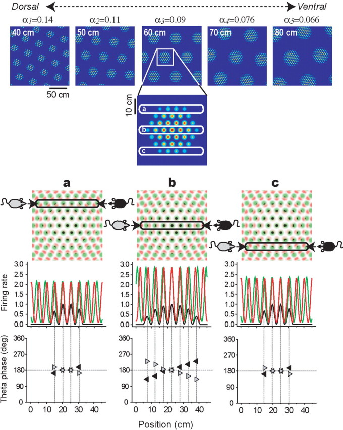
Simulations of layer II grid cells. Top row, Five moiré grid fields, Mi(r), produced by the length scaling rule (Eq. 2); the spacing difference (αi) between theta grids is shown above each plot, and the vertex spacing (Siλ) of each moiré grid is shown at the top left corner of each plot (the hypothetical gradation of αi along the dorsoventral axis of dMEC runs from left to right). Second row, A magnified inset of one moiré grid vertex and three different horizontal cross sections (a, b, and c) through the vertex. Third row, Magnified insets of the theta grids, with Gi(r) plotted in red, Gi((1 + αi)r) plotted in green, and Mi(r) plotted in black. Fourth row, Simulated firing rates (y-axis) of the moiré grid cell (black) and theta grids (red and green) along three horizontal cross sections (columns a, b, and c). Fifth row, The phase of theta rhythm at which Mi(r) peaks on each cycle, with left-to-right traversals shown by gray arrows and right-to-left traversals shown by black arrows; the slopes of these plots show that phase precession occurs as the rat traverses the vertex in either direction (theta EEG is assumed to correspond to the green grid; see Results, Simulating layer II grid cells by the length scaling rule).
Figure 5.
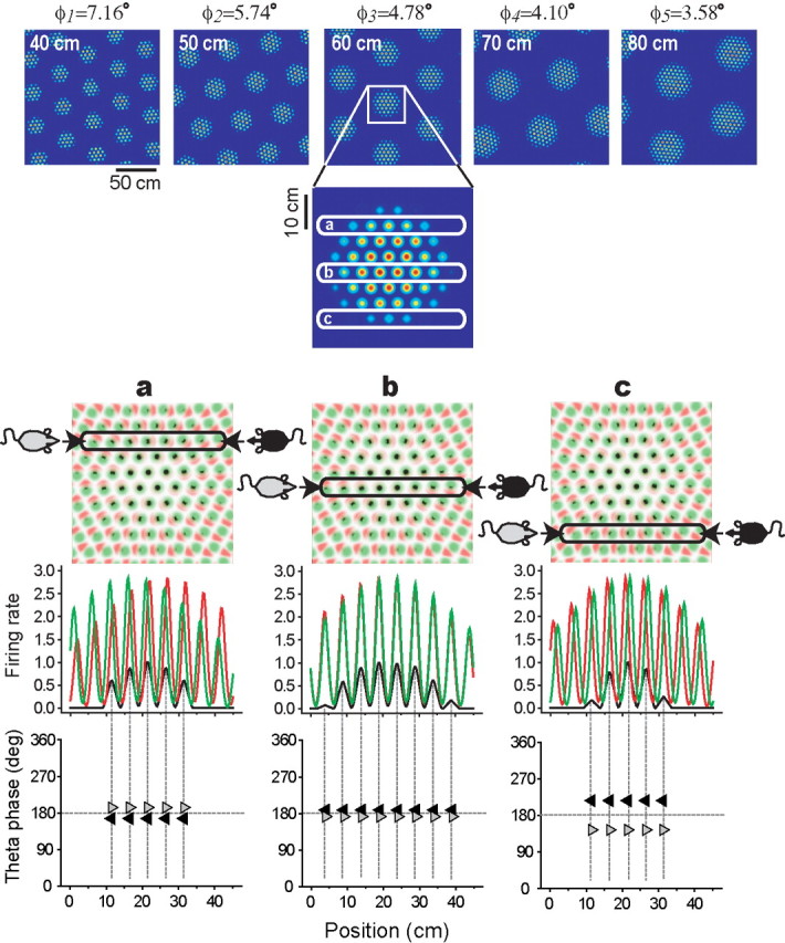
Simulations of layer III grid cells. Top row, Five moiré grid fields, Mi(r), produced by the rotational scaling rule (Eq. 3); the separation angle (φi) between theta grids is shown above each plot, and the vertex spacing (Siλ) of each moiré grid is shown at the top left corner of each plot. Second row, A magnified inset of one moiré grid vertex, with three different horizontal cross sections (a, b, and c) through the vertex. Third row, Magnified insets of the theta grids, with Gi(R(+ϕi)r) plotted in red, Gi(R(−ϕi)r) plotted in green, and Mi(r) plotted in black. Fourth row, Simulated firing rates (y-axis) of the moiré grid cell (black) and theta grids (red and green) along three horizontal cross sections (columns a, b, and c). Fifth row, The phase of theta rhythm at which Mi(r) peaks on each theta cycle for left-to-right traversals (gray arrows) and right-to-left traversals (black arrows). Lateral phase shifting can be seen by comparing across columns a, b, and c. In column b, the rat passes slightly below the center of the vertex, so Mi(r) fires at a slight phase shift from the middle of the theta cycle; in column c, the rat passes farther below the center of the vertex, so Mi(r) fires at a large phase shift from the middle of the theta cycle; in column a, the rat passes above the center of the vertex (farther from the center than in b but not as far as in c), so Mi(r) fires at a moderate phase shift from the middle of the theta cycle (note that in a, the direction of the phase shift is opposite from b and c, because the rat is passing above the vertex center rather than below it). Theta EEG is assumed to correspond to the green grid as in Figure 4.
Figure 6.
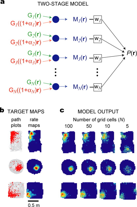
Building place cells from grid cells. a, Diagram of the two-stage model of place cells. b, Path plots (left) and firing rate maps (right) for three real place cells that were recorded in rectangular, circular, and square environments. c, Simulated firing rate maps produced by the two-stage model (see Eq. 15) with different numbers of grid cells in the basis set (N = 100, 50, 10, or 5).
Figure 7.

Place field contractions in the yin–yang maze. The yin–yang maze was contracted from the large (150 cm) to the small (75 cm) configuration during the recording session. a, Firing rate maps are shown for three different place cells recorded before and after maze contraction. b, Simulated firing rate maps constructed from a basis set of 200 grid cells, using different weight vectors (wS and wL) for the small and large rate maps. c, Simulated firing rate maps produced by the moiré model (200 grid cells); coefficients were fit to the large (precontraction) firing rate map (gray background), and the small map was then derived by reducing k from 1.0 to 0.5 without changing the coefficients. d, Overhead view shows how the maze was contracted during the recording session.
Figure 8.

Place field expansions in the yin–yang maze. The yin–yang maze was expanded from the small (75 cm) to the large (150 cm) configuration during the recording session. a, Firing rate maps are shown for three different place cells recorded before and after maze expansion. b, Simulated firing rate maps constructed from a basis set of 200 grid cells, using different weight vectors (wS and wL) for the small and large rate maps. c, Simulated firing rate maps produced by the moiré model (200 grid cells); coefficients were fit to the small (preexpansion) firing rate map (gray background), and the large map was then derived by increasing k from 1.0 to 2.0 without changing the coefficients. d, Overhead view shows how the maze was expanded during the recording session.
Figure 9.
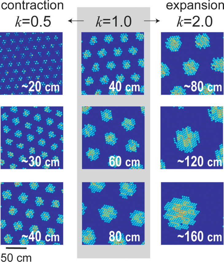
Grid field rescaling. Three moiré grid fields (middle column, gray background) were simulated by the length scaling rule with the scaling parameter set to k = 1 (Eq. 17). When the scaling parameter was reduced to k = 0.5, grids rescaled by approximately halving their vertex spacings (left column). When the scaling parameter was increased to k = 2.0, grids rescaled by approximately doubling their vertex spacings (right column). The vertex spacing of the grid field is shown in the top left corner of each plot; rescaling is approximate rather than exact as explained in Appendix B.
Smoothing of moiré grid fields.
Our theory assumes that theta grids change their vertex spacings as a function of running speed to keep the frequency of theta rhythm constant at all running speeds (see Eqs. 8–10). However, for simplicity, our simulations of place cell rescaling assumed that theta grids have a constant vertex spacing (as if the rat was always running at the same speed) for fixed values of k in Equations 17 and 18. A problem that arises from this simplification is that when a population of moiré grids is resized in unison by adjusting k, the high-frequency components of the moiré grids become shifted in phase relative to one another. The low-frequency components of the moiré grids remain in stable alignment after rescaling, but because the place map is simulated by summing individual pixels in Equation 15, and these pixels have a smaller spatial resolution than the high-frequency components that become realigned, the individual pixels of the moiré grids may no longer sum with one another to produce an output function that has been previously stored by weighting coefficients that were assigned with a different value of k. This problem can be regarded as an artifact of our simplifying assumption that theta grids have constant vertex spacings at all running speeds, because in the case in which theta grids change their vertex spacing as a function of running speed, the vertex spacing (and possibly spatial phase) of theta grids would vary on each traversal of the environment. Hence, moiré grids (and place cells formed from them) would not always fire at the same rate on each traversal through a given spatial location, because the high-frequency component of the grids would be aligned differently on each traversal at different running speeds. This variability would average out over multiple traversals, but it does not average out in our simulations, because we have abolished variability by assuming a constant running speed. To solve this problem, firing rate maps of moiré grid cells, Mi(r), were low-pass filtered by two iterations of smoothing with a square convolution kernel (denoted by K in Equations 11, 13, 17, and 18) measuring 2.0 cm on each side. Smoothing the moiré grids in this way is tantamount to averaging over the variability in the spacing and phase of theta grids that would normally occur over different traversals of the environment at different running speeds.
Experimental place cell recordings.
Target firing rate maps for our simulations were obtained by recording place cells from the CA1 region of the hippocampus in freely foraging rats (provided by A.C.W. and H.T.B.) using methods that have been reported previously (Moita et al., 2004). Briefly, male Long–Evans rats weighing 350–400 g were reduced to 85% of their ad libitum weight through limited daily feeding. Under deep isoflurane anesthesia, microdrives consisting of six tetrode bundles made from 0.0007″ microwire (Kanthal, Palm Coast, FL) were stereotaxically implanted into the dorsal CA1 layer of the hippocampus (coordinates, 3.3 mm posterior, ±3.0 mm lateral, and 1.7 mm ventral to bregma). After recovery, place cells were recorded while rats foraged for food pellets in open-field environments of varying shapes and sizes (see Results). Position data were sampled at 30 Hz by a video tracking system that monitored light-emitting diodes fixed to the rat's head, and single-unit spikes were recorded using multichannel data acquisition and cluster analysis software (Neuralynx, Tucson, AZ). Firing rate maps for each place cell were computed by binning spatial position data into square pixels measuring 3.25 cm on each side. Experimental procedures were approved by the University of California, Los Angeles Animal Care and Use Committee in accordance with federal regulations.
Results
Grid cells in dMEC exhibit vertex spacing lengths that range approximately between 30 and 100 cm (Hafting et al., 2005; Sargolini et al., 2006a), but our model predicts that dMEC grids are built from much smaller grid fields, referred to as theta grids, which we hypothesize to be responsible for producing theta oscillations. Hence, our model posits that at least two different types of grid fields are encoded in the rat brain: dMEC grids and theta grids. Before explaining how these two different grid populations are related to one another, it is necessary to review some general mathematical principles governing moiré interference between hexagonal grid fields.
Moiré interference between grid fields
Suppose that a target neuron receives convergent input from a pair of two different grid cells, each encoding a different grid field. The total input to the target cell would be greatest at spatial locations at which the vertices of the two input grids overlap. Consequently, the target cell would fire in a spatial pattern defined by the regions in which the two input grid fields intersect. It is demonstrated below that the intersection between two hexagonal grids forms a moiré interference pattern, which we shall refer to as a moiré grid, that replicates the hexagonal lattice on a larger spatial scale. Such moiré interference patterns emerge when any two periodic lattices are combined (regardless of their geometry), so the hexagonal lattice is not unique in this regard. But in the present analysis, we shall consider only the case of the hexagonal lattice, because this is the geometric pattern that is generated by grid cells in the rat brain. The size of moiré grid is determined by the parameters of the input grids in accordance with mathematical scaling laws that have been reviewed by Amidror (2000). Here, we present specific formulations of these scaling laws that are specialized for describing hexagonal moiré grids.
The length scaling rule
Consider two hexagonal basis grids that have the same angular orientation but different vertex spacing lengths (Fig. 2). If the vertex spacing length of one basis grid is denoted λ, then the spacing of the other grid can be denoted as λ + αλ, where α is a constant representing the difference in spacing lengths between the two grids (expressed as a percentage of the first grid's spacing length). The intersection of two such grids forms a moiré grid with the same angular orientation as the basis grids but a larger vertex spacing length, Sλ, where S is a scaling factor given by the following:
 |
We refer to Equation 2 as the length scaling rule, because it defines the vertex spacing of the moiré grid as a function of the difference between the vertex lengths of the basis grids. The manner in which moiré grids are produced by the length scaling rule is very similar to the manner in which beat frequencies are produced by interference between sinusoids (Burgess et al., 2005; McNaughton et al., 2006). Just as two sinusoids with slightly different frequencies can sum to produce a lower beat frequency, Equation 2 states that two grid fields with slightly different vertex spacings can sum to produce a larger grid field (a moiré grid). Thus, grid fields can be regarded as two-dimensional (planar) analogues of one-dimensional (linear) sinusoids. As explained below, this kinship between grid fields and sinusoids links our moiré model of grid cells with previous “dual oscillator” models of hippocampal processing (O'Keefe and Recce, 1993; Lengyel et al., 2003; Burgess et al., 2005; O'Keefe and Burgess, 2005).
Figure 2.
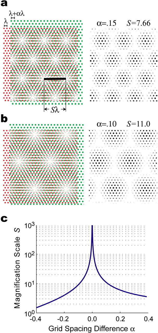
The length scaling rule. a, Two basis grids with identical angular orientation but different vertex spacings, λ (red) and λ + αλ (green), intersect to form a moiré grid shown in black to the right of the basis grids. The vertex spacing of the moiré grid is Sλ, where S is a scaling factor that depends on α. In this example, α = 0.15 and S = 7.66. b, Another example of a moiré grid formed by the length scaling rule, with α = 0.10 and S = 11.0. c, The scaling factor S depends on α, which determines the difference between the spacings of the two basis grids (see Eq. 2).
Moiré interference between grid fields is most robust when there is only a small difference between the vertex spacings of the basis grids (that is, when |α| is near zero); the moiré effect breaks down as |α| grows large (just as sinusoidal beat interference breaks down when the difference between input frequencies is too large). Figure 2c shows that the vertex spacing of the moiré grid can vary over several orders of magnitude as α varies within a small range of values surrounding zero, and S approaches infinity as the vertex spacings of the basis grids approach equivalence (that is, as α vanishes). The spatial phase of the moiré grid is determined by the phases of the two basis grids, but the vertex spacing of the moiré grid is unaffected by the spatial phases of the basis grids.
The rotational scaling rule
The length scaling rule alone does not provide a complete description of moiré interference between planar grid fields, because interference patterns can also be produced by rotating grid fields against one another (an operation which is not possible with sinusoids). When two hexagonal basis grids with identical vertex spacing λ are rotated against one another by an angle φ, they intersect to form a moiré grid with vertex spacing Sλ, where S is a scaling factor given by the following:
 |
We refer to Equation 3 as the rotational scaling rule, because it defines the scale of the moiré grid as a function of the rotation angle between two basis grids with identical vertex spacings. Because this function is periodic at regular intervals of 60°, the moiré pattern formed when the grids are rotated against each other by an arbitrary angle φ is identical to the moiré pattern formed when the grids are rotated against each other by φ + N60° for any integer N. Thus, when analyzing the moiré interference patterns that are formed by rotating two hexagonal grids against one another by an angle φ, it is only necessary to consider angles on the interval 0° ≤ φ < 60°. The angular orientation of the moiré grid formed by rotational scaling is rotated by 30° from the angle that is intermediate between the angles of the two basis grids:
 |
where θ is the orientation of the moiré grid, and θ1 and θ2 are the orientations of the two basis grids that form the moiré grid. The spatial phases of the basis grids are absent from the equations above because the phases of the basis grids do not influence the vertex spacing or orientation of the moiré grid (they affect only the phase of the moiré grid). A relationship similar to the rotational scaling rule was first derived by Lord Rayleigh for parallel line gratings (Stecher, 1964). For the case of hexagonal grids, the rotational scaling principle can be derived by intuitive geometric arguments like those outlined by Oster (1969) or by methods based on Fourier spectra (Amidror, 2000).
Figure 3d shows how the scale S of the moiré grid varies as a function of the rotation angle φ between the basis grids in accordance with the rotational scaling rule. This relation increases monotonically without bound as φ approaches integer multiples of 60°. The smallest value of S occurs when φ = 30° + N60° for integer N, where the scaling function becomes nondifferentiable (for example, see Fig. 3d, the singular point at S = 30°). At these singular points, the moiré magnification factor is equal to S = 1/[2sin(30°/2)] = (2 + 31/2)1/2 ≈ 1.93, an irrational number that we refer to as ζ. Because the scaling factor is irrational when S = ζ, the moiré grid becomes an aperiodic tessellation of the plane that never exactly repeats itself (Fig. 3c).
Figure 3.
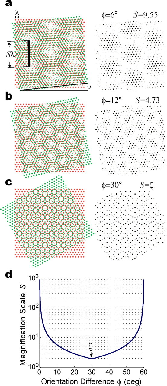
The rotational scaling rule. a, Two basis grids with identical vertex spacing λ and orientations which differ by angle φ intersect to form a moiré grid shown in black to the right of the basis grids. The vertex spacing of the moiré grid is Sλ, where S is a scaling factor that depends on φ. In this example, φ = 6° and S = 9.55. b, Another example of a moiré grid formed by the rotational scaling rule, with φ = 12° and S = 4.73. c, When φ = 30°, the scaling factor becomes irrational (S = ζ), and the moiré grid becomes an aperiodic tessellation of the plane. d, The scaling factor S depends on the separation angle, φ, between the orientations of the basis grids (see Eq. 3); note the irrational singular point at φ = 30°, at which the scale of magnification is S = ζ.
In summary, a pair of basis grids with the same vertex spacing and different angular orientations can be combined using the rotational scaling rule to produce a moiré grid with vertex spacing ranging between λζ and ∞, where λ is the vertex spacing of both basis grids. The spatial phase and orientation of the moiré grid are jointly determined by the phases and orientations of the two basis grids, but the vertex spacing S of the moiré grid is unaffected by the spatial phases of the basis grids, and depends only on the angle of rotation between them.
Generalized moiré scaling law
The length and rotational scaling rules can be combined into a single generalized scaling law that covers all cases in which two basis grids intersect to form a moiré grid, regardless of whether the basis grids differ in their vertex spacing, angular orientation, or both. In general, when two hexagonal basis grids with different vertex spacings, λ and λ + αλ, are rotated against one another by an angle, φ, they intersect to form a moiré grid with vertex spacing Sλ, where S is a scaling factor given by the following:
 |
Variables λ and α in Equation 5 are the same as defined above, and η = min {φ, 60° − φ} to abbreviate the minimum angle term from Equation 3. The angular orientation of the moiré grid is as follows:
 |
where θ1 and θ2 are the orientations of the two basis grids as in Equation 4. Nishijima and Oster (1964) have provided a derivation of this generalized scaling rule for the case of straight-line gratings, and the results for hexagonal grids turn out to be similar. It can be verified algebraically that in the special case when the two grids have identical orientation (that is, φ = θ1 − θ2 = 0), Equation 5 reduces to the length scaling rule of Equation 2. Similarly, in the special case when the two grids have identical spacing (that is, α = 0), Equation 5 reduces to the rotational scaling rule of Equation 3, and Equation 6 is equivalent to Equation 4 (taking into account that θ + N60° represents the same grid orientation for all integer N because of hexalateral symmetry).
Small grid fields produce theta oscillations
The moiré scaling principles outlined above have two important implications for spatial information processing by the grid cell network. First, output from grid cells in dMEC could converge on downstream target neurons to form moiré grids that have much larger vertex spacings than dMEC grid cells (because moiré grids always have larger vertex spacings than the input grids from which they are formed). Second, and perhaps more importantly, dMEC grids might themselves be moiré grids that are formed by summing together much smaller input grids. In this section, we show that small grid fields can produce the movement-related theta oscillations that are known to exist in the hippocampus and entorhinal cortex. We shall hypothesize that these theta grids are the elementary building blocks for constructing spatial memory representations.
Theta grids
Theta rhythm is a 6–8 Hz oscillation that synchronizes neural activity in the hippocampus and entorhinal cortex as a rat navigates through a spatial environment (Vanderwolf, 1969; Mitchell and Ranck, 1980). We hypothesize that this movement-related theta rhythm is produced by small hexagonal grid fields, similar to dMEC grids but with smaller vertex spacing lengths, which we shall refer to as theta grids. To understand how such miniature grid fields could cause theta oscillations during movement, consider a grid field with a small vertex spacing length of λ = 5.0 cm, and suppose that a rat traverses this grid field at a constant running speed of 35 cm/s. If the rat runs along a straight path that is perfectly aligned with a row of grid vertices, then it would pass through 35/5 = 7 grid vertices per second. If a burst of neural activity occurs at each vertex crossing, then the bursts would occur at a frequency of 7 Hz, which is within the frequency range of theta rhythm. More generally, the burst frequency f that would be produced as the rat runs along a row of grid vertices would be as follows:
where V is the running speed of the rat (in cm/s), and λ is the vertex spacing of the grid field (in cm). Equation 7 provides an exact description of the burst frequency only when the rat runs along a straight path that is perfectly aligned with a row of grid vertices. If the rat runs along any other path through the grid, then the burst frequency would be lower than that specified by Equation 7. There are some paths along which vertices might be encountered much less frequently (for example, straight paths rotated exactly 30° from the alignment of the grid field) or even not at all (such as a curved path that avoids grid vertices by weaving in between them), and hence the burst frequency would be much slower than that specified by Equation 7. But a freely behaving rat would be unlikely to travel continuously along such a “vertex-sparse” path for an extended period of time. As long as the diameter of the grid vertices is not too small, most linear (or gently curved) paths through the grid would pass through a vertex at irregularly but similarly spaced intervals, and the mean interval distance would be very close to λ. Thus, Equation 7 provides a good estimate for the frequency of theta bursts that would be produced as a rat runs across a theta grid, even when the rat is not running straight along a row of vertices.
When the rat is standing still, Equation 7 implies that theta rhythm should fall silent, because f = 0/λ = 0. In agreement with this, movement-related theta rhythm in the hippocampus usually falls silent when the rat stops running (Vanderwolf, 1969). However, Equation 7 would predict that the frequency of theta rhythm should be proportional to the rat's running speed with unit slope, so that when the rat runs twice as fast, the theta frequency should also double (because twice as many vertex points would be crossed in the same amount of time). Contradicting this prediction, the frequency of theta rhythm does not double when the rat's running speed doubles; instead, theta rhythm maintains a nearly constant frequency of ∼6–8 Hz across all running speeds. A slight increase in the theta frequency is reported as running speed increases (Whishaw and Vanderwolf, 1973; Rivas et al., 1996; Maurer et al., 2005), but the slope of this increase is much smaller than the unit slope predicted by Equation 7. Thus, experimental data contradicts our hypothesis that theta oscillations are rhythmic bursts produced as the rat traverses through small grid fields. This contradiction may be resolved by postulating that the vertex spacing of theta grids varies systematically with running speed.
Speed-dependent vertex spacing of theta grids
Theta grids can maintain a constant burst frequency by adopting a variable vertex spacing that is directly proportional to the rat's running speed. The vertex spacing of the theta grid must be larger when the rat is running quickly, and smaller when the rat is running slowly, so that the frequency of theta rhythm remains at a constant value. On first consideration, this idea might seem inconsistent with our hypothesis that dMEC grids are moiré grids constructed from theta grids. After all, grid cells in dMEC have stable vertex spacings at all running speeds, so how could they be formed from theta grids with vertex spacings that vary with the rat's running speed?
Consider the case of two theta grids, G1 and G2, which have the same angular orientation but different vertex spacings, so that the vertex spacing of a moiré grid formed by these two theta grids would be determined by the length scaling rule (Eq. 2). Suppose that the vertex spacing of G1 varies with running speed so that the frequency of vertex crossings on G1 (that is, the frequency of theta rhythm) remains constant for all running speeds. We may rearrange Equation 7 to estimate the vertex spacing of G1 as follows:
where λ(V) is the speed-varying vertex spacing of theta grid G1, and f1 is the constant frequency of vertex crossings (theta bursts) produced by G1. Now suppose that the theta grid G1 intersects with another theta grid, G2, to form a moiré grid. For simplicity, we shall assume that G2 always has the same angular orientation as G1, so that the spacing of the moiré grid is given by the length scaling rule (differing orientation is addressed in Appendix A). We shall denote the vertex spacing of G2 as λ(V)[1 + α(V)], where α(V) is the difference between the vertex spacing of G1 and G2, expressed as a percentage of the vertex spacing of G1. This formulation is similar to that used in the length scaling rule above, except that α(V) is now dependent on running speed, a modification that makes it possible to form stable moiré grids from speed-varying theta grids.
The vertex spacing of the moiré grid formed by G1 and G2 is given by Sλ(V), where the scaling factor S is computed from the length scaling rule (Eq. 2). It can be shown algebraically by combining Equations 2 and 8 that Sλ(V) has zero slope (and thus the vertex spacing of the moiré grid is the same for all running speeds) as long as the following is true:
 |
where λM = Sλ(V) is a constant value denoting the fixed vertex spacing of the moiré grid, and f1 denotes the fixed frequency of vertex crossings on G1 (the theta frequency). Hence, a pair of theta grids with speed-dependent vertex spacings can combine to form a moiré grid with a speed-independent vertex spacing, so long as the relative vertex spacings of the theta grids obeys the relation specified in Equation 9. If f1 is a fixed frequency which remains constant at all running speeds, then Equation 9 implies the following:
 |
where f2 is the frequency of vertex crossings on grid G2. Hence, if f1 is constant for all running speeds, then f2 must vary with running speed to form a moiré grid with a stable vertex spacing λM. The approximation in the second step of Equation 10 is quite good, so f2 increases almost linearly with V with a very small slope that is inversely proportional to λM. It is interesting to speculate that Equation 10 might explain why the frequency of theta rhythm is sometimes observed to increase very slightly with the rat's running speed (Whishaw and Vanderwolf, 1973; Rivas et al., 1996; Maurer et al., 2005). If so, then the frequency of theta rhythm recorded in dorsal dMEC (where grid cells have small λM) might be expected to increase more steeply with running speed than theta rhythm recorded in ventral dMEC (where grid cells have larger λM). A biologically plausible mechanism for implementing Equation 9 will be suggested later (see below, A biological mechanism for grid field rescaling). It should be noted that Equation 9 is not the only solution for keeping λM constant at all running speeds while the vertex spacing of theta grids varies. As outlined in Appendix A, other solutions are possible when theta grids differ in their angular orientation instead of their vertex spacing.
Alignment of theta grids with the spatial environment
Hafting et al. (2005) have shown that dMEC grids maintain a stable spatial alignment with familiar visual landmarks. If dMEC grids are moiré grids formed from smaller theta grids, then does this imply that the theta grids must also remain in stable alignment with landmarks? No, not if theta grids change their vertex spacing with running speed to keep the frequency of theta rhythm constant. A moiré grid always has two distinct spatial frequency components: a low-frequency component (the moiré grid itself, which we equate with dMEC grids) and a high-frequency component (the underlying theta grids). The low-frequency component (the moiré grid) can continuously remain in stable alignment with the environment (as dMEC grids appear to do) while the high-frequency theta grids shift their alignment with the environment by dynamically altering their vertex spacing or spatial phase. For example, if the rat's running speed differs on two independent traversals through an environment, then the vertex spacings of theta grids would also be different on each traversal, and theta bursts must therefore occur at different locations with respect to stationary landmarks.
Clearly, the moiré grid must somehow establish and maintain a stable relationship with familiar spatial landmarks, but how can this stability be achieved if theta grids (from which moiré grids are formed) do not maintain a stable alignment with these same landmarks? There are three relationships to consider in answering this question: the alignment of theta grids with landmarks, the alignment of theta grids with moiré grids, and the alignment of moiré grids with landmarks. Importantly, it is possible for each of these three relationships to vary independently of one another. We shall propose later that theta grids are produced by a path integration network (see below, A biological mechanism for grid field rescaling). Prior path integration models have proposed that the integrator can periodically reset its position estimate with respect to visual landmarks, to correct for the accumulation of integration errors over time (Skaggs et al., 1995; Samsonovich and McNaughton, 1997). In a similar way, the theta grid path integrator might periodically reset all three relationships in the moiré network (theta grids to landmarks, theta grids to moiré grids, and moiré grids to landmarks) to correct for the accumulation of integration errors over time. But in between such “reset” events, theta grids could alter their alignment to both the environment and the moiré grids, without upsetting the alignment between the environment and the moiré grids. Therefore, in its current form, our theory does not offer specific predictions about the stability of the alignment between theta grids and the environment over time.
Sensitivity of the moiré scaling mechanism
The slopes of the moiré scaling functions are quite steep (Figs. 2c, 3d), so small fluctuations in the spacing or orientation of theta grids would cause large fluctuations in the size of moiré grids produced by the theta grids. This might be problematic in a biological network, because small levels of input noise could cause large fluctuations in the scale of the spatial representation produced by the network. Clearly, the accuracy of the spatial relationships between theta grids would have to be maintained within very strict tolerances to produce moiré grids with stable vertex spacings, and this is potentially a serious limitation of our model.
Simulations of dMEC grid fields
We shall now present simulations to demonstrate that key firing properties of dMEC grid cells can be accounted for by the hypothesis that dMEC grids are moiré grids formed from smaller theta grids. For simplicity, our simulations shall assume that theta grids have constant vertex spacings (as if the rat is always traveling at a constant running speed), because this makes it easier to visualize the moiré interference principles that we wish to demonstrate. Thus, running speed will not be included as a variable in the model equations. However, it should be understood that the principles of moiré interference that we describe in our simulations are not altered by this simplifying assumption, and in the rat brain, theta grids may have vertex spacings that vary with running speed to keep the theta frequency nearly constant (as specified by Equations 8 and 9 and in Appendix A).
Simulating layer II grid cells by the length scaling rule
Grid cells in layer II of dMEC are topographically organized so that cells in dorsal regions of dMEC have small vertex spacings of ∼30 cm, and the spacing grows progressively larger at more ventral locations, reaching a maximum of ∼100 cm in the most ventral portion of dMEC (Hafting et al., 2005; Sargolini et al., 2006a). Layer II grid cells also exhibit phase precession with respect to the locally recorded theta EEG (Hafting et al., 2006), so that as the rat traverses each grid vertex, the grid cell fires at a late phase of the theta EEG cycle as a rat enters the vertex and at an early phase as the rat leaves the vertex. This is similar to theta phase precession that is observed for place cells in the hippocampus (O'Keefe and Recce, 1993; Skaggs et al., 1996; Maurer et al., 2006).
O'Keefe and Burgess (2005) have hypothesized that both of these properties of grid cells (the dorsoventral topography of their grid spacings and their theta phase precession behavior) can be accounted for by interference between sinusoids of differing frequency. Burgess et al. (2005) extended this idea into two dimensions, showing that these grid cell firing properties can be similarly accounted for by interference between hexagonal grid fields with different vertex spacings. Here, we shall demonstrate a similar result, by showing that these grid cell firing properties are inherent to moiré grids that are formed using the length scaling rule of Equation 2.
To simulate a population of layer II grid cells using the length scaling rule, a set of moiré grids was produced from “sibling pairs” of theta grids. The firing rate of the ith moiré grid cell at spatial location r was given by the following:
where Gi(r) and Gi((1 + αi)r) are the ith pair of sibling theta grids, μM = 4.0 is an activation threshold, []+ denotes thresholding such that the expression inside the brackets is taken to be zero for negative values, * is the convolution operator, and K is a kernel for smoothing the moiré grid field (see Materials and Methods). The ith theta grid cell Gi(r) was simulated by the cosine grating model described in the Materials and Methods section, and its sibling Gi((1 + αi)r) was derived by scaling Gi(r) about the origin of the coordinate axis. Both of the sibling theta grids, Gi(r) and Gi((1 + αi)r), had the same angular orientation θi, so that the orientation of the moiré grid Mi(r) was also equal to θi. In simulations presented here, the vertex spacing of the first theta grid Gi(r) was always λ = 5.0 cm, and the spacing of the second theta grid was given by λ + αiλ (with αi > 0). Thus, the vertex spacing of each Mi(r) was determined solely by its αi parameter.
Figure 4 (top row) shows five examples of simulated moiré grid fields Mi(r) spanning a range of vertex spacings from 40 to 80 cm along the dorsoventral axis of dMEC. To obtain this gradation of grid spacings, the value of the αi parameter was incrementally changed along the interval 0.1429 ≥ αi ≥ 0.0667, which produced moiré grid spacings in the range 40 ≤ Siλ ≤ 80 cm when λ = 5.0 cm (this can be verified from Equation 2). These simulations suggest that the topography of vertex spacings for layer II grid cells may arise because the αi parameter is graded along the dorsoventral axis of dMEC. That is, ventrally located grid cells receive inputs from pairs of theta cells with very similar vertex spacings (αi very near to zero), thereby producing large moiré grid fields. In contrast, grid cells in dorsal layer II receive input from pairs of theta grids with less similar vertex spacings (αi larger but still near zero), thereby producing small moiré grid fields. This explanation is very similar to O'Keefe and Burgess' (2005) hypothesis that the topography of grid spacings in dMEC arises from a dorsoventral gradient of frequency pairings between sinusoidal oscillators, except that here, theta grid vertex spacings are substituted for sinusoidal frequencies.
The moiré grid vertices produced by the length scaling rule have a grainy appearance, which is caused by the high spatial frequency of the underlying theta grids from which the vertices are formed. Figure 4 (second row) shows a magnified view of a single grid vertex, to illustrate how the vertex is produced by moiré interference between the underlying pair of theta grids. Figure 4 (third row) shows a magnified view of the sibling theta grids that form the vertex, with Gi(r) plotted in red and Gi((1 + αi)r) plotted in green; black regions in this plot show the points of overlap between the theta grids, which are locations where the grid cell Mi(r) would fire action potentials. The phase relationship between theta rhythm and the firing of layer II grid cells can be inferred from this plot by assuming that the peaks and troughs of the theta EEG correspond to the peaks and troughs of the theta grid plotted in green, Gi((1 + αi)r). The black spots at which the grid cell fires can be seen to precess backward in phase through one cycle of the theta rhythm on each traversal of a grid vertex in any direction. To better illustrate this, Figure 4 (fourth row) shows horizontal cross sections through the grid vertex at varying distances from the vertex center (a, b, and c). In cross section, the two theta grids become a pair of detuned sinusoids (red and green), and the moiré grid vertex becomes a sequence of small bumps that together form a larger bump (black). The phase precession phenomenon emerges from interference between the sinusoids, exactly as in dual oscillator models of phase precession by place cells while rats are running on a linear track (O'Keefe and Recce, 1993; Lengyel et al., 2003; O'Keefe and Burgess, 2005). Hence, the length scaling rule can properly be regarded as an extension of these dual oscillator models into two dimensions (Burgess et al., 2005).
Figure 4 (bottom row) plots the phase of theta rhythm at which the grid cell fires (y-axis) for each horizontal position along the grid vertex (x-axis). Time progresses either from left to right or right to left along the x-axis, depending on which direction the rat is moving (rightward vs leftward, respectively). The phase plot is negatively sloped with respect to position when the rat travels rightward (gray triangles), and positively sloped when the rat travels leftward (black triangles), so grid cell spiking always precesses backward through the phase of theta rhythm. It can also be seen in the two-dimensional theta grid plot (Fig. 4, row 3) that backward phase precession occurs regardless of the angle at which the cross section is taken through the grid vertex. It must be assumed that the local theta EEG in layer II measures vertex crossings on the larger theta grid (green) and not the smaller one (red), because if the theta EEG were produced by vertex crossings on the smaller theta grid, then grid cell spikes would shift in the wrong direction through the theta phase (forward instead of backward), in conflict with experimental data. To account for this, it may be assumed that all of the grid cells within a local region of layer II receive shared input from a common “master” theta grid, so that their membrane potentials oscillate synchronously to produce a field potential that is observable as theta rhythm in the EEG. In addition to input from the master grid, each grid cell may also receive input from a secondary theta grid with a smaller vertex spacing than the master grid, which would interfere with the master grid to form a moiré grid. Unlike the master grid, which is shared among all grid cells, the secondary theta grid would be different for each dMEC cell. Thus, the secondary grids would not oscillate in synchrony and would not be detectable by EEG. The secondary theta grid signal might arrive through unique synaptic inputs to each grid cell or it might somehow be encoded by intrinsic oscillatory membrane properties that are unique to each grid cell, as in previous implementations of dual oscillator phase precession models (Lengyel et al., 2003).
Simulating layer III grid cells by the rotational scaling rule
Grid cells in layer III of dMEC seem to differ from grid cells in layer II in two major respects. First, the dorsoventral gradation of grid spacings is poorly organized, so that neighboring layer III grid cells can have very different vertex spacings even though they are located at the same dorsoventral coordinate position (Sargolini et al., 2006a). Second, layer III grid cells often do not show theta phase precession during traversal of a grid vertex (Hafting et al., 2006). These firing properties suggest that layer III grid cells are not formed by the length scaling rule. It is demonstrated below that these firing properties layer III grid cells might instead be explained by the rotational scaling rule.
To simulate a population of dMEC grids using the rotational scaling rule, moiré grids were again produced from sibling pairs of theta grids, except that this time, the sibling theta grids differed in their angular orientations rather than their vertex spacings. It was mathematically convenient to obtain each sibling pair of theta grids by rotating a common “parent” theta grid by the same angle ϕi in opposite directions (thus, the orientation of the parent grid was intermediate between the orientations of the siblings). Using this formulation, the orientation θi of the moiré grid always remained constant when the angle between the theta grids was adjusted by changing ϕi. By Equation 4, the orientation of the parent grid must equal θi − 30° to produce a moiré grid with orientation θi. Hence, the orientations of the two siblings were θ − 30° + ϕi and θ − 30° − ϕi, and the rotation angle between the two theta grids that formed the moiré grid was as follows:
Using this method for obtaining theta grids, the firing rate of the ith moiré grid cell at location r was given by the following:
 |
where Gi(R(−ϕi)r) and Gi(R(+ϕi)r) are the ith pair of sibling theta grids, and all other terms are exactly as in Equation 11 above. The siblings Gi(R(−ϕi)r) and Gi(R(+ϕi)r) were derived by rotating a common parent grid Gi(r) by equal angles in opposite directions using the following rotation matrix:
 |
Both theta grids had the same vertex spacing, which was always equal to λ = 5.0 cm. The parent grid Gi(r) was simulated using the cosine grating model (see Materials and Methods), and the orientation of the ith parent grid was defined as θi − 30°, so that the orientation of the ith moiré grid Mi(r) would be equal to θi in accordance with Equation 4.
Figure 5 (top row) shows five examples of simulated moiré grid fields Mi(r) spanning the range of vertex spacings from 40 to 80 cm. To obtain this gradation of grid spacings, the value of the ϕi parameter was incrementally changed along the interval 3.58° ≥ ϕi ≥ 1.79°. It can be verified from the rotational scaling rule (Eq. 3) that this range of separation angles between theta grids produces moiré grid spacings in the range 40 ≤ Siλ ≤ 80 cm when λ = 5.0 cm. Hence, unlike in layer II, in which grid cell spacings were controlled by the αi parameter, the vertex spacing of layer III grid cells was controlled by the ϕi parameter. If the αi parameter is graded along the dorsoventral axis of dMEC, but the ϕi parameter is not, then this could explain why layer II grid spacings are topographically organized along the dorsoventral axis, whereas layer III grid spacings are not as rigidly organized along the dorsoventral axis (Sargolini et al., 2006a).
Figure 5 (second row) shows a magnified view of a single grid vertex, and Figure 5 (third row) shows a magnified view of the sibling theta grids that form the vertex, with Gi(R(−ϕi)r) plotted in red and Gi(R(+ϕi)r) plotted in green; black regions show the points of overlap between the theta grids, which are locations at which the grid cell Mi(r) would fire action potentials. The phase relationship between theta rhythm and the firing of layer III grid cells can be inferred from this plot by assuming that the peaks and troughs of the theta EEG correspond to the peaks and troughs of Gi(R(+ϕi)r), the grid plotted in green. Notice that the black spots, at which the grid cell fires, remain at the same phase within the theta rhythm on each traversal of a grid vertex in any direction (although there is a lateral shift of the black spots, addressed further below). To better illustrate this, Figure 5 (fourth row) shows horizontal cross sections through the grid vertex at varying distances from the vertex center (a, b, and c). In cross section, the two theta grids become a pair of sinusoids with the same frequency (red and green), and the moiré grid vertex becomes a sequence of small bumps that together form a larger bump (black). Figure 5 (bottom row) plots the phase of theta rhythm at which the grid cell fires (y-axis) at each position within the grid vertex (x-axis) as the rat traverses the vertex in either direction. The phase plot is always flat for both left-to-right traversals (gray triangles) and right-to-left traversals (black triangles), showing that the grid cell fires at the same theta phase throughout each traversal in either direction; thus, phase precession does not occur.
Lateral phase shifting: a novel prediction of the model
Although phase precession does not occur for grid cells formed by the rotational scaling rule, the phase at which the grid cell fires does depend on where the rat passes through the vertex. Figure 5 shows that when the rat passes near the center of the vertex (row b), the grid cell fires at a constant phase near the middle of the theta cycle. When the rat passes through the edges of the vertex, the grid cell fires early in the theta cycle at one edge and late in theta cycle at the other edge (rows a and c). Consequently, the grid cell exhibits lateral phase shifting from the left to the right edges of the grid vertex, rather than from the front to the back of the vertex as in classical phase precession.
This lateral phase-shifting effect is a prediction of the model that can be tested by recording grid cells from dMEC in an open-field environment. If some dMEC grid cells are formed by the rotational scaling rule, then these cells should exhibit lateral phase shifting of their spikes with respect to the local theta EEG. Hence, whenever the rat passes through a grid vertex on one side (e.g., the left edge), the grid cell's spikes should occur at a particular phase within the theta cycle (e.g., early). If the rat passes through a vertex of the same grid cell on the opposite side of its center (e.g., the right edge), then the grid cell's spikes will occur at the opposite phase within the theta cycle (e.g., late). If this prediction were to be verified, it would provide very strong evidence that some dMEC grids are indeed formed by the rotational scaling rule and thereby support our hypothesis that theta rhythm is produced by grid fields with small vertex spacings.
Simultaneous forward and lateral phase shifting
Some dMEC grids might be moiré grids which are formed by the generalized scaling rule of Equation 5, so that they are constructed from theta grids that differ both in their orientation and their vertex spacing (rather than just one or the other, as in Figs. 4 and 5). In such cases, grid cells would simultaneously exhibit standard phase precession (as in Fig. 4) as well as lateral phase shifting (as in Fig. 5). Hence, grid cells in dMEC might exhibit both forward and lateral phase shifting at the same time, rather than just one or the other, depending on how they are formed from theta grids.
Building place cells from grid cells
Place cells in the hippocampus receive inputs from grid cells in dMEC (Fyhn et al., 2004), so place cells could form their location-specific firing fields by summing inputs from dMEC grid cells (Fuhs and Touretzky, 2006; McNaughton et al., 2006, Solstad et al., 2006). To simulate location-specific firing in place cells receiving convergent input from a population of moiré grid cells, we used a two-stage feedforward model (Fig. 6a). In the first stage, sibling pairs of theta grids were combined to form moiré grid cells, Mi(r). In the second stage, outputs from Mi(r) were linearly summed to create a place cell firing field according to the following equation:
 |
where r = (x, y) denotes an arbitrary Cartesian position within a simulated firing rate map, P(r) is the output of the model, which corresponds to the mean firing rate of a simulated place cell at location r, Mi(r) is the mean firing rate at location r of the ith moiré grid cell, N is the number of grid cells projecting onto the simulated place cell, and w1, w2, · · ·, wN are the weighting coefficients of synaptic inputs onto the place cell from each grid moiré cell. For place cell simulations presented here, the activation threshold μP was set equal to 25% of the maximum value of ΣiN = 1 wiMi(r) over all locations r.
Input to the feedforward model was provided by a basis set consisting of moiré grid cells, Mi(r). Moiré grid cells can be generated using either the length scaling rule to simulate layer II grid cells (Eq. 11) or the rotational scaling rule to simulate layer III grid cells (Eq. 13). For simplicity, place cell simulations presented here used a basis set of moiré grids formed only by the length scaling rule (Eq. 11). Parameters of the simulated grid cell population Mi(r) were assigned randomly from distributions matching the spatial tuning properties of real grid cells in layer II of dMEC. Thus, grid orientations were distributed uniformly in the range 0° ≤ θ < 60°, and spatial phases of each grid field were uniformly distributed throughout the plane. Vertex spacings of the population Mi(r) were distributed uniformly in the range 30 < Siλ < 80 cm; this was achieved by setting λ = 5.0 cm (as in Fig. 4) and randomly assigning vertex spacing differences from the interval 0.2 ≥ αi ≥ 0.0667. The number of grid cells in the population (N) was varied in different simulations to study how the size of the basis set influenced the fitting accuracy of the model.
The weighting coefficients w1, w2, · · ·, wN were chosen to minimize the mean square error between the output of the model, P(r), and a target function, T(r), which was the firing rate map of a real hippocampal place cell. An approximation of the best fit for the coefficients was obtained by ignoring the nonlinearity in Equation 15 and setting w1, w2, · · ·, wN as follows:
 |
where † denotes Moore–Penrose pseudoinverse, t is a column vector obtained from T(r) by concatenating the firing rate values for all of the spatial pixel bins that were visited by the rat, and [m1, · · ·, mN] is a matrix with each column mi obtained from Mi(r) in the same manner as t. The solution for the optimal weight vector is unique as long as the matrix is full rank, which is typically the case when there are more spatial pixels than the number of grid cells. In this solution, each weight wi can be either positive or negative. In a biologically plausible implementation of the model, inhibitory projections from grid cells onto place cells would be mediated by an intermediate layer of feedforward inhibitory interneurons. However, for simplicity, the implementation used here consists of a single feedforward layer in which synaptic weights can assume both positive and negative values derived directly from Equation 16.
Simulation results
Figure 6b shows examples of path plots and firing rate maps from real CA1 place cells recorded in three different spatial environments: a rectangle, a circle, and a square. The firing rate map of each place cell was used to derive a target vector, t, from which the weighting coefficients of the model were derived using Equation 16. Before fitting, the target firing rate map t of each place cell was resampled at a higher pixel resolution to accurately represent the high spatial frequencies of the theta grids that provided input to the first stage of the model (see Materials and Methods). Figure 6c shows simulated firing rate maps produced by the model using different numbers of basis grids at the input stage: N = 100, 50, 10, or 5 grid cells. When the size of the basis set was small, the model produced only a crude approximation of the firing rate map of the place cell. However, as the size of the basis set increased, simulated firing rate maps became more similar to the target maps.
Scale-invariant place fields
When the boundaries of a familiar spatial environment are expanded or contracted, place cells can sometimes rescale the size and position of their firing fields to match the new dimensions the environment (Muller and Kubie, 1987; O'Keefe and Burgess, 1996; Sharp, 1999; Huxter et al., 2003). This suggests that some place cells may encode the same relative position within a familiar environment, regardless of the size of the environment. That is, some place cells may encode scale-invariant representations of specific locations within a familiar environment.
This rescaling phenomenon is illustrated by place cell recording data shown in Figures 7a and 8a. Place cells were recorded from dorsal CA1 while rats foraged in an apparatus called the yin–yang maze (an adjustable cylinder with flexible walls that could be expanded or contracted to adjust the maze diameter during the recording session without removing the rat from the maze) (Figs. 7d, 8d). Figure 7a shows three place cells that were recorded during contractions of the maze; these cells were recorded while the maze was set to a large diameter (150 cm), and then the maze was contracted to the small diameter (75 cm) without removing the rat, and the same place cells were recorded again in the smaller maze. Figure 8a shows similar data from three place cells that were recorded during expansions of the maze (first in the small maze and then in the large maze). It can be seen from Figures 7a and 8a that when the maze was resized, the size and position of place cell firing fields changed nearly proportionally along with the size of the maze, as in previous studies showing that CA1 place cells can rescale the size of their firing fields when the dimensions of a familiar environment are altered (Muller and Kubie, 1987; O'Keefe and Burgess, 1996; Sharp, 1999; Huxter et al., 2003).
How can place cells rescale their firing fields in response to resizing the dimensions of a familiar environment? One theory has proposed that place cells may receive inputs that encode “boundary vectors” representing distances between the rat and the boundaries of its environment (O'Keefe and Burgess, 1996; Barry et al., 2006). This theory can account for a variety of different place cell responses that are observed when boundaries are inserted, removed, or resized in a familiar environment. However, if place cells derive their location-specific firing properties by summing inputs from grid cells (rather than boundary vectors), then an alternative explanation for place field rescaling may be required. Two such alternative explanations will be considered below.
Place field rescaling by weight refitting
One possibility is that place cells might rescale their firing fields by “refitting” the weighting coefficients of their grid cell inputs. That is, each place cell might change the strengths of its synaptic inputs from grid cells when the environment is resized, thereby producing a rescaled version of its original place field. To investigate whether such weight refitting can account for place field rescaling, firing rate maps from recording sessions in the yin–yang maze were used to generate target vectors, t, for fitting the weight coefficients of our feedforward model (exactly as in the simulations of Fig. 6c above). Because each place cell was recorded twice in the yin–yang maze (once in the large and once in the small maze configuration), there were two different target vectors for each cell: tS (small maze) and tL (large maze). Fitting the model to these two target vectors (using Equation 16) yielded two different sets of weighting coefficients for each place cell: wS = (w1S, w2S, · · ·, wNS) (small maze) and wL = (w1L, w2L, · · ·, wNL) (large maze). Input to the model was provided by a fixed basis set of N = 200 simulated grid cells with randomly chosen parameters as in simulations above.
Figures 7b and 8b show examples of the model's output, which very accurately reproduced the target maps of cells recorded in both the small and large maze configurations, using a separate weight vector (wS and wL) for each size of the maze. These simulations results suggest that in principle, it is possible for place cells to rescale their firing fields by refitting their weighting coefficients when a familiar environment is resized. However, there is a drawback to this weight-refitting model of place field rescaling: it has one free parameter (the weight coefficient) for each grid cell in the basis set. For large basis sets, the number of free parameters in the model could grow dauntingly large, and it is unclear how a place cell could recompute its input weight vector to encode arbitrary changes in the size of an environment over a continuous range. We shall now propose an alternative model of place field rescaling which exploits moiré grid fields. Unlike the weight-refitting method, the moiré scaling model proposed below has only three free parameters no matter how many grid cells there are in the basis set.
Moiré model of place field rescaling
Consider a place field P(r) that is constructed from a basis set of moiré grids Mi(r), as specified by Equation 15. If all of the moiré grids Mi(r) in the basis set are rescaled in unison by a common scaling factor k about a common scaling origin (xS, yS), then P(r) will be rescaled by the same factor k about the same scaling origin (xS, yS). Therefore, a biological mechanism for rescaling the population of moiré grids would automatically provide a biological mechanism for rescaling place fields.
Recall that in the two-stage moiré model of place cells that was presented above (Fig. 6a), the first stage of the model combined pairs of theta grids to produce moiré grids in accordance with the length scaling rule (Eq. 11). Each moiré grid cell Mi(r) was formed by summing input from two theta grids, Gi(r) and Gi((1 + αi)r). The vertex spacing of Gi(r) was fixed at λ = 5.0 cm, and the vertex spacings of Mi(r) were determined by αi. An interesting property of moiré grids constructed in this way is that if all of the αi parameters are divided by the same scaling factor k, then the vertex spacings Siλ of all of the moiré grids Mi(r) become rescaled in unison, approximately by the factor k. This principle can be implemented in our model by a slight modification of Equation 11, in which we substitute αi with αi/k as follows:
After this modification, the vertex spacing of Mi(r) is still given by Siλ, but now Si is obtained by substituting αi/k for αi in the length scaling rule (Eq. 2). When moiré grids are generated using Equation 17, the spatial scale of all Mi(r) can be regulated in unison by a single scaling parameter k.
Rescaling of Mi(r) by k is approximate and not exact, as explained in Appendix B. Figure 9 shows how adjusting the value of k affects the vertex spacings of moiré grids produced by Equation 17. Adjusting k does not alter the orientations or the relative phases of Mi(r), as long as the scaling axis is fixed at the same point for all Mi(r). In Figure 9, the scaling origin is located at the center of each square plot. Hence, adjusting the parameter k can rescale the entire population of moiré grids in unison. If we simulate a place cell P(r) as a sum of weighted inputs (Eq. 15) from scalable moiré grid cells Mi(r) that are generated by Equation 17, then the simulated place field will also rescale along with k. Hence, a place field constructed from a scalable basis set of moiré grids can be rescaled by setting only three free parameters: the scaling factor k and the x and y coordinates of the scaling origin (xS, yS). Unlike the weight-refitting model, the number of free parameters for rescaling does not increase with the size of the basis set.
A two-stage moiré interference model was used to simulate the rescaling of place fields in experiments with the yin–yang maze (Figs. 7c, 8c). Input to the first stage of the model was provided by N = 200 pairs of theta grids, with each pair interfering to form a unique moiré grid Mi(r) as described by Equation 17; the scaling parameter was initially set to k = 1.0. The resulting population of moiré grids Mi(r) was assigned weighting coefficients wi using the pseudoinverse method defined by Equation 16 to obtain the optimal fit of the model's output to a target vector t. The target vector t was derived from the firing rate map of a real place cell recorded in the yin–yang maze before the maze was resized. Thus, for place cells recorded during contraction sessions in the yin–yang maze (Fig. 7a), t was derived from the rate map of the place cell in the large cylinder before contraction of the maze, and for cells recorded during expansion sessions (Fig. 8a), t was derived from the rate map of the place cell in the small cylinder before expansion of the maze. Before fitting, the target firing rate map t of each place cell was resampled at a higher pixel resolution to accurately represent the high spatial frequencies of the theta grids that provided input to the first stage of the model (see Materials and Methods).
After fitting the weight coefficients, the model's output P(r) was computed with the moiré scaling factor set to k = 1.0 (the same scaling factor that was used during fitting sessions). The output of the model accurately reproduced the original target firing rate maps of the place cells before resizing of the maze (Figs. 7c, 8c). To simulate the shrinking of place fields in response to contraction of the yin–yang maze, the moiré scaling factor was reset to k = 0.5 without changing the weight coefficients of the moiré grids. This caused all of the moiré grids Mi(r) to shrink in unison by a factor of two (as illustrated in Fig. 9), and consequently, the simulated place field P(r) shrunk by the same amount (Fig. 7c). When simulated place fields P(r) were contracted in this way, the shrunken output functions of the model produced good approximations of the actual firing rate maps that were observed for these same cells when they were recorded in the small cylinder after maze contraction (Fig. 7, compare a, c), although the weight coefficients of the model were fit only to the firing rate map in the large maze and not the small maze. The growth of place fields in response to expansion of the maze was simulated in a similar manner, except that the moiré scaling factor was changed from k = 1.0 to k = 2.0. As shown in Figure 7c, this caused the output function of the model to grow by a factor of two, and the resulting expanded firing rate maps were similar to the real firing rate maps observed for these cells after the yin–yang maze was expanded (Fig. 8, compare a, c).
A biological mechanism for grid field rescaling
Our mathematical model of place field rescaling postulates that dMEC grid cells can alter their grid spacings by adjusting a numerical scaling parameter k. However, can this mathematical model be translated into a biological model? What would the parameter k correspond to in the brain of the rat? To answer this question, we must first address how theta grids might be formed in the rat brain.
In our simulations, theta grids Gi(r) and Gi((1 + αi/k)r) were modeled as a sum of three cosine gratings oriented at 60° angles from one another (see Materials and Methods), but this cosine grating model was chosen for computational efficiency and was not intended to provide an accurate description of how real theta grid cells produce their hexagonal firing fields in the rat brain. It has been proposed that the hexagonal grid fields in dMEC are produced by a recurrent attractor network that performs path integration of the rat's movements through space (O'Keefe and Burgess, 2005; Fuhs and Touretzky, 2006; McNaughton et al., 2006). This attractor network can be conceptualized as a sheet of neurons with either spherical (Fuhs and Touretzky, 2006) or toroidal (McNaughton et al., 2006) topology, and the stable states of the attractor network are formed by a “bump” of neural activity that is pushed across the sheet by a velocity signal that is exactly proportional to the speed and direction of the rat's movements through space. The vertex spacing of a grid field produced by such an attractor network would be controlled by the input gain of the velocity signal that pushes the bump (Maurer et al., 2005). For example, if the input gain of the velocity signal were reduced by one-half, then the same velocity input would only push the attractor bump one-half as far, and this would consequently double the vertex spacing of the grid field produced by the network.
Although it has previously been proposed that dMEC grid cells may be interconnected to form a path integration network, our present model suggests that the attractor network might instead be composed of “theta grid cells” with smaller vertex spacings than dMEC grid cells; dMEC grids would then be formed by moiré interference between theta grids produced by the output from the attractor network. A dMEC grid would be formed by moiré interference between two theta grids residing in different attractor networks, N1 and N2, which produce a pair of theta grids with slightly different vertex spacings. If the velocity signal that pushes the bump through N1 has gain g1, then the velocity signal that pushes the bump through N2 should have gain g2 = g1(1 + αi/k) to implement the difference in vertex spacings. That is, the gain of velocity signal that pushes the bump through the attractor network of one theta grid should differ from the velocity gain of the attractor network of the other theta grid by an additive factor. If this additive factor is divisively modulated by k, then k will rescale the spacing of the moiré grid formed by the theta grids, subject to the constraints discussed in Appendix B. Hence, divisive modulation of the velocity gain input to a path integration network suggests a neurobiologically plausible way to implement changes in the scaling factor k. If the gain of the velocity input were modulated by running speed, then a similar mechanism could account for modulation of the vertex spacing of theta grids as a function of running speed as specified in Equations 8 and 9.
In addition to the scaling parameter k, the moiré scaling circuit would also need to set the x and y coordinates of the scaling origin, (xS, yS). In the simulations of place field rescaling presented here (Figs. 7c, 8c), we assumed that the scaling origin was centered in the middle of the yin–yang maze, because this was the center point around which the apparatus was scaled during the recording experiments. Our simulations took for granted that the rat has some way of identifying this center point as the origin of the scaling axis, and we did not explicitly model the process by which this occurs. However, in real life, this is not a trivial problem, and mechanisms for identifying the scaling origin must be considered in future studies. Additionally, our model does not consider cases in which the size of the environment changes asymmetrically along one dimension but not the other, in which case place cells sometimes asymmetrically warp their firing fields or split their fields into subfields that are attached to different boundaries (O'Keefe and Burgess, 1996; Hartley et al., 2000; Barry et al., 2006). These effects might be accounted for in our model either by asymmetrically adjusting the different directional components of the velocity input to the attractor network [a toroidal attractor model with independent representations of the different directional velocity components has been proposed (McNaughton et al., 2006)] or by affixing the alignment of different theta grids to different boundaries, much as boundary vectors are proposed to be affixed to specific boundaries in previous models of place fields rescaling (Barry et al., 2006).
Scale-free representations of visual images
Our simulations of place cell rescaling (Figs. 7, 8) demonstrated that moiré grids can serve as scalable basis functions for constructing scale-free memory representations of a spatial location. In this section, we shall illustrate the generality of this moiré scaling principle by showing that it can be used to construct size-invariant representations of a visual image. The simulations presented in this section will also demonstrate that rescaling can be implemented by the rotational scaling rule as well as the length scaling rule.
In humans and nonhuman primates, the ability to identify and remember familiar images involves the medial temporal lobe memory system, which includes the hippocampus and entorhinal cortex (Fried et al., 1997; Kreiman et al., 2000; Stark and Squire, 2000; Brown and Aggleton, 2001; Manns et al., 2003; Quiroga et al., 2005). Therefore, the primate entorhinal cortex (in which grid cells are found in rats) may contain circuitry that is important for constructing visual memory representations. Visual memories commonly exhibit robust scale invariance, so that a resized version of a previously encountered visual stimulus can easily be recognized as familiar, despite the fact that its size has changed (Jolicoeur, 1987; Biederman and Cooper, 1992). We speculate that scale-invariant memory representations of visual images might be constructed from moiré grids in the medial temporal lobe memory system, using principles similar to those introduced above to simulate scale-invariant place fields.
Scale-free representation of a visual image by the moiré model
To build a memory representation of a visual image out of moiré grids, we used a two-stage feedforward model (Fig. 10). Recall that in the place cell simulations above (Figs. 6–8), the output function P(r) of the two-stage model defined the firing rate of a simulated place cell at every location r within a spatial environment (Eq. 15). In the simulations of visual images described below, the output of the model instead represents the grayscale intensity of an image at every pixel location r within the visual field (Fig. 10). Hence, in both versions of the model, r represents a set of points on a two-dimensional surface: locations on the floor of an environment for place cell simulations or pixels within the visual field for image simulations.
Figure 10.
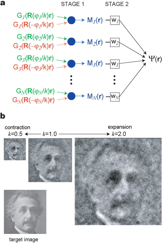
Scale-invariant representation of a visual image by moiré grids. a, Two-stage model for constructing image representations. b, The target image was a 272 × 272 pixel grayscale image (bottom left). Weighting coefficients for a basis set of 1500 grid fields were fit to the target image with k = 1.0. Then, a half-sized image was produced by setting k = 0.5, and a double-sized image was produced by setting k = 2.0. In these simulations, moiré grids were constructed using the rotational scaling rule, and the k parameter modulated the angle between the sibling grid pair that formed each moiré grid.
In the place cell simulations above, the population of moiré grids Mi(r) was produced from pairs of theta grids using the length scaling rule (Fig. 6a, first stage of the two-stage model), which we believe corresponds to the manner in which layer II grid cells are formed in dMEC (Fig. 4). In the visual image simulations presented below, the population of moiré grids Mi(r) was instead produced from pairs of theta grids using the rotational scaling rule (Fig. 10, first stage of the two-stage model at top right), which we believe corresponds to the manner in which layer III grid cells are formed in dMEC (Fig. 5). We used different scaling rules for the place field and visual image simulations merely to demonstrate that both the length and rotational scaling rules are capable of producing scale-invariant memory representations.
To implement uniform rescaling of a population of moiré grids Mi(r) produced by the rotational scaling rule, it is necessary to modify Equation 13 by inserting a scaling factor k. This can be achieved by substituting angle ϕi with ϕi/k to obtain the following:
 |
where all terms other than k are identical to those in Equation 13 above. The substitution of ϕi with ϕi/k does not produce perfect rescaling of the moiré grids Mi(r) in unison with k, but only approximate rescaling (see Appendix B). To achieve perfect rescaling, ϕi must be replaced with a function much more complex than ϕi/k. However, for the simulations presented here, the approximation ϕi/k was sufficient to produce very good results, so we used ϕi/k for simplicity.
For visual image simulations, input to the model was provided by a population of “visual grid cells” that tiled the visual field with hexagonal lattices. To our knowledge, cells that tile the visual field with hexagonal grids have not yet been observed in neurophysiological studies of the visual system (although it is worth noting that the retina itself is a hexagonal lattice of photoreceptors). Thus, we cannot make any strong predictions about exactly which neurons in the brain might correspond to the visual grid cells in the image simulations presented here, other than to speculate that neurons with lattice-like receptive fields may exist in some parts of the visual pathway that are involved in storing scale-invariant memories of familiar images, possibly in entorhinal areas that are homologous to dMEC in rats.
The target function for visual image simulations was a grayscale picture of a face measuring 272 × 272 pixels (Fig. 10). To construct a memory of the target image out of grid fields, input to the first stage of the model was provided by 3000 theta grids, with each theta grid generated by the cosine grating model described in Materials and Methods. The theta grids were grouped into pairs that provided input to N = 1500 moiré grid cells, Mi(r), whose activity levels were computed using Equation 18. The vertex spacing length was identical (λ = 4.6 pixels) for all 3000 theta grids that provided input to the model. Hence, the vertex spacing of each Mi(r) was determined solely by the angle of rotation between the pair of theta grids that provided its input.
The vertex spacings Siλ of moiré grids Mi(r) were uniformly random in the range 15 < Siλ < 120 pixels; this distribution of vertex spacings for the moiré grids was achieved by randomly assigning the sibling grid counter-rotation angles to values in the range ϕmin < ϕi < ϕmax, where ϕmin = 2.2° and ϕmax = 17.7°. It may be verified that Siλ ranges between 15 and 120 pixels for these parameter choices by assigning λ = 4.6 pixels and substituting 2ϕmin or 2ϕmax for φ in the rotational scaling rule (Eq. 3); this produces Siλ between 15 and 120 pixels. The angular orientations of Mi(r) were uniformly random in the range 0° ≤ θi < 60°.
In the second stage of the model (Fig. 10, top right), the moiré grids Mi(r) were linearly summed using the following equation:
 |
where ψ(r) is the output of the model, which recalls a “memory” of the stored grayscale image. Unlike place cell simulations (Eq. 15), there was no thresholding of ψ(r) in the visual image simulations. The population of moiré grids, Mi(r), was assigned weighting coefficients wi using the pseudoinverse method (Eq. 16), as in place cell simulations above. Weights were chosen to obtain the optimal fit of the output of the model to the grayscale target image, from which the target vector t was derived. The scaling parameter was set to k = 1.0 while fitting the target image (Eq. 18). After the optimal weight coefficients had been computed, the output of the model, ψ(r), produced an image that clearly resembled the target image, as shown in Figure 10. The graininess in the output image is caused by the high spatial frequency of the input grids, just as the “speckles” in simulated place cell firing rate maps were produced by the high-frequency theta grids in place cell simulations above.
As in simulations with the place cell model, it was possible to rescale the entire output image simply by adjusting the scaling parameter k while the weighting coefficients wi remained fixed at constant values. Figure 10 shows a double-sized output image (544 × 544 pixels) that was produced by increasing the scaling factor to k = 2.0 and a half-sized image (136 × 136 pixels) that was produced by decreasing the scaling factor to k = 0.5. These simulations demonstrate that if a visual image is encoded as a linear combination of scalable moiré grids, then the image is automatically represented across infinite range of different sizes (the size range has a lower bound but no upper bound, as can be seen from the scaling functions illustrated in Figs. 2c and 3d). Even for very large basis sets that consist of thousands of grid cells (as in our visual image simulations), the scale of the stored image may be adjusted easily by setting only three parameters: the scaling parameter k and the x and y coordinates of the scaling origin.
Discussion
Here, we have shown that pairs of hexagonal grid fields can interfere with one another to form moiré grids that replicate themselves over a broad range of spatial scales. Grid cells in dMEC can be simulated as moiré grids that are formed by inputs from smaller theta grids (Figs. 2–5). Outputs from dMEC grid cells can be combined to form yet larger moiré grids, suggesting that grid cells with very large vertex spacings might be found downstream from dMEC grid cells in the rat brain. Outputs from dMEC grid cells can be summed to construct hippocampal place cells (Fig. 6), as shown in previous studies (McNaughton et al., 2006; Solstad et al., 2006). The scaling properties of moiré grids may help to explain how place cells rescale their firing fields when a familiar environment is resized (Figs. 7–9), and we have shown that a population of moiré grids can serve as a basis set for constructing size-invariant representations of visual images (Fig. 10). Based on these findings, we speculate that an important function of grid cells might be to generate scalable basis functions that can serve as building blocks for constructing size-invariant memory representations of familiar stimuli.
What is theta rhythm?
Movement-related theta oscillations have long been known to exist in the rat brain (Vanderwolf, 1969), and numerous theories have been proposed to explain the functional significance of theta rhythm (Buzsaki, 2005; Jensen and Lisman, 1996; Hasselmo and Eichenbaum, 2005). Here, we have proposed that movement-related theta rhythm is produced by small hexagonal grid fields that provide the elementary building blocks from which scale-invariant memory representations are formed. Our model can be regarded as an extension of previous dual oscillator models, which explain phase precession by place cells and grid cells as a phenomenon that emerges from interference between sinusoids (O'Keefe and Recce, 1993; Lengyel et al., 2003; O'Keefe and Burgess, 2005). Like these previous models, our theory also explains phase precession (as well as spatial tuning of place cells and grid cells) by interference between periodic signals, but here the periodic signals are planar grids rather than linear sinusoids (Burgess et al., 2005).
O'Keefe and Burgess (2005) observed that the periodicity of dMEC grids is similar to the periodicity of sinusoidal elements that comprise dual oscillator models, and they predicted that dMEC grid cells might therefore exhibit phase precession as the rat traverses each vertex of a dMEC grid. This prediction was later confirmed by data showing that grid cells in layer II of dMEC exhibit phase precession (Hafting et al., 2006). In our model, this phase precession was explained by the length scaling rule (Eq. 2), which can be regarded as a planar extension of the dual oscillator theory (Fig. 4). However, it has also been reported that some dMEC grid cells, especially in layer III, do not exhibit theta phase precession (Hafting et al., 2006). To account for these findings, our model hypothesizes that some dMEC grids might be formed from theta grids that differ in their angular orientation rather than their vertex spacing (see the rotational scaling rule, Equation 3). This novel hypothesis generates an experimentally testable prediction that some grid cells should exhibit a previously unobserved form of lateral phase shifting along the dimension perpendicular to the rat's direction of travel (rather than parallel to the direction of travel, as in classical phase precession). Thus, as a rat passes through each vertex of a dMEC grid formed by rotational scaling, the grid cell should fire at a phase of theta rhythm that depends on the rat's lateral position within the vertex (Fig. 5). Such lateral phase shifting would only be observable in a two-dimensional environment (an open field but not a linear track), because it requires a degree of freedom along the dimension perpendicular to the rat's direction of travel. Some dMEC grids might be formed from theta grids that differ in both their vertex spacing and angular orientation (see the generalized scaling rule of Equation 5), and these cells would simultaneously exhibit standard phase precession and lateral phase shifting.
Attractor–integrator networks for producing theta grids
To reconcile the fact that dMEC grids have stable vertex spacings with the fact that the frequency of theta rhythm is nearly constant at different running speeds, our model proposes that the vertex spacing of theta grids changes systematically with running speed. It is therefore incumbent on our theory to propose a biological mechanism for generating theta grids with speed-dependent vertex spacings.
It has been hypothesized that grid cell firing fields in dMEC are produced by an attractor network that performs path integration of the rat's movements through its environment (O'Keefe and Burgess, 2005; Fuhs and Touretzky, 2006; McNaughton et al., 2006). Here, we have proposed an alternative hypothesis, that dMEC grids are formed by moiré interference between theta grids. However, theta grids might be generated by the same type of attractor–integrator network that has previously been proposed to generate dMEC grids, except that the grid fields produced by the path integrator would be smaller than previously assumed, and their vertex spacings would vary with running speed to keep the frequency of theta rhythm constant. The vertex spacing of theta grids formed by such a path integration network would depend on the gain function of the velocity input to the integrator (Maurer et al., 2005; McNaughton et al., 2006). A unity gain function would be required to produce theta grids with constant vertex spacings; any other gain function would produce theta grids with variable vertex spacings. Hence, it is not at all unreasonable to propose that a path integration network might produce grid fields with variable vertex spacings. Our model specifically proposes that the gain function of the velocity input obeys relationships similar to Equations 8 and 9 (or, alternatively, mechanisms outlined in Appendix A), so that moiré grids formed from theta grids will have constant vertex spacings at all running speeds.
Where might the theta grid path integrator reside in the rat brain? Production and synchronization of theta rhythm involves an ascending pathway from the brainstem to the mammillary nuclei, which then ascends through the medial septum and diagonal band to reach the hippocampus and limbic cortex (Vertes and Kocsis, 1997; Pan and McNaughton, 2002). Hence, the mammillary complex seems well positioned to contain a theta path integration network, because it receives afferent inputs from brainstem and vestibular nuclei that encode velocity information (Shibata, 1987; Gonzalo-Ruiz et al., 1992) and sends efferent outputs to the septohippocampal system that participate in regulating theta oscillations. Interestingly, the lateral mammillary nuclei appear to contain critical components of an attractor network that performs path integration of head-turning movements to produce head-direction cells (Sharp et al., 2001). Neighboring circuits in the medial and supramammillary nuclei might thus contain similar path integration networks for producing theta grids, which might explain why these areas play an important role in generating the theta rhythm.
Grid field rescaling
Our model of place field rescaling (Figs. 7, 8) predicts that when a familiar environment is resized, moiré grid cells should rescale their grid spacings along with the size of the environment (Fig. 9). However, contradicting this prediction, Hafting et al. (2005) have reported that grid cells in layer II of dMEC did not rescale their grid fields when rats were moved back and forth between large- (2 m) and small (1 m)-diameter cylinders with similar visual features. Instead, layer II dMEC grid cells maintained the same vertex spacing in both cylinders. However, layer III grid cells were not recorded during these rescaling experiments, and because grid cells in layers II and III have significantly different firing properties (Hafting et al., 2006; Sargolini et al., 2006a), it is possible that layer III grid cells might show a stronger tendency than layer II cells to rescale their grid fields when the size of the cylinder is altered. Indeed, recent experiments have reported that manipulations of the environment can in fact cause changes in the vertex spacing of grid cells in layer III of dMEC (Fyhn et al., 2006). It has also been reported that grid cells exist in other areas of the rat brain in addition to dMEC (Sargolini et al., 2006b). If the rat brain contains diverse grid cell populations residing in different cortical layers and different anatomical regions, then some of these populations may rescale their firing fields when an environment is resized (as in our simulations), whereas other populations might maintain fixed vertex spacings that do not rescale with the environment (as reported by Hafting et al., 2005). In this way, different grid cell populations might offer competing interpretations of the same spatial environment to the hippocampal network. Our model strongly predicts that some subpopulations of grid cells should rescale in unison when a familiar environment is resized (Fig. 9), but the model does not predict that all grid cells must behave in this manner, so the findings of Hafting et al. (2005) do not strongly contradict the predictions of the model.
Appendix
A. Constant dMEC grid spacings from speed-dependent theta grid orientations
Moiré grids with constant vertex spacing can be constructed from two theta grids with speed-varying vertex spacings. Equation 9 provides a way to do this in the special case in which the two theta grids have identical orientations and different vertex spacings. In the opposite case, in which the theta grids differ in their angular orientation but not their vertex spacings, a constant moiré grid spacing can be achieved if the angle between the theta grids varies systematically with running speed. Suppose a moiré grid is produced by interference between two theta grids, G1 and G2, which have identical speed-dependent vertex spacings λ(V). If λ(V) = V/f, then theta oscillations produced by G1 and G2 will have the same frequency f at all running speeds (similar to Eq. 8). Now suppose that G1 and G2 have different angular orientations, denoted θ1(V) and θ2(V), which also depend on running speed. The difference in angular orientations between the theta grids may be denoted as φ(V) = |θ1(V) − θ2(V)|. The vertex spacing of the moiré grid will be Sλ(V), where the scaling factor S is given by the rotational scaling rule (Eq. 3). Although the theta grid vertex spacings and orientations change with running speed, it can be shown algebraically from Equation 3 that the moiré grid vertex spacing remains constant at all running speeds as long as the following is true:
 |
where λM is the fixed vertex spacing of the moiré grid, and f is the frequency of theta rhythm produced by vertex crossings on G1 and G2. Hence, the moiré grid can maintain a stable vertex spacing if the angular orientation between the theta grids varies with running speed in accordance with Equation 20. It is difficult to envision a biologically plausible mechanism for rotating theta grids as a function of running speed, so solutions that involve changing the relative grid spacings (as in Eq. 9) may be preferable to those that involve changing the relative grid orientation (as in Eq. 20).
B. Approximate rescaling moiré grids by a divisive scaling factor
For moiré grids constructed by the length scaling rule, k divisively modifies αi, which is the difference between vertex spacings of the theta grid pair (Eq. 17). To see how changing k will alter the vertex spacing of a moiré grid constructed from theta grids, we may replace αi with αi/k in the length scaling rule of Equation 2 to obtain the following:
 |
where superscript k is added to Si on the left side to emphasize the dependence on k. Now, we can express the proportional change in S when k is modified:
 |
Hence, S scales approximately in proportion with k, so that k multiplicatively modifies the moiré grid spacings. The approximation step in Equation 22 is only valid when αi is small (that is, when 0 < αi ≪ 1), a condition which holds well enough in our place cell simulations to produce good rescaling results (Fig. 7c, 8c).
For moiré grids constructed by the rotational scaling rule, k modifies the angle between theta grids (Eq. 18) so that when the value of k is changed, all of the counter-rotation angles ϕi change by the same factor. Then, the final output of the model in Equation 15 or 19 also changes its size by approximately the same factor. To see why this method works, setting φ = 2ϕi/k in Equation 3 yields the following moiré scaling factor:
 |
where superscript k is again introduced to emphasize the dependence on k. It can be shown algebraically that the following is true:
 |
Notice that by this equation, Sik/Sik=1 ≈ k when the angle ϕi is small, because sin x ≈ x for small x. Thus, as long as a theta grid pair starts out with a small counter-rotation angle ϕi before rescaling (when k = 1), the spacing of a moiré grid constructed from the theta grids will scale by a factor approximately equal to k (specifically, Sik/Sik=1 ≈ k) when k is adjusted. The approximation is good enough in our visual image simulations to produce a rescaled image (Fig. 10).
Footnotes
This work was supported by National Institutes of Health Grant R01MH079511-02 awarded to H.T.B. and K.Z. through the National Science Foundation Collaborative Research in Computational Neuroscience funding initiative.
We thank Frank Krasne, Josh Johansen, Jason Tarpley, Tom Blair, Torkel Hafting, Marianne Fyhn, Alessandro Treves, Edvard Moser, Trygve Solstad, Neil Burgess, and three anonymous reviewers for helpful comments and discussion. We thank Mark Strohm, Adam Aron, and Russ Poldrack for technical computing assistance.
References
- Amidror I. The theory of the moiré phenomenon. Kluwer Academic; 2000. [Google Scholar]
- Barry C, Lever C, Hayman R, Hartley T, Burton S, O'Keefe J, Jeffery K, Burgess N. The boundary vector cell model of place cell firing and spatial memory. Rev Neurosci. 2006;17:71–97. doi: 10.1515/revneuro.2006.17.1-2.71. [DOI] [PMC free article] [PubMed] [Google Scholar]
- Biederman I, Cooper EE. Size invariance in visual object priming. J Exp Psychol Hum Percept Perform. 1992;18:121–133. [Google Scholar]
- Brown MW, Aggleton JP. Recognition memory: what are the roles of the perirhinal cortex and hippocampus? Nat Rev Neurosci. 2001;2:51–61. doi: 10.1038/35049064. [DOI] [PubMed] [Google Scholar]
- Burgess N, Barry C, Jefferies KJ, O'Keefe J. A grid and place cell model of path integration utilizing phase precession versus theta. 1st Annual Conference on Computational Cognitive Neuroscience; Washington, DC. 2005. [Google Scholar]
- Buzsaki G. Theta rhythm of navigation: link between path integration and landmark navigation, episodic and semantic memory. Hippocampus. 2005;15:827–840. doi: 10.1002/hipo.20113. [DOI] [PubMed] [Google Scholar]
- Eichenbaum H. Hippocampus: cognitive processes and neural representations that underlie declarative memory. Neuron. 2004;44:109–120. doi: 10.1016/j.neuron.2004.08.028. [DOI] [PubMed] [Google Scholar]
- Fried I, MacDonald KA, Wilson C. Single neuron activity in human hippocampus and amygdale during recognition of faces and objects. Neuron. 1997;18:753–765. doi: 10.1016/s0896-6273(00)80315-3. [DOI] [PubMed] [Google Scholar]
- Fuhs MC, Touretzky DS. A spin glass model of path integration in rat medial entorhinal cortex. J Neurosci. 2006;26:4266–4276. doi: 10.1523/JNEUROSCI.4353-05.2006. [DOI] [PMC free article] [PubMed] [Google Scholar]
- Fyhn M, Molden S, Witter MP, Moser EI, Moser MB. Spatial representation in the entorhinal cortex. Science. 2004;305:1258–1264. doi: 10.1126/science.1099901. [DOI] [PubMed] [Google Scholar]
- Fyhn MH, Hafting TF, Treves A, Moser EI, Moser MB. Coherence in ensembles of entorhinal grid cells. Soc Neurosci Abstr. 2006;32:68–9. [Google Scholar]
- Gonzalo-Ruiz A, Alonso A, Sanz JM, Llinas RR. Afferent projections to the mammillary complex of the rat, with special reference to those from surrounding hypothalamic regions. J Comp Neurol. 1992;321:277–299. doi: 10.1002/cne.903210208. [DOI] [PubMed] [Google Scholar]
- Hafting T, Fyhn M, Molden S, Moser MB, Moser EI. Microstructure of a spatial map in the entorhinal cortex. Nature. 2005;436:801–806. doi: 10.1038/nature03721. [DOI] [PubMed] [Google Scholar]
- Hafting T, Fyhn MH, Moser MB, Moser EI. Phase precession and phase locking in entorhinal grid cells. Soc Neurosci Abstr. 2006;32:68–8. [Google Scholar]
- Hartley T, Burgess N, Lever C, Cacucci F, O'Keefe J. Modeling place fields in terms of the cortical inputs to the hippocampus. Hippocampus. 2000;10:369–379. doi: 10.1002/1098-1063(2000)10:4<369::AID-HIPO3>3.0.CO;2-0. [DOI] [PubMed] [Google Scholar]
- Hasselmo ME, Eichenbaum H. Hippocampal mechanisms for the context-dependent retrieval of episodes. Neural Netw. 2005;18:1172–1190. doi: 10.1016/j.neunet.2005.08.007. [DOI] [PMC free article] [PubMed] [Google Scholar]
- Huxter J, Burgess N, O'Keefe J. Independent rate and temporal coding in hippocampal pyramidal cells. Nature. 2003;425:828–832. doi: 10.1038/nature02058. [DOI] [PMC free article] [PubMed] [Google Scholar]
- Jensen O, Lisman JE. Novel lists of 7 +/− 2 known items can be reliably stored in an oscillatory short-term memory network: interaction with long-term memory. Learn Mem. 1996;3:257–263. doi: 10.1101/lm.3.2-3.257. [DOI] [PubMed] [Google Scholar]
- Jolicoeur P. A size-congruency effect in memory for visual shape. Mem Cogn. 1987;15:531–543. doi: 10.3758/bf03198388. [DOI] [PubMed] [Google Scholar]
- Kreiman G, Koch C, Fried I. Imagery neurons in the human brain. Nature. 2000;408:357–361. doi: 10.1038/35042575. [DOI] [PubMed] [Google Scholar]
- Lengyel M, Szatmary Z, Erdi P. Dynamically detuned oscillations account for the coupled rate and temporal code of place cell firing. Hippocampus. 2003;13:700–714. doi: 10.1002/hipo.10116. [DOI] [PubMed] [Google Scholar]
- Manns JR, Hopkins RO, Reed JM, Kitchener EG, Squire LR. Recognition memory and the human hippocampus. Neuron. 2003;37:171–180. doi: 10.1016/s0896-6273(02)01147-9. [DOI] [PubMed] [Google Scholar]
- Maurer AP, Vanrhoads SR, Sutherland GR, Lipa P, McNaughton BL. Self-motion and the origin of differential spatial scaling along the septo-temporal axis of the hippocampus. Hippocampus. 2005;15:841–852. doi: 10.1002/hipo.20114. [DOI] [PubMed] [Google Scholar]
- Maurer AP, Cowen SL, Burke SN, Barnes CA, McNaughton BL. Organization of hippocampal cell assemblies based on theta phase precession. Hippocampus. 2006;16:785–794. doi: 10.1002/hipo.20202. [DOI] [PubMed] [Google Scholar]
- McNaughton BL, Battaglia FP, Jensen O, Moser EI, Moser MB. Path integration and the neural basis of the ‘cognitive map.'. Nat Rev Neurosci. 2006;7:663–678. doi: 10.1038/nrn1932. [DOI] [PubMed] [Google Scholar]
- Mitchell SJ, Ranck JB., Jr Generation of theta rhythm in medial entorhinal cortex of freely moving rats. Brain Res. 1980;189:49–66. doi: 10.1016/0006-8993(80)90006-2. [DOI] [PubMed] [Google Scholar]
- Moita MAP, Rosis S, Zhou Y, LeDoux JE, Blair HT. Putting fear in its place: remapping of hippocampal place cells during fear conditioning. J Neurosci. 2004;24:7015–7023. doi: 10.1523/JNEUROSCI.5492-03.2004. [DOI] [PMC free article] [PubMed] [Google Scholar]
- Muller RU, Kubie JL. The effects of changes in the environment on the spatial firing of hippocampal complex-spike cells. J Neurosci. 1987;7:1951–1968. doi: 10.1523/JNEUROSCI.07-07-01951.1987. [DOI] [PMC free article] [PubMed] [Google Scholar]
- Nishijima Y, Oster G. Moiré patterns: their application to refractive index and refractive index gradient measurements. J Opt Soc Am. 1964;54:1–5. [Google Scholar]
- O'Keefe J, Burgess N. Geometric determinants of the place fields of hippocampal neurons. Nature. 1996;381:425–428. doi: 10.1038/381425a0. [DOI] [PubMed] [Google Scholar]
- O'Keefe J, Burgess N. Dual phase and rate coding in hippocampal place cells: theoretical significance and relationship to entorhinal grid cells. Hippocampus. 2005;15:853–866. doi: 10.1002/hipo.20115. [DOI] [PMC free article] [PubMed] [Google Scholar]
- O'Keefe J, Dostrovsky J. The hippocampus as a spatial map. Preliminary evidence from unit activity in the freely-moving rat. Brain Res. 1971;34:171–175. doi: 10.1016/0006-8993(71)90358-1. [DOI] [PubMed] [Google Scholar]
- O'Keefe J, Nadel L. The hippocampus as a cognitive map. Oxford UP: Oxford; 1978. [Google Scholar]
- O'Keefe J, Recce MR. Phase relationship between hippocampal place units and the EEG theta rhythm. Hippocampus. 1993;3:317–330. doi: 10.1002/hipo.450030307. [DOI] [PubMed] [Google Scholar]
- Oster G. The science of moiré patterns. Tonawanda, NY: Edmund Scientific; 1969. [Google Scholar]
- Pan WX, McNaughton N. The role of the medial supramammillary nucleus in the control of hippocampal theta activity and behaviour in rats. Eur J Neurosci. 2002;16:1797–1809. doi: 10.1046/j.1460-9568.2002.02267.x. [DOI] [PubMed] [Google Scholar]
- Quiroga RQ, Reddy L, Kreiman G, Koch C, Fried I. Invariant visual representation by single neurons in the human brain. Nature. 2005;435:1102–1107. doi: 10.1038/nature03687. [DOI] [PubMed] [Google Scholar]
- Rivas J, Gaztelu JM, Garcia-Austt E. Changes in hippocampal cell discharge patterns and theta rhythm spectral properties as a function of walking velocity in the guinea pig. Exp Brain Res. 1996;108:113–118. doi: 10.1007/BF00242908. [DOI] [PubMed] [Google Scholar]
- Samsonovich A, McNaughton B. Path integration and cognitive mapping in a continuous attractor neural network model. J Neurosci. 1997;17:5900–5920. doi: 10.1523/JNEUROSCI.17-15-05900.1997. [DOI] [PMC free article] [PubMed] [Google Scholar]
- Sargolini F, Fyhn M, Hafting T, McNaughton BL, Witter MP, Moser MB, Moser EI. Conjunctive representation of position, direction, and velocity in entorhinal cortex. Science. 2006a;312:758–762. doi: 10.1126/science.1125572. [DOI] [PubMed] [Google Scholar]
- Sargolini F, Boccara C, Witter MP, Moser MB, Moser EI. Grid cells outside the medial entorhinal cortex. Soc Neurosci Abstr. 2006b;32:68–11. [Google Scholar]
- Sharp PE. Subicular place cells expand or contract their spatial firing pattern to fit the size of the environment in an open field but not in the presence of barriers: comparison with hippocampal place cells. Behav Neurosci. 1999;113:643–663. doi: 10.1037//0735-7044.113.4.643. [DOI] [PubMed] [Google Scholar]
- Sharp PE, Blair HT, Cho J. The anatomical and computational basis of the rat head-direction cell signal. Trends Neurosci. 2001;24:289–294. doi: 10.1016/s0166-2236(00)01797-5. [DOI] [PubMed] [Google Scholar]
- Shibata H. Ascending projections to the mammillary nuclei in the rat: a study using retrograde and anterograde transport of wheat germ agglutinin conjugated to horseradish peroxidase. J Comp Neurol. 1987;264:205–215. doi: 10.1002/cne.902640206. [DOI] [PubMed] [Google Scholar]
- Skaggs WE, Knierim JJ, Kudrimoti HS, McNaughton BL. A model of the neural basis of the rat's sense of direction. In: Tesauro G, Touretzky D, Leen T, editors. Advances in neural information processing systems. Vol 7. Cambridge, MA: Massachusetts Institute of Technology; 1995. [PubMed] [Google Scholar]
- Skaggs WE, McNaughton BL, Wilson MA, Barnes CA. Theta phase precession in hippocampal neuronal populations and the compression of temporal sequences. Hippocampus. 1996;6:149–172. doi: 10.1002/(SICI)1098-1063(1996)6:2<149::AID-HIPO6>3.0.CO;2-K. [DOI] [PubMed] [Google Scholar]
- Solstad T, Moser EI, Einevoll GT. From grid cells to place cells: a mathematical model. Hippocampus. 2006;16:1026–1031. doi: 10.1002/hipo.20244. [DOI] [PubMed] [Google Scholar]
- Squire LR, Stark CE, Clark RE. The medial temporal lobe. Annu Rev Neurosci. 2004;27:279–306. doi: 10.1146/annurev.neuro.27.070203.144130. [DOI] [PubMed] [Google Scholar]
- Stark CE, Squire LR. Functional magnetic resonance imaging (fMRI) activity in the hippocampal region during recognition memory. J Neurosci. 2000;20:7776–7781. doi: 10.1523/JNEUROSCI.20-20-07776.2000. [DOI] [PMC free article] [PubMed] [Google Scholar]
- Stecher M. The moiré phenomenon. Am J Phys. 1964;32:247–257. [Google Scholar]
- Thompson LT, Best PJ. Long-term stability of the place-field activity of single units recorded from the dorsal hippocampus of freely behaving rats. Brain Res. 1990;509:299–308. doi: 10.1016/0006-8993(90)90555-p. [DOI] [PubMed] [Google Scholar]
- Vanderwolf CH. Hippocampal electrical activity and voluntary movement in the rat. Electroencephalogr Clin Neurophysiol. 1969;26:407–418. doi: 10.1016/0013-4694(69)90092-3. [DOI] [PubMed] [Google Scholar]
- Vertes RP, Kocsis B. Brainstem-diencephalo-septohippocampal systems controlling the theta rhythm of the hippocampus. Neuroscience. 1997;81:893–926. doi: 10.1016/s0306-4522(97)00239-x. [DOI] [PubMed] [Google Scholar]
- Whishaw IQ, Vanderwolf CH. Hippocampal EEG, behavior: changes in amplitude and frequency of RSA (theta rhythm) associated with spontaneous and learned movement patterns in rats and cats. Behav Biol. 1973;8:461–484. doi: 10.1016/s0091-6773(73)80041-0. [DOI] [PubMed] [Google Scholar]
- Wilson MA, McNaughton BL. Dynamics of the hippocampal ensemble code for space. Science. 1993;261:1055–1058. doi: 10.1126/science.8351520. [DOI] [PubMed] [Google Scholar]