

Abstract
Several behavioral experiments suggest that the nervous system uses an internal model of the dynamics of the body to implement a close approximation to a Kalman filter. This filter can be used to perform a variety of tasks nearly optimally, such as predicting the sensory consequence of motor action, integrating sensory and body posture signals, and computing motor commands. We propose that the neural implementation of this Kalman filter involves recurrent basis function networks with attractor dynamics, a kind of architecture that can be readily mapped onto cortical circuits. In such networks, the tuning curves to variables such as arm velocity are remarkably noninvariant in the sense that the amplitude and width of the tuning curves of a given neuron can vary greatly depending on other variables such as the position of the arm or the reliability of the sensory feedback. This property could explain some puzzling properties of tuning curves in the motor and premotor cortex, and it leads to several new predictions.
Keywords: sensorimotor integration, Kalman filter, motor control, population code, line attractors, basis functions
Introduction
Fast and accurate behavior requires the integration of multiple sources of sensory and motor signals. For example, to hit a tennis ball, a player must take into account the position and motion of the ball, as well as his own position and movements. Estimating these variables in real time is difficult because of the presence of noise in the sensory receptors, motor effectors (Schmidt et al., 1979; Slifkin and Newell, 1999; Jones et al., 2002), and cortical circuits (Tolhurst et al., 1982; Vogels et al., 1989; Shadlen and Newsome, 1994; Riehle et al., 1997; Lee et al., 1998). This noise could be filtered out through simple averaging, either over time or space, but several factors make this averaging difficult.
The first problem comes from the format of the neural code. Sensory and motor variables in the cortex are often encoded with population codes, i.e., noisy hills of activity generated by a large number of neurons with overlapping bell-shaped tuning curves (Georgopoulos et al., 1982; Lee et al., 1988; Zohary, 1992) (see Fig. 1). Averaging the neural responses over the entire population would recover a number unrelated to the direction of motion. Clearly, the position of the hill on the neuronal array conveys some information about direction, but, as we will see, more complex decoding techniques are required to recover this information.
Figure 1.

Optimal estimation of noisy population codes by recurrent networks. A, Tuning curves of a model population of medial temporal (MT) neurons to direction of motion. B, Average activity of MT cells as a function of their preferred direction when presented with a motion x = 0°. C, Population activity (spike counts) on a given trial. Spike counts are drawn from a Poisson distribution with rates specified by the mean activities shown in B. D, Stable state of a line-attractor recurrent network when initialized with the activity pattern in C. With appropriate tuning of the lateral connection, the position of the peak activity x̂ is within 5% of the maximum-likelihood estimate of motion direction given the noisy neural responses shown in C.
A second problem with averaging, and in particular with temporal averaging, is that sensory and motor variables tend to change rapidly over time in realistic situations. For example, humans move their eyes three to four times per second, limiting the effective temporal averaging to a maximum of ∼250–350 ms (Ballard et al., 2000). This does not entail that temporal averaging is impossible. If the amplitude and direction of the eye movement is known, the image changes in a predictable way. Therefore, it is possible to average, or integrate, information across saccades, but this requires an internal model of how sensory inputs are modified as a result of a motor action. Recent psychophysics experiments strongly suggest that such internal models are used by the nervous system for estimating sensory variables and for optimal motor control (Wolpert et al., 1995a; Kawato, 1999; Desmurget and Grafton, 2000; Mehta and Schaal, 2002; Todorov, 2004; Saunders and Knill, 2005), but very little is known about the neural implementation of these internal models.
When the internal model is linear and the noise is Gaussian, the optimal strategy for combining sensory inputs and the predictions of the internal model is known as a Kalman filter. Kalman filters can be used for optimal motor control and are also at the heart of recent models of decision making (Gold and Shadlen, 2003; Dorris and Glimcher, 2004; Sugrue et al., 2004) and classical conditioning (Dayan and Balleine, 2002). This study shows how a particular class of neural network, known as recurrent basis function networks, can implement the internal model and the Kalman filter. We start by demonstrating the optimality of our approach on a simple problem: locating the position of an object while moving the eyes. We then move on to a problem requiring a complex internal model, namely, locating the position of one's arm. We end by showing that our model behaves in a way consistent with what has been observed with human subjects engaged in the same “task,” and we discuss experimental predictions for single-cell recordings.
Materials and Methods
This section is divided into two parts. The first part (Intuitive description of the approach) contains no equations and describes, in relatively simple terms, the concepts of Kalman filters and attractor networks. The second part (Formalization) contains the equations and parameter settings necessary to reproduce our results.
Intuitive description of the approach
For a concrete example, consider the problem of localizing one's arm during a movement in complete darkness, i.e., without visual feedback. The trajectory of the arm can be inferred from two independent sources of information: the noisy proprioceptive feedback encoding arm position and velocity and the prediction generated by the internal model of arm dynamics. In this case, the internal model is a model that predicts where the arm should be given the position of the arm at the previous time step and the motor command issued to the arm at the last time step.
If the internal model is linear and the noise is Gaussian, the optimal way to combine those signals is to use a Kalman filter (Anderson and Moore, 1979). A Kalman filter is an optimal integrator in the sense that it minimizes the mean square error of the estimate, given the full history of sensory feedback received during the movement. The key property of a Kalman filter is its ability to combine internally generated estimates with estimates obtained from sensory feedback.
In our previous work (Deneve et al., 1999, 2001), we showed how to perform optimal estimation and combination in neural networks using noisy population codes. Figure 1D illustrates the solution we had devised for estimating optimally the value of a variable given a noisy hill of activity. The basic idea is to use an attractor network in which the population activity stabilizes over time onto smooth hills of activity. When initialized with a noisy hill of activity, the network settles onto a smooth hill whose position can be interpreted as an estimate of the variable encoded in the noisy hill. The mean and variance of this estimate can be computed numerically by repeating the simulation many times, using the same direction of motion but different instantiation of the noise on each trial. For Poisson noise, we have shown that the position of the smooth hill provides a close approximation to a maximum-likelihood estimate. The maximum-likelihood estimate is optimal in the sense that it is “unbiased” and has near-minimal variance. The term unbiased means that the estimate is equal to the true value of direction on average. If this is the case, the accuracy of the estimate is controlled by its variance. Given the noise corrupting the data, the variance is bounded below by what is known at the Cramer–Rao bound, which is the smallest achievable variance (Papoulis, 1991). With proper tuning of the weights, we reported that our network estimate has a variance within 5% of the Cramer–Rao bound (Deneve et al., 1999).
This example concerns only one population code for one scalar variable, but we have shown that a similar approach can be used to combine optimally variables encoded in multiple population codes, as long as these variables are functionally related (Deneve et al., 2001; Pouget et al., 2002; Deneve, 2004). For instance, we have simulated a network that can combine optimally a population code for the position on an object in visual coordinates and another one for the position of the same object in auditory coordinates. The network is initialized with those two population codes and computes a close approximation to the maximum-likelihood location of the stimulus given these inputs (Deneve et al., 2001).
The problem we are addressing now is similar. Instead of combining two population codes corresponding to two different sensory modalities, we want to combine one sensory population code with an internally generated population code corresponding to the estimate of the internal model. There are, however, some major differences. First, we are dealing now with continuous time-varying inputs. Our previous solution dealt only with static signals. With a continuous time-varying input, the network cannot stabilize onto a static smooth hill of activity because it is continuously perturbed by new inputs. Second, all of our previous work assumed independent Poisson noise. This assumption is clearly wrong for the internal model estimate. This estimate is the result of a computation. Any computation in a neural network involves an exchange of information among neurons, which creates correlations.
Despite those differences, we found that the same kind of attractor network can deal with time varying signals and can implement a close approximation to a Kalman filter. This new type of attractor network relies on a layer of sensorimotor units tuned to sensory variables and gain modulated by motor commands. Recurrent connections within this layer predict the future sensorimotor state given its current state and the efferent motor commands. Because sensorimotor tuning curves implement basis functions for sensory and motor variables, any dynamics over these variables can be approximated by such a network. In particular, connections can be set up so that the pattern of activity on the layers shifts and predicts the response of each unit at time t + dt, given the motor commands and the pattern of activity at time t. Thus, the sensorimotor units anticipate their future responses after the movement, implementing an internal model of the motor plant. The network connections also clean up the noise in the sensory inputs, preventing information loss through saturation while tracking the state of the sensorimotor system over time.
In addition, the networks can combine these internal estimates with on-line sensory feedback according to the respective reliabilities of these two signals. Our simulations demonstrate that these networks can be tuned to implement optimal Kalman filters and thus compute the most accurate on-line estimate for sensory and motor variables. These results are confirmed analytically in Materials and Methods and supplemental material (available at www.jneurosci.org).
Mathematical formalization
The estimation problem.
We consider a state vector of D temporally varying sensory variables x(t) = [xd(t)[ i = 1… D (D = 1 for object tracking, D = 2 for arm tracking) whose trajectories are controlled by a set of C motor commands c(t) = [ci(t)[ i = 1… C (C = 0 for object tracking, C = 1 for arm tracking) according to the following dynamical equation (boldface indicates vectors or matrices):
where M and B are matrices describing the sensorimotor dynamics: M = 1, Bc(t) = a = 0.003 in the object tracking example, and
 |
in the arm example. ε(t) is a white motor noise with a fixed covariance matrix Z. Z = 0.001 in the object tracking example, and
 |
for the arm example.
The sensory variables are never observed directly but must be inferred from noisy sensory feedbacks in the form of D noisy population codes:
fd is a P-dimensional vector representing the mean activity of a population of P neurons responding to variable xd(t). Nd is the neural noise, with covariance matrix Rd(t) = 〈Nd(t)Nd(t)〉. We assume that the noise is independent between the sensory inputs from different modality, i.e., 〈Nd(t)Nl(t)〉 = 0 for d ≠ l. The task is to find the most probable state of the system at time t, given the sensory inputs and the motor commands in the past:
 |
Scalar feedback estimates for sensory variables, x̂sd(t), can be obtained from the noisy population codes alone using maximum-likelihood estimation, defined as the value of xd(t) maximizing the probability of observing the sensory responses at time t:
 |
For large number of neurons, with Gaussian or Poisson noise, these estimates are unbiased and are the most accurate given the sensory noise (Brunel and Nadal, 1998).
For large number of neurons, because of the law of large numbers, the feedback estimates x̂s (t) = [x̂sd(t)]d = 1… D follow Gaussian distributions with mean x(t) and diagonal covariance matrix Q. The diagonal elements of this covariance matrix are the Cramer–Rao bounds computed from the covariance of the neural noise and the shape of the tuning curves:
 |
where
 |
is a vector of the partial derivative of the tuning curves with respect to xd, and Rd is the covariance matrix of the neuronal noise (Pouget et al., 1998).
Kalman filter solution.
In a Kalman filter, the maximum a posteriori estimate is given by the the following recursive equation:
where K(t) is the Kalman gain matrix. K(t) is computed iteratively according to the following:
 |
Σ(t) is the covariance of the Kalman filter estimates, and Σ(0) is the covariance of the prior on the initial state (Anderson and Moore, 1979). If the initial state is unknown, this variance is infinite.
We used Equations 6 and 7 to compute the optimal performance as predicted by a Kalman filter.
Network solution.
The network contains D sensory input layers and C motor input layers connecting a basis function layer of neurons [D = 1, C = 0 for object tracking; D = 2, C = 1 for arm tracking in one dimension (1D), and D = 4, C = 2 for arm tracking in two dimensions (2D)]. All input layers are one-dimensional layers of 20 neurons with bell-shaped tuning curves to either the sensory or the motor variables. The average activity of neurons i in sensory layer d with preferred value xid in response to input xd(t) is given by the following:
We considered that the sensory inputs xd(t) are periodic to avoid boundary effects and to ensure stability. This can be done without a loss of generality by assigning orientations close to ±180° to extreme sensory inputs which are never observed. The same equation with the same parameters was used to specify the tuning curves, fic(t), in the motor input layer.
The activity of the sensory unit i in layer d at time t, Sid(t) is drawn from a Poisson distribution:
 |
Motor input units are considered noiseless. Their activity is simply set to fic(t) at all times.
The basis function layer contained PC + D interconnected neurons (P = 60, D = 1, C = 0 for object tracking; P = 12, D = 2, C = 1 for arm localization in 1D; P = 6, D = 4, and C = 2 for arm localization in 2D). The activities of the basis function units are described by a PC + D dimensional vector, A(t). Each unit in this layer is characterized by a set of preferred sensory and motor states {cci, xid}c = 1… C,d = 1… D. Those preferred sensory and motor states form a regular grid of PC + D units covering 360° in all C + D dimensions. The activity of the basis function unit i at time t + 1 is updated according to the following:
 |
In this equation, and more generally in this section, Sid(t) refers to the input unit with preferred sensory state xid, where xid if the preferred sensory state for basis function unit i. The parameters λd(t) are the sensory gains (see Results for how they are adjusted over time). The motor command input, fic(t), modulates the gain of the basis function unit. In the object tracking example there is no motor command, and fic(t) = 1. The activation function h() implements a form of divisive normalization (Heeger, 1992a,b):
 |
The parameters μ and η were set to 0.001 and 0.01 for object tracking, and 0.001 and 0.005 for arm tracking. The lateral weights within the basis function layer, wijm, are given by the following:
 |
where xi = {cic, xid}c = 1… C,d = 1… D is the vector of preferred sensory state for unit i. L is a matrix describing the combined effect of M and B on the sensory and motor state vector xi. [Lxi]d is the dth component of the vector Lxi. The width of the weights, Kw, is computed to satisfy the condition for optimality described in supplemental material, available at www.jneurosci.org.
This bell-shaped pattern of weights is such that unit i is most strongly connected to the unit with preferred sensory state Lxi. This effectively implements the internal model by shifting the internal hill of activity within the basis function layer as specified by the state equation of the system (Eq. 1).
To optimize the network performance, that is, to bring the network performance as close as possible to the optimal performance predicted by a Kalman filter, the parameter Kw must be adjusted. This parameter controls the width of the weight pattern, and as a result, the width of the pattern of activity in the basis function layer. The optimal value can be inferred from our previous analytical work (Deneve et al., 2001; Latham et al., 2003). In both object and arm tracking, we obtained optimal performance for Kw equal to 3.
Convergence proof.
If we set the matrix L to the identity matrix in the equation that defines the lateral weights in the basis function layer (Eq. 12), the resulting set of equations is identical to the one we used in our previous work (Deneve et al., 2001). As a result, we know that if we initialize the network with noisy population codes and iterate the dynamical equations of the network, the activity in the basis function layer converges to a D-dimensional stable manifold. At this point, the activity in the basis function layer takes the form of a smooth hill of activity. If the network meets the condition derived by Latham et al. (2003), the position of this hill corresponds to the maximum-likelihood estimate of the sensory states encoded in the initial noisy sensory inputs. The condition derived by Latham et al. (2003) can be satisfied by tuning Kw, the width of the lateral weights.
If we now reinsert L in Equation 12 and initialize the network with noisy sensory inputs, the activity converges on a D-dimensional stable manifold, in the sense that the activity in the basis function layer converges toward a smooth hill. This smooth hill, however, moves over time with the dynamics specified by L. As a result, the position of the hill after t iterations reflects the maximum-likelihood estimate of the sensory states given the initial noisy sensory inputs after t iterations of the internal model. In other words, we obtain the estimate predicted by the internal model only.
To obtain a full Kalman filter, we need to add a mechanism to integrate the sensory feedback available at each time step. As shown in Equation 2, a linear operation is all we need, but the internal estimate and the sensory feedback must be weighted by the Kalman matrix for optimal performance. For how the Kalman gain was implemented, see below, Adjusting the sensory gain.
When the sensory feedback is added at every step, the activity in the basis function layer of the network, A(t), never stabilizes on the attractor (the D-dimensional manifold), which makes it more difficult to determine the estimate encoded by the network. We note, however, that at every time step, we know where the activity would stabilize if we were to stop the sensory feedback, and we were to replace the matrix L by the identity matrix in the lateral weights. It would stabilize onto a smooth hill peaking at the maximum-likelihood estimate of the sensory states given A(t). The position of this smooth hill can be read out with a simple center-of-mass estimate:
 |
Now that we have a network estimate at each time step, x̂N(t), we can compare its mean and variance to the mean and variance of the Kalman filter estimate. In Results, x̂N(t) was obtained through simulations. In the supplemental material (available at www.jneurosci.org), we show how to compute this estimate analytically in the limit of low noise. This approach allows us to determine the conditions under which the network is perfectly optimal.
Adjusting the sensory gains.
We update sensory gains according to the relative strength of sensory and internal signals, as in the Kalman filter equation:
 |
where qdd is the variance of the sensory estimates, and Σdd is derived from the Kalman filter equations. As long as sensory gains are adjusted accordingly and the condition for optimality derived by Deneve et al. (1999) and Latham et al. (2003) is verified, the network approximates the performance of a Kalman filter.
Results
A simple example: tracking a moving object
To illustrate our approach, we first consider a simple problem, namely, locating a static visual stimulus while the eyes are moving with speed −(a + ε)/δt, where a is a constant, and ε(t) is assumed to be white noise, i.e., it is drawn independently at each time step from a Gaussian distribution with mean 〈ε(t)〉 = 0 and constant variance. We assume that the neural circuits have knowledge of the average eye velocity (for instance, in the form of an efferent copy) but not of the noisy perturbation ε(t).
As a result of the eye movement, the horizontal position of the stimulus on the retina, denoted x(t), evolves according to the following:
We assume that the sensory feedback is provided by the response of a retinotopic map of neurons. At any given time, the object triggers a hill of activity centered at its current location. In the absence of noise, the hill follows a smooth Gaussian function as shown in Figure 2A. Neurons, however, are noisy, with noise following a near Poisson distribution (Vogels et al., 1989). For simplicity, we assume that the noise follows exactly a Poisson distribution, whose rate is specified by the smooth function shown in Figure 2A. On any given trial, the resulting activity over time takes the form of a succession of noisy hills as shown in Figure 2B.
Figure 2.

Sensory feedback for an object moving on the retina with a constant average velocity. A, Top, The visual stimulus consists of a small circle moving to the left. The colored circles indicate the position of the object at four different times. Blue, t = 0; red, t = 2t; green, t = 4t; magenta, t = 6t; with t = 100 ms. Bottom, Average population activity across a population of cells with bell-shaped tuning curves to the position of the object. The cells are ranked according to the position of their receptive field, that is, their preferred position of the stimulus. The cells are assumed to be tuned to the object position but not to its velocity. Each curve corresponds to the position with the same color in the top panel. B, Number of spikes emitted by the population of visual cells during a 100 ms time window. The spike counts were drawn from a Poisson distribution with means specified by the curves shown in A. Colors are as in A.
How can we estimate the current position of the object optimally given the sensory inputs and knowledge of the average eye velocity? The first source of information is the sensory feedback at time t, which takes the form of a noisy hill of activity (Fig. 2B). The best estimate of position that can be obtained from this hill is the maximum-likelihood estimate, x̂s(t). It can be computed using either standard statistical techniques or a recurrent networklike the one shown in Figure 3D. However, x̂s(t) is based purely on the current sensory input, without any memory of past sensory inputs or any knowledge of the object dynamics. Because δt is small, the probability that even the most active visual neurons will emit a spike between t and t + δt is low. As a consequence, the visual input and the corresponding sensory feedback estimate are very unreliable (for a more formal description, see Materials and Methods).
Figure 3.
On-line tracking of an object moving on the retina with a constant average velocity. A, Network behavior when initialized with noisy visual feedback for the object position at time 0 and evolving without additional sensory feedback. Top, Input into the network at time 0. Bottom, Distribution of activity on the network interconnected layer at different times. The color legend is the same as in Figure 2A. A representative set of lateral connections is shown with the thickness of the lines proportional to the weights. Because of the leftward bias in the connections, the hill of activity moves over time in the same direction and with the same average speed as the object, although no visual feedback is provided. B, Network behavior with sensory feedback at all time steps. Top, Input into the network at different times (same color legend as in Fig. 2A). These inputs correspond to the noisy visual population codes gain modulated by a time-varying sensory gain, which is why the amplitude of the hills decreases over time. The sensory gain over time is shown in the inset (colored arrows indicate the times for which the input is plotted). Bottom, Distribution of activity on the network layer at different times. The output hill corresponds to a compromise between the sensory input and the prediction of the internal model (implemented by the biased lateral connections). C, Object trajectory (solid lines) and trajectory estimated by the network receiving a continuous sensory input (dotted lines) on three different trajectories. D, Variance of the position estimate as a function of time. Blue solid line, Network; red solid line, Kalman filter; dashed line, sensory feedback alone; dashed–dotted line, internal model alone. The network approximates the Kalman filter very closely.
The second source of information comes from knowledge of the object dynamics, that is, knowledge that the object is moving with average velocity a/δt. This is what we call the internal model. Given the initial position of the object, x(0), the entire object trajectory can be predicted iteratively according to the following:
 |
where x̂f(t) denotes the estimate of the object position at time t obtained from this internal model. Note that the noise perturbing the object motion in Equation 15, which comes from noise in the eye movement, does not appear in Equation 16. This is because we are assuming that the noise in the eye movement arises downstream from the internal model (e.g., mechanical noise in the eyeball). Consequently, the internal model estimate differs from the actual position of the object. Worse still, the difference between the estimate and the true position grows over time because these unpredictable errors add up at each iteration, yielding a large error over time.
As described in Materials and Methods, the most accurate unbiased estimate of position, x̂(t), can be computed iteratively by combining the internal model estimate, x̂f(t), with the sensory feedback estimate, x̂s(t), according to the following Kalman filter equations:
 |
where k(t) is called the Kalman gain. k(t) depends on the reliability of x̂s(t) and x̂f(t). If the sensory feedback estimate, x̂s(t), is much noisier than the internal model estimate, more weight is given to the internal prediction, that is, k(t) is close to 0. However, if the internal model estimate is less accurate than the sensory feedback estimate, k(t) is close to 1. This gain can be computed iteratively based on the variance of the sensory feedback estimate (the Cramer–Rao bound) and the variance of the unpredictable fluctuations ε(t) (the motor noise; see Materials and Methods).
Our goal is now to implement a Kalman filter in a recurrent network. Our model is composed of a retinotopic map of neurons with bell-shaped tuning curves to the retinotopic position of objects (i.e., bell-shaped receptive fields). The lateral connections are set up in such a way that a neuron preferring a particular position xi (that is, a neuron whose receptive field is at position xi on the retina) connects preferentially neurons with preferred positions around xi + a. This connectivity pattern effectively translates the hill of activity with velocity a/δt and implement the internal model corresponding to Equation 16 (this solution only works for one velocity, but as we will see in our next example, it is possible to design more general architectures). This connectivity could develop through spike timing-dependent plasticity (Abbott and Blum, 1996) and could account for the bias in perceived location of moving objects (Fu et al., 2004).
Figure 3A illustrates the temporal evolution of network activities when initialized with a noisy population code for initial position x(0). In this simulation, visual feedback is provided only for the initial object position but not during the trajectory. This implies that the estimate of position can only be based on the internal model (as in Eq. 16). As expected, the hill of activity shifts on the retinotopic map with a constant velocity a/δt, reflecting the internal model estimate of position in a population code format. In addition, the initial neural noise is filtered out through the lateral connections, yielding a noise free hill of activity after a few iterations.
If we repeat this simulation many times by initializing the network to different noisy hills [for the same initial position x(0)], we can compute the mean and variance of the position estimate after a fixed delay T. If the network behaves as an ideal observer, the hill should peak on average at the position x0 + aT and should have minimal variance. The smallest achievable variance in this case is the one corresponding to the variance of a maximum-likelihood estimate of the original location x̂s. This variance does not change over time because the initial estimate is just translated at each time step by a fixed amount. This is indeed what we found in our simulation: the hill peaks on average at position x0 + δaT, and its variance is within 5% of the minimal variance. Therefore, we can conclude that the network has converged close to the most reliable unbiased internal model estimate of position based only on the initial sensory input.
To reach this minimal variance, we optimized the network performance by adjusting the width of the weights, i.e., the rate with which the strength of the connection from neuron at position xi to neuron at position xj decays as xj gets further from xi + a. This procedure is similar to what was done by Deneve et al. (1999, 2001). The optimal width can be computed analytically (see Materials and Methods), and the performance of the network is barely affected by small variations (±10%) around this optimal width. Other parameters of the network (such as maximal connection strength) do not affect performance significantly.
Although this internal model estimate is optimal given the initial sensory input, it is nevertheless very inaccurate with respect to actual position of the object at time t. This is because the actual trajectory of the eye is perturbed at every time step by the unpredictable fluctuations ε(t). As a result, the internal prediction differs from the true location of the object at t by the sum of all fluctuations since the beginning of the movement
 |
This problem cannot be fixed unless visual feedback is available at all time steps, which is the case we considered next. As shown in Equation 17, this visual feedback must be weighted by a Kalman gain to be combined optimally with the internal model estimate. In our model, the Kalman gain is implemented by a time-varying sensory gain λ(t) (see Materials and Methods). This sensory (i.e., visual) gain is set to the ratio between the variance of the network estimate at time t and the Cramer–Rao bound of the sensory feedback. The temporal evolution of λ(t) is illustrated in Figure 3B (top). Because no information about position is available initially, the network must rely exclusively on the sensory feedback, resulting in high initial sensory gain (or Kalman gain). However, as the network accumulates information about position, its estimate becomes more reliable than the sensory feedback, and the sensory gain decreases until it reaches a constant, relatively low level.
Because of this on-line noisy input, the hill of activity is never completely smooth, as was the case in the network with no feedback (Fig. 3B). However, we can still read out the position of this hill with a center-of-mass operator (see Materials and Methods). The resulting estimate tracks on-line the noisy trajectory of the object (Fig. 3C, dotted lines). We found that the network estimate is unbiased, and its variance is very close (within 2%) to the variance predicted by a Kalman filter (Fig. 3D). In other words, the network encodes the optimal estimate of position at all times. In particular, the position error decreases, reflecting an integration of the sensory inputs over time, but reaches a constant low level attributable to the unpredictable perturbations, or motor noise. We have confirmed this result analytically using linearization techniques, as can be seen in the supplemental material (available at www.jneurosci.org).
This simple model captures most of the elements for our neural theory of Kalman filters. The critical features of this model are (1) an implementation of the internal model in a recurrent network, (2) a nonlinear filtering of the noise at each iteration, and (3) a sensory gain to ensure optimal integration of the sensory input and internal model estimate. The second feature is particularly important. If the noise was not filtered at each iteration, it would accumulate and force the activities to saturate at maximum or minimal firing rate. This would in turn result in a large loss of information and suboptimal performance.
This example works only for a scalar variable (the horizontal position of the object) and one velocity, but our approach is not limited to this case. As our next example illustrates, we can extend our results to arbitrary positions and velocities and more generally to any linear internal model using a basis function architecture. In this more general approach, both sensory feedback and the motor commands governing the evolution of the sensorimotor state are provided to the network. The recurrent connections implement an internal model that predicts the future state of the system given its current state. For example, a network with cells that are tuned to both position and velocity can track the trajectory of an object with arbitrary velocity (the velocity being considered in this case as the “motor command”). In the next section, we concentrate on the more biologically relevant problem of localizing one's arm as it moves given proprioceptive feedback and efferent copies of the motor commands sent to the muscles. This problem is much more general than the toy example used in this section because it involves the combination of multiple population codes representing sensory and motor variables and a complex internal model.
On-line estimation of arm position
We consider a one-dimensional arm controlled by a muscular force and whose state follows the following linear dynamical equation:
x(t) = (xp(t),xs(t)) is the state vector containing the position, xp(t), and velocity, xs(t), of the end point of the arm at time t. c(t) = (0,c(t)) is the motor command at time t corresponding to an end-point muscular force, and ε(t) is a motor noise term introducing unpredictable fluctuations in the arm trajectory. We assume that this motor noise is white (not temporally correlated) and independent of position and speed, i.e., ε(t) is drawn from a bivariate Gaussian distribution with 0 mean and diagonal covariance matrix.
Arm dynamics is not linear in general, but Equation 18 is a common approximation when working in a small workspace (Wolpert et al., 1995b; Todorov, 2000). To implement these dynamical equations, we used a three-dimensional layer of neurons with bell-shaped tuning curves to speed, position, and force (Fig. 4A). Each neuron is characterized by its preferred position, xpi, preferred arm velocity, xsi, and preferred motor command, ci. As we are about to see, the dynamics of the network is such that the tuning curves of the units to position, speed, and force are Gaussian curves centered on the values (xpi,xsi, ci). Consequently, this layer can be considered as a three-dimensional radial basis function map (Girosi et al., 1995) for position, speed, and force.
Figure 4.

Recurrent basis function network for estimating arm position. A, Network architecture. The three one-dimensional layers provide the sensory input onto the sensorimotor map (or basis function layer). Each unit in the sensorimotor map (cube) receives a connection from one input unit from each input layer. As a consequence, each sensorimotor unit is characterized by a preferred position, a preferred velocity, and a preferred force determined by its input units. B, Interconnections within the sensorimotor layer: unit with preferred arm state x̂i = (x̂pi, x̂si) and force connects the unit with preferred states Mxi + ci. These connections implement the internal model of the arm. C, Sensory gains for position (green) and velocity (magenta) feedback, for two levels of previous knowledge about the initial arm position. Solid lines, Initial state of the arm unknown. Dashed lines, Initial state of the arm state known with high certainty.
The neurons are arranged topographically along the axis of position, velocity, and force (Fig. 4B). The neuron with preferred arm state xi = (xip,xsi) and preferred force ci connects neurons within the layer with preferred arm state close to Mxi + ci. The strength of these connections as a function of the position of the efferent neuron have a Gaussian profile centered on Mxi + ci. Thus, neurons are connected so as to predict the future state of the arm in a population code format. These neurons receive noisy somatosensory feedback at each iteration, corresponding to two noisy population codes, one for arm position and one for velocity. Their activities are also multiplied (gain modulated) by a noiseless population code corresponding to the force exerted on the arm (see Materials and Methods) (Fig. 4A). The contributions of each sensory modality are adjusted by two sensory gains, λp(t) for position and λs(t) for velocity feedback. These sensory gains are derived from the Kalman filter equations, as described in Materials and Methods section. They are plotted on Figure 4C for two different levels of initial previous knowledge about the arm state (as discussed below). When the network equations are iterated, a three-dimensional Gaussian pattern of activity builds up on the basis function layer corresponding to a population code for the network estimates of arm position, velocity, and force (Fig. 5A). This internal representation is updated on-line by adding the somatosensory input multiplied by the sensory gains and the motor command to the recurrent activities (see Materials and Methods).
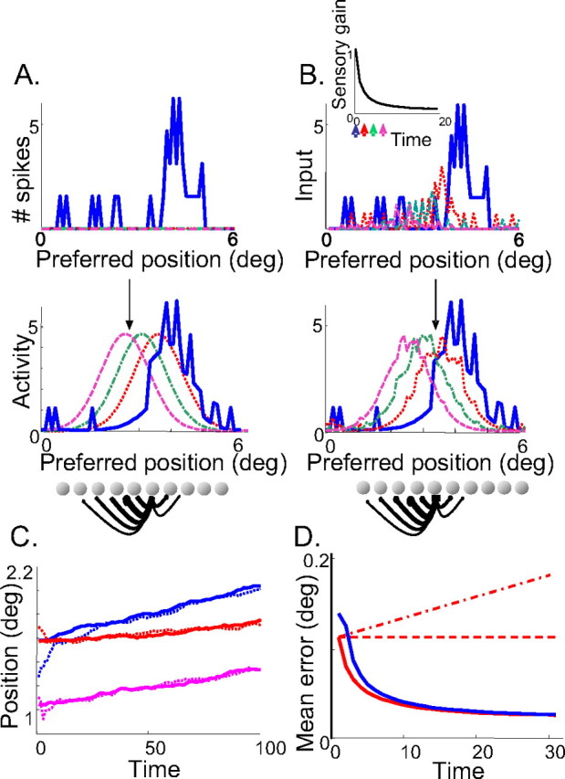
Figure 5.

Recurrent basis function network estimating arm position on-line: results. A, Distribution of activity within the three-dimensional layer, projected on the two-dimensional position/velocity map (activities of all of the cells with the same position/velocity selectivity but different force preferences are summed and collapsed on a single pixel). The panels from top to bottom represent the first, second, fourth, and sixth iterations, respectively, starting from no initial knowledge of the arm state (null activity at t = 0). The strength of activity is color-coded from red (maximum) to blue (minimum) with iso-activity contours. The position of the moving hill gives the network estimate for position and velocity. B, Estimated variance as a function of time when starting with a perfect knowledge of the arm state. Dashed/double-dotted line, Kalman filter; solid line, network estimate; dotted line, network estimate with constant sensory gains; dashed–dotted line, internal model estimate; dashed line, feedback estimate. C, Estimate variance as a function of time when starting with no initial knowledge of the arm state. The same legend as in B.
To test the network, we computed the bias and variance of the position and velocity estimates measured on many repetitions of the same task. A task corresponds to an initial arm state together with a particular sequence of force c(t) applied on the arm. If the arm dynamical equations were perfectly deterministic, repetitions of the same task would yield identical trajectories. However, because of the motor noise, each movement (each instantiation of the same task) results in a different arm trajectory. Without sensory feedback, the network would not be able to track the state of the arm properly, because it would not be able to take these random fluctuations into account. However, thanks to the noisy population codes encoding arm position and speed at each time step, the network can correct its internal estimate on-line.
We found that the network estimates were unbiased. In particular, it can predict exactly the average trajectory of the arm in response to an arbitrary succession of motor commands c(t). We compared the variance of the network estimate with the corresponding variance of an optimal Kalman filter and found that they were closely matched (the SD of the network estimate is <10% worse than the optimal variance). In Figure 5, B and C, we plotted the SD (mean error) of the Kalman filter estimates, feedback estimates (based on sensory feedback alone), internal model estimates (based on an internal prediction from the initial state without sensory feedback), and the network estimates. In Figure 5B, we started with a perfect knowledge of the arm state, i.e., we initialized the network with a noiseless Gaussian pattern of activity at position xp(0) and speed xs(0). In this condition, the network estimate, the internal model estimate, and the Kalman filter estimate start with a variance equal to zero. During the movement, all variances increase over time because of the accumulation of unpredictable motor errors (Fig. 5B). However, although the internal estimate keeps getting worse because of the accumulation of prediction errors over time, the others take advantage of the sensory feedback to correct those prediction errors, allowing the variance to converge to a finite asymptotic value.
In Figure 5C, we simulated a condition in which we assumed that the starting position is not known, which we implemented by initializing all unit activities to 0 at time 0. As a result, the Kalman filter had to build its estimate over time by integrating the somatosensory input. As can be seen in Figure 5C, the variance of the Kalman filter estimate is initially high but decreases over time as more somatosensory inputs get integrated. The network estimate follows a similar temporal profile, and after few iterations, the performance of the network is within 10% of the Kalman filter performance. Note that, in both cases, the variances of the network and the Kalman filter converge to a constant level. This constant level depends on the covariance of the motor noise and sensory noise but not on the initial knowledge about the arm state. The internal model fails entirely on this task; without knowledge of the starting position, the internal model cannot predict future positions (the performance is not plotted because the variance of the internal model estimate is infinite at all times).
To obtain the result we have described so far, we had to adjust the time-varying sensory gains λp(t) and λs(t). These gains depend on the Kalman gains and thus on the initial information present about the arm state. Thus, they have different temporal profiles depending on the initial state of knowledge, as plotted in Figure 4C. When the state of the arm is known initially, the sensory input is at first less reliable than the internal model, and the gains are small. In contrast, when no initial information is provided, the sensory input is at first more reliable, and the gains are high. However, regardless of the initial information, the gains converge to a stable regimen, like the variance.
The fact that we have to adjust the sensory gains by hand to obtain optimal performance might appear to be a strong limitation of our approach. Interestingly, however, we found that adjusting the gain over time is not quite as critical as it may seem. Thus, performance remains close to optimal when we set the gains to their value in the stable regimen without modulating them during the trajectory (Fig. 5A,B, dotted line). The main cost is in the early part of the trajectory; however, in both simulations, the variance follows the same overall temporal evolution as the variance of the Kalman filter, and it reaches the same asymptotic values. Using asymptotic values for the Kalman gains will be efficient as long as the duration of the transient (set by the level of sensory and motor noise) is relatively short compared with the duration of the movement, and as long as the statistics of the motor noise and sensory feedback is similar across a wide range of arm velocities and positions. Alternatively, varying Kalman gains could be approximated by sensory adaptation processes (see Discussion).
Experimental predictions
Our model makes two predictions. The first prediction concerns the accuracy with which human subjects can locate their hand in space while their arm is moving. If human subjects use a neural equivalent of a Kalman filter, their behavior should mirror the time evolution of the variance shown in Figure 5, B and C.
Such experiments have been performed with human subjects, in particular the experiment we have simulated in Figure 5B. This experiment involved asking subjects to locate their hand while moving their arm behind an occluder. Subjects were allowed to see the position of their hand at the beginning of the trial and, as a result, started each trial with a high accuracy estimate (i.e., a low variance). Once the movement was initiated, the visual feedback was interrupted, and subjects only received proprioceptive feedback. Wolpert et al. (1995b) reported the accuracy with which subjects located their hand as a function of the time elapsed since the onset of movement. They found that the variance of the estimate starts at a small value, begins to rise in the early part of the trial, and then reaches a plateau. This is precisely the result we report in Figure 5B. Note that our model makes a similar prediction whether we keep the sensory gains constant or adjust them on-line. Therefore, this experiment suggests that humans use an internal model, but it does not tell us whether humans adjust their sensory gains on-line.
Another recent study suggests that the human brain uses a Kalman filter for on-line control of reaching arm movement (Saunders and Knill, 2005). In particular, humans are able to weight two sensory cues differentially (arm movement direction and distance in their case) according to their relative reliability for the task. This is also true in our model: position input is more reliable than velocity input (or, more exactly, the internal estimate of velocity is much more precise and relies less on sensory feedback than the internal estimate of position). Position input is more informative for determining the arm state and is thus weighted more strongly.
The second experimental prediction has to do with the response property of single neurons in the motor system. As can be seen in Figure 5A, the shape of the hill of activity in the basis function layer is not perfectly circular; it is elongated and tilted. This translates into a surprising prediction for the tuning curves to position and velocity. If we plot the tuning curve of a unit to arm velocity, we find that the gain of the tuning curves (i.e., their amplitude) is modulated by the position of the arm. Furthermore, the preferred velocity shifts to faster motion for arm position that are situated farther in the direction of the movement (Fig. 6A). Vice versa, if we plot the tuning curve of the same cell to arm position for different arm velocity, we find that the tuning curve to position is gain modulated by velocity and shifted in the direction of the movement for higher velocities.
Figure 6.

Experimental predictions from a recurrent basis function network estimating arm position on-line. A, Tuning curves of a sensorimotor unit to velocity for two different positions of the arm. B, Preferred direction of a sensorimotor unit as a function of arm position. Circles represent the arm position in 2D. Lines point away from the circles in the direction of the arm velocity vector for which the unit is maximally active when the arm is at that particular position. The length of the line is proportional to the response of the unit when the arm moves at its preferred velocity. The global preferences of this unit are for xi(t) = (15 cm, 15 cm) and yi(t) = (0 cm.s−1, 0 cm.s−1). However, the preferred velocity vector measured at a particular arm position rotates with the arm. The inset on the top right of the figure represents the response of this unit as a function of arm movement direction (arm moving at 150 cm.s−1) when the arm is at position x(t) = (15 cm, 15 cm) (solid line) together with the best-fitting cosine tuning curve (dashed line). C, Same as in B but for a unit preferring xi(t) = (0 cm, 0 cm), yi(t) = (150 cm.s−1, 150 cm.s−1). D, Direction of the population vector for a constant arm velocity yi(t) = (150 cm.s−1, 150 cm.s−1) for all positions of the arm. E, Same as in A but with the motor noise increased by a factor of 10. The somatosensory input is now more reliable than the internal model, and the tuning curve no longer shifts with arm position. F, Same as in E but with the motor noise increased by a factor of 10. The preferred direction no longer rotates with arm position.
To explore these predictions in 2D, we constructed a network in which the intermediate layer represents six variables instead of three: two variables for spatial position xp, yp, two for velocity xs, ys and two for end-point force xc, yc (see Materials and Methods). The dynamics of the arm in the horizontal (x) and vertical (y) dimensions are assumed to be the same. Thus, in addition to Equation 18 describing the dynamics of x(t) = (xp(t),xs(t)), the network implements the following dynamical equation for y(t) = (yp(t),ys(t)):
c′(t) = (0,c(t)) is a motor command at time t corresponding to the end-point muscular force along the y-axis, and ε′(t) is a motor noise term.
We measured the velocity tuning curves of the sensorimotor units of a network tracking the arm in 2D for different positions of the arm (same as Fig. 6A, but in 2D). In 2D, the orientation of the velocity vector, v⃗=(xs, ys), defines the movement direction. We found that the sensorimotor units are broadly tuned to movement direction, with tuning curves approximately cosine shaped (Fig. 6B). These tuning curves are modulated in height (or gain) by arm speed. This modulation is bell shaped but extremely broad. As a result, for a large majority of the units, the gain modulation by speed is monotonic and almost linear in the natural range of arm velocity (Fig. 6C, inset). Note that, as shown in supplemental material (available at www.jneurosci.org), the performance of the network does not depend on the exact shape of the tuning curves to speed and position, as long as these curves form a basis set (i.e., sigmoids, sines, cosines, rectified linear curves, and Gaussians are basis functions) and are similar to the tuning of the sensory feedback (these constraints are detailed in the mathematical proof in supplemental material, available at www.jneurosci.org).
The direction tuning curves also change with arm position. However, in contrast to arm speed, which only affects the gain of the tuning curves, arm position changes both the gain and the preferred direction of the cell. This result is illustrated in Figure 6, B and C, which shows the preferred direction of two different units as a function of arm positions. The length of the lines in Figure 6 indicates the response strength of the unit when the arm moves in its preferred direction at this location in space. As can be seen on the figure, the direction and length of the lines change with arm position, indicating a change in the preferred direction and the gain of the neuron as a function of arm position.
These results are consistent with what we know of the velocity tuning of neurons in the motor and premotor cortices. Thus, their direction tuning curves are approximately cosine-tuned to movement direction (Georgopoulos et al., 1982), and neural responses are gain modulated by arm posture and arm speed in these areas (Boussaoud, 1995; Caminiti et al., 1999; Kakei et al., 2003; Paninski et al., 2004). This gain modulation is usually reported to be monotonically increasing with arm speed, either using the indirect evidence that the length of the population vector increases linearly with speed (Ashe et al., 1993; Moran and Schwartz, 1999) or by measuring position and velocity tuning curves through spike reverse correlation techniques during tracking movements (Paninski et al., 2004). In contrast, we used nonmonotonic (bell-shaped) velocity tuning curves in our model, just like we did for position. However, as mentioned above, our Gaussian tuning curves are so broad that most of them appear to be monotonic over the range of natural arm speeds Moreover, as shown in the supplemental material (available at www.jneurosci.org), our conclusions are not restricted to Gaussian tuning curves but hold for other types of tuning curves such as sigmoidal or rectified linear functions.
Another result that is consistent with experimental observation is the rotation of preferred directions with arm position, which has been reported in motor and premotor cortices (Caminiti et al., 1990, 1991). In the motor and premotor cortices, the rotation of preferred direction with arm position has two important properties: (1) the preferred direction vector averaged across all neurons rotates in the same direction as the arm, and (2) despite these rotations of the preferred directions of individual cells, the population vector (Georgopoulos et al., 1982) points in the direction of the movement. Our model reproduces both of these effects, as shown in Figure 6B–D. The preferred direction of the individual cell rotates in the direction of arm displacement (Fig. 6B,C), whereas the population vector points in the real direction of the movement (Fig. 6D).
The reason for the rotation of preferred directions can be understood intuitively. The prediction of a future arm state introduces correlations between position and velocity. For example, the future arm position is a function of the previous arm position and velocity. These correlations are reflected by correlations in the population representation of the two variables. The tilt in the population activity pattern (and thus the noninvariance of velocity coding to position, and vice versa) is caused by the predictive lateral connections within the sensorimotor layer. However, this recurrent prediction is combined on-line with the sensory input, which is independent for position and velocity. The resulting neural activation is a trade-off between the correlated predictive representation and the uncorrelated sensory input. If the sensory input is much more reliable than the internal prediction, the noninvariance and tuning curve shifts disappear. The sensorimotor cell appears to be tuned to velocity and gain modulated by position, or vice versa (Fig. 6E). Similarly, the sensorimotor cell appears to have a constant (not rotating) velocity vector in 2D (Fig. 6F). In other words, the extent to which the tuning curves are shifted and gain modulated depends on the respective reliability of the internal estimate and the sensory feedback. To our knowledge, this prediction has never been tested.
The fact that the population vector continues to point in the direction of the movement despite rotation of individual preferred directions can also be easily explained. This is a consequence of the fact that the network estimates are unbiased: the pattern of activity on the layer peaks on average at the true position and velocity of the arm. As a consequence, the population vector (as well as the center-of-mass estimator or any other unbiased estimator used to read the velocity encoded by the population of units) will point in the direction of the movement, even if the preferred direction of each individual unit rotates with the arm.
Although our model captures all of the essential features of the data reported in premotor and motor cortex, it does not account for one result, namely the fact that the rotation in preferred direction with arm position is different in each neuron. This result, however, would be easy to implement. In the simulation presented here, we have assumed from the sake of simplicity that all units gave the same relative confidence to the sensory input and the input coming from lateral connections. However, in biological systems, the reliability of the sensory input is likely to vary widely in different cells or different cell types, leading to a strong variability in the extent of the preferred direction rotation.
Our model is not the first one to account for these experimental observations in premotor and motor cortices. As shown by Zhang and Sejnowski (1999), cosine direction tuning curves and gain modulation by speed are to be expected from sensory or motor cells responding to motion in two-dimensional or three-dimensional space, regardless of the mechanism involved. The main contribution of our model is to provide quantitative predictions for the shifts in the preferred direction of each neuron with arm position. Several alternative explanations have been offered to explain the rotation, including the use of a joint-related coordinate system by motor cells (Tanaka, 1994), spatially uniform coding in kinetic coordinates (Ajemian et al., 2001), the fact that motor cells control groups of muscles that are themselves tuned to movement direction (Turner et al., 1995), or the consequence of a visuomotor coordinate transform (Burnod et al., 1992; Salinas and Abbot, 1995). In our model, this noninvariance of the representation arises naturally from principles of optimal sensorimotor integration.
Mathematical proof
As shown in the supplemental material (available at www.jneurosci.org), the two examples we have presented are instances of a general theory of optimal sensorimotor integration by iterative basis function (IBF) networks. These models work by projecting neural activity toward a manifold of noiseless population codes. On this manifold, activities are updated over time to reflect the predictable temporal evolution for the sensory and motor state (see Materials and Methods). Near optimality is guaranteed as long as the following conditions are met: (1) the sensorimotor dynamical equations are locally linear. (2) The motor noise is Gaussian, independent for the different state variables, and white. (3) Sensory gains are adjusted to the relative reliability of the sensory input compared with the internal model.
Discussion
We have shown that IBF networks can integrate optimally time-varying sensory inputs and efferent motor commands, effectively implementing Kalman filters with population codes.
Adjusting the sensory and internal model contributions
One of the important features of a Kalman filter is the Kalman gain, that is, the gain of the sensory input compared with the internal model. This gain must be modified over time to achieve optimal temporal integration. In our model, this gain was implemented by adjusting the synaptic weights of the sensory afferences according to the ratio of the noise in the sensory feedback and the uncertainty in the internal estimate. Such rapid changes of synaptic efficacy can take place in the cortex through either short-term synaptic potentiation and depression (Thomson and Deuchars, 1994) or spike-timing-dependent plasticity (Markram et al., 1997), but it is presently unclear whether these changes are sufficient to trigger the synaptic changes required by a Kalman filter. For static variables, Wu et al. (2003) have already shown that Hebbian learning is sufficient to adjust the gain of a neural Kalman filter. For time-varying variables, as we have considered in this study, the problem is significantly more difficult and would deserve to be explored in future studies.
The temporal evolution of the Kalman gains could also be implemented by response adaptation within primary sensory areas, which leads to a gradual decay of neural activity during prolonged presentation of sensory stimuli. Interestingly, it was recently suggested that this gradual decay follows a power law (scale invariant) of the form St = So/(t + l)n (P. J. Drew and L. F. Abbott, unpublished observations). This is an important observation because the temporal evolution of Kalman gains is also, in many cases, close to a power law. For example, in cases involving a single sensory variable (as in our object tracking example), the sensory gain computed from Kalman equations initially evolves according to λt = 1/(t + 1) before converging to a constant level.
Ultimately, however, it is possible that the nervous system does not adjust its Kalman gain optimally. As we have seen, keeping the gain constant can actually lead to near-optimal behaviors in many situations (Fig. 5B,C).
Motor control, sensory delays, and inverse models
Although we have applied our approach to sensory problems, IBF networks could be readily adapted to deal with optimal motor control. Motor control involves the same set of tools we have been using thus far (internal models and appropriate weighting of the sensory feedback) and, indeed, Kalman filters are commonly used to model on-line control of reaching movements by visual/proprioceptive feedback (Desmurget and Grafton, 2000; Wolpert and Ghahramani, 2000; Saunders and Knill, 2005). The main difference between optimal sensorimotor integration, as we have considered in this study, and optimal motor control is the temporal discrepancy between the arrival of the sensory feedback and the on-line correction of movement. The sensory input is necessarily delayed by a few tens or hundreds of milliseconds, whereas on-line correction of movement trajectories needs to occur in real time, based on the current (nondelayed) motor state.
In our models, the current position and velocity of the arm can be estimated by feeding the activities from the sensorimotor layer into a similar network performing internal prediction but not receiving any sensory input. Similarly, IBF networks receiving sensory inputs with longer delays could predict the activity of IBF networks with shorter delays (e.g., knowing what the arm state was 100 ms ago, from the delayed visual feedback, one can predict were it will be 50 ms later, when the proprioceptive feedback arrives), effectively integrating all sensory inputs together (Fig. 7A, solid arrows).
Figure 7.

Generalization of the model. A, Sensory inputs with different delays could be implemented by two networks encoding the best state estimate for this delay and interconnected. Connections from longer delays (plain arrows) implement a internal model. Connections from shorter to longer delays (dashed arrows) implement an inverse model. This inverse model can also compute the most appropriate motor commands given the current estimated state x̂(t) and a future “desired” state x̂(t + d). B, Combinatorial explosion and modularity. An internal model for the arm dynamics can be implemented by a bimodular network predicting velocity from velocity and force and position from position and velocity. C, Result of the bimodular network (same legend as in Fig. 5B).
Note that it is also possible to predict the past state from the current state (e.g., where was my arm in space 100 ms ago, knowing that it is there now?) and to compute what motor command would bring the arm to a desired future state (e.g., knowing where my arm is now, and where I want it to be 800 ms later, what motor command should I use?). Connections going in the other direction (from sensorimotor maps to motor areas) could compute the optimal motor command to reach a desired sensory state (Fig. 7A, dashed arrows), providing a neural basis for motor learning (Jordan and Rumelhart, 1992) and optimal motor control (Scott and Norman, 2003; Todorov, 2004).
This extended model predicts the existence of sensorimotor cells tuned to position and velocity at various temporal delays compared with the current arm state. Interestingly, recent data suggest the existence of such a representation in M1 (Paninski et al., 2004).
Noninvariant tuning properties arising from optimality principles in sensorimotor areas
More generally, our model also has important implications for neural representations in sensorimotor areas. We predict in particular that neurons implementing optimal sensorimotor filters should exhibit predictive activity, generated by the internal model, in addition to the usual sensory and motor responses. The “visual remapping” activity reported in lateral intraparietal area (LIP) is the best known example of such predictive signals: before a saccade, some neurons in LIP respond to a visual target that will appear in their receptive field after the saccade (Duhamel et al., 1992). We expect that similar results will be found in sensorimotor areas, in particular the ones controlling the arms. For example, sensorimotor neurons should respond during or immediately before an arm movement in anticipation of visual, tactile, or proprioceptive feedback occurring at a later time along the arm trajectory.
Another important prediction concerns the invariance, or rather the lack of invariance, of the tuning curves. It is common in neurophysiological experiments to seek the frame of reference in which a receptive field is invariant. In IBF networks, it is simply impossible to identify any frame of reference in which the tuning curves to velocity, position, or force are invariant because those variables interact with one another. For instance, as illustrated in Figure 6A, the position of the tuning curve to arm velocity depends on the position of the arm. Moreover, this dependency changes with the level of noise corrupting the proprioceptive feedback (Fig. 6C), and more generally on the Kalman gains. As a result, the tuning curve to velocity of a unit can change over the course of a single movement, because the Kalman gains themselves change. This strong dependence on the context and the task implies that tuning curves in the motor cortex are unlikely to stay invariant across movements and time.
This lack of invariance has been reported in M1 and premotor cortex, and has led to a fierce debate as to whether M1 neurons encode cinematic versus dynamic coordinates and extrinsic versus intrinsic coordinates (Georgopoulos and Ashe, 2000; Moran and Schwartz, 2000; Scott, 2000; Todorov, 2000). We are suggesting that the lack of invariance may in part be caused by the use of recurrent basis function maps involved in optimal sensorimotor transformations.
Combinatorial explosion and modularity
Basis function maps can implement a very large set of nonlinear transformations (Poggio, 1990; Girosi et al., 1995; Pouget and Sejnowski, 1997). However, there is a price to pay in terms of number of units and connections needed: this number grows exponentially with the number of dimensions or variables represented.
One solution to this problem is modularity. Instead of one central map, we can use several interconnected modules representing subsets of the variables. For example, if we use one map to represent the position, velocity, and force of the arm, we need in the order of 103 neurons and 106 connections. Instead, we can use two maps, one for position and velocity and another one for velocity and force. Each map requires 102 neurons for a total of 2 102 neurons, instead of 103. Moreover, the number of connections is now of the order of 104 instead of 106. To connect the two modules, we can use the velocity/force module to predict the velocity at the next time step, and we can send this signal to the velocity/position module whose output is the prediction of the position at the next time step given the previous position and the predicted velocity (Fig. 7B).
This modular architecture requires substantially less units and connections, but there is cost in terms of performance. The modular network cannot represent the correlations between position and velocity: in particular, somatosensory feedback about position cannot be used to correct the estimate of velocity, and vice versa. As shown in Figure 7C, this results in suboptimal performance. For systems with a large number of degrees of freedom, as is the case for the human arms, such compromise between accuracy and computational cost is difficult to avoid.
Note that the trade-off between the number of neurons and the accuracy is not as severe as it might seem at first. The accuracy of the model can still be high with a very small number of neurons per dimension. In particular, the SD of the network position estimate is several orders of magnitude smaller than the spacing between two successive preferred positions in the layer. In fact, this accuracy depends on the total number of neurons in the layer receiving uncorrelated sensory inputs tuned to position, not the number of neurons per dimension. Finally, taking into account the correlations between two variables contributes significantly to the accuracy only when they are strongly correlated (i.e., position and velocity). For more weakly correlated variables, the loss in accuracy resulting from separating them into two modules will often be negligible.
Toward a neural theory of Bayesian inference
Our model provides a significant step toward understanding how neural circuits implement optimal sensorimotor filters, and in particular Kalman filters, but it remains limited to Gaussian distributions. To extend this work to the general case, we first need to understand how to encode arbitrary probability distributions with population codes. Several coding schemes have been explored previously (Zemel et al., 1998; Weiss and Fleet, 2002; Barber et al., 2003; Mazurek et al., 2003; Sahani and Dayan, 2003; Ma et al., 2006), and several groups are exploring how to use these schemes for optimal filtering (Deneve, 2004; Rao, 2004). Whether any of these schemes is consistent with the response of cortical neurons remains to be determined, but this topic should be the target of intense research in the next few years.
Footnotes
A.P. was supported by National Institute on Drug Abuse Grant RO1 DA022780-01 and a grant from the James S. McDonnell Foundation. J.-R.D. and A.P. were supported by National Science Foundation Grants BCS0346785 and BCS0446730. S.D. was supported by the European Grant BACS FP6-IST-027140.
References
- Abbott and Blum, 1996.Abbott LF, Blum KI. Functional significance of long-term potentiation for sequence learning and prediction. Cereb Cortex. 1996;6:406–416. doi: 10.1093/cercor/6.3.406. [DOI] [PubMed] [Google Scholar]
- Ajemian et al., 2001.Ajemian R, Bullock D, Grossberg S. A model of movement coordinates in the motor cortex: posture-dependent changes in the gain and direction of single cell tuning curves. Cereb Cortex. 2001;11:1124–1135. doi: 10.1093/cercor/11.12.1124. [DOI] [PubMed] [Google Scholar]
- Anderson and Moore, 1979.Anderson B, Moore J. Optimal filtering. Englewood Cliffs, NJ: Prentice Hall; 1979. [Google Scholar]
- Ashe et al., 1993.Ashe J, Taira M, Smyrnis N, Pellizzer G, Georgakopoulos T, Lurito JT, Georgopoulos AP. Motor cortical activity preceding a memorized movement trajectory with an orthogonal bend. Exp Brain Res. 1993;95:118–130. doi: 10.1007/BF00229661. [DOI] [PubMed] [Google Scholar]
- Ballard et al., 2000.Ballard DH, Hayhoe MM, Salgian G, Shinoda H. Spatio-temporal organization of behavior. Spat Vis. 2000;13:321–333. doi: 10.1163/156856800741144. [DOI] [PubMed] [Google Scholar]
- Barber et al., 2003.Barber MJ, Clark JW, Anderson CH. Neural representation of probabilistic information. Neural Comput. 2003;15:1843–1864. doi: 10.1162/08997660360675062. [DOI] [PubMed] [Google Scholar]
- Boussaoud, 1995.Boussaoud D. Primate premotor cortex: modulation of preparatory neuronal activity by gaze angle. J Neurophysiol. 1995;73:886–889. doi: 10.1152/jn.1995.73.2.886. [DOI] [PubMed] [Google Scholar]
- Brunel and Nadal, 1998.Brunel N, Nadal JP. Mutual information, Fisher information, and population coding. Neural Comput. 1998;10:1731–1757. doi: 10.1162/089976698300017115. [DOI] [PubMed] [Google Scholar]
- Burnod et al., 1992.Burnod Y, Grandguillaume P, Otto I, Ferraina S, Johnson PB, Caminiti R. Visuomotor transformations underlying arm movements toward visual targets: a neural network model of cerebral cortical operations. J Neurosci. 1992;12:1435–1453. doi: 10.1523/JNEUROSCI.12-04-01435.1992. [DOI] [PMC free article] [PubMed] [Google Scholar]
- Caminiti et al., 1990.Caminiti R, Johnson PB, Urbano A. Making arm movements within different parts of space: dynamic aspects in the primate motor cortex. J Neurosci. 1990;10:2039–2058. doi: 10.1523/JNEUROSCI.10-07-02039.1990. [DOI] [PMC free article] [PubMed] [Google Scholar]
- Caminiti et al., 1991.Caminiti R, Johnson PB, Galli C, Ferraina S, Burnod Y. Making arm movements within different parts of space: the premotor and motor cortical representation of a coordinate system for reaching to visual targets. J Neurosci. 1991;11:1182–1197. doi: 10.1523/JNEUROSCI.11-05-01182.1991. [DOI] [PMC free article] [PubMed] [Google Scholar]
- Caminiti et al., 1999.Caminiti R, Genovesio A, Marconi B, Mayer A, Onorati P, Ferraina S, Mitsuda T, Giannetti S, Squatrito S, Maioli M, Molinari M. Early coding of reaching: frontal and parietal association connections of parieto-occipital cortex. Eur J Neurosci. 1999;11:3339–3345. doi: 10.1046/j.1460-9568.1999.00801.x. [DOI] [PubMed] [Google Scholar]
- Dayan and Balleine, 2002.Dayan P, Balleine BW. Reward, motivation, and reinforcement learning. Neuron. 2002;36:285–298. doi: 10.1016/s0896-6273(02)00963-7. [DOI] [PubMed] [Google Scholar]
- Deneve, 2004.Deneve S. Bayesian inference with recurrent spiking networks. In: Lawrence KS, Weiss Y, Bottou L, editors. Advances in neural information processing system. Cambridge: MIT; 2004. pp. 353–360. [Google Scholar]
- Deneve et al., 1999.Deneve S, Latham P, Pouget A. Reading population codes: a neural implementation of ideal observers. Nat Neurosci. 1999;2:740–745. doi: 10.1038/11205. [DOI] [PubMed] [Google Scholar]
- Deneve et al., 2001.Deneve S, Latham P, Pouget A. Efficient computation and cue integration with noisy population codes. Nat Neurosci. 2001;4:826–831. doi: 10.1038/90541. [DOI] [PubMed] [Google Scholar]
- Desmurget and Grafton, 2000.Desmurget M, Grafton S. Forward modeling allows feedback control for fast reaching movements. Trends Cogn Sci. 2000;4:423–431. doi: 10.1016/s1364-6613(00)01537-0. [DOI] [PubMed] [Google Scholar]
- Dorris and Glimcher, 2004.Dorris MC, Glimcher PW. Activity in posterior parietal cortex is correlated with the relative subjective desirability of action. Neuron. 2004;44:365–378. doi: 10.1016/j.neuron.2004.09.009. [DOI] [PubMed] [Google Scholar]
- Duhamel et al., 1992.Duhamel JR, Colby CL, Goldberg ME. The updating of the representation of visual space in parietal cortex by intended eye movements. Science. 1992;255:90–92. doi: 10.1126/science.1553535. [DOI] [PubMed] [Google Scholar]
- Fu et al., 2004.Fu YX, Shen Y, Gao H, Dan Y. Asymmetry in visual cortical circuits underlying motion-induced perceptual mislocalization. J Neurosci. 2004;24:2165–2171. doi: 10.1523/JNEUROSCI.5145-03.2004. [DOI] [PMC free article] [PubMed] [Google Scholar]
- Georgopoulos and Ashe, 2000.Georgopoulos AP, Ashe J. One motor cortex, two different views. Nat Neurosci. 2000;3:963. doi: 10.1038/79882. author reply 964–965. [DOI] [PubMed] [Google Scholar]
- Georgopoulos et al., 1982.Georgopoulos AP, Kalaska JF, Caminiti R, Massey JT. On the relations between the direction of two-dimensional arm movements and cell discharge in primate motor cortex. J Neurosci. 1982;2:1527–1537. doi: 10.1523/JNEUROSCI.02-11-01527.1982. [DOI] [PMC free article] [PubMed] [Google Scholar]
- Girosi et al., 1995.Girosi F, Jones M, Poggio T. Regularization theory and neural network architectures. Neural Comput. 1995;7:219–269. [Google Scholar]
- Gold and Shadlen, 2003.Gold JI, Shadlen MN. The influence of behavioral context on the representation of a perceptual decision in developing oculomotor commands. J Neurosci. 2003;23:632–651. doi: 10.1523/JNEUROSCI.23-02-00632.2003. [DOI] [PMC free article] [PubMed] [Google Scholar]
- Heeger, 1992a.Heeger DJ. Normalization of cell responses in cat striate cortex. Vis Neurosci. 1992a;9:181–197. doi: 10.1017/s0952523800009640. [DOI] [PubMed] [Google Scholar]
- Heeger, 1992b.Heeger DJ. Half-squaring in responses of cat striate cells. Vis Neurosci. 1992b;9:427–443. doi: 10.1017/s095252380001124x. [DOI] [PubMed] [Google Scholar]
- Jones et al., 2002.Jones KE, Hamilton AF, Wolpert DM. Sources of signal-dependent noise during isometric force production. J Neurophysiol. 2002;88:1533–1544. doi: 10.1152/jn.2002.88.3.1533. [DOI] [PubMed] [Google Scholar]
- Jordan and Rumelhart, 1992.Jordan MI, Rumelhart DE. Forward models: supervised learning with a distal teacher. Cogn Sci. 1992;16:307–354. [Google Scholar]
- Kakei et al., 2003.Kakei S, Hoffman DS, Strick PL. Sensorimotor transformations in cortical motor areas. Neurosci Res. 2003;46:1–10. doi: 10.1016/s0168-0102(03)00031-2. [DOI] [PubMed] [Google Scholar]
- Kawato, 1999.Kawato M. Internal models for motor control and trajectory planning. Curr Opin Neurobiol. 1999;9:718–727. doi: 10.1016/s0959-4388(99)00028-8. [DOI] [PubMed] [Google Scholar]
- Latham et al., 2003.Latham PE, Deneve S, Pouget A. Optimal computation with attractor networks. J Physiol Paris. 2003;97:683–694. doi: 10.1016/j.jphysparis.2004.01.022. [DOI] [PubMed] [Google Scholar]
- Lee et al., 1988.Lee C, Rohrer WH, Sparks DL. Population coding of saccadic eye movements by neurons in the superior colliculus. Nature. 1988;332:357–360. doi: 10.1038/332357a0. [DOI] [PubMed] [Google Scholar]
- Lee et al., 1998.Lee D, Port NL, Kruse W, Georgopoulos AP. Variability and correlated noise in the discharge of neurons in motor and parietal areas of the primate cortex. J Neurosci. 1998;18:1161–1170. doi: 10.1523/JNEUROSCI.18-03-01161.1998. [DOI] [PMC free article] [PubMed] [Google Scholar]
- Ma et al., 2006.Ma WJ, Beck JM, Latham PE, Pouget A. Bayesian inference with probabilistic population codes. Nat Neurosci. 2006;9:1432–1438. doi: 10.1038/nn1790. [DOI] [PubMed] [Google Scholar]
- Markram et al., 1997.Markram H, Lubke J, Frotscher M, Sakmann B. Regulation of synaptic efficacy by coincidence of postsynaptic APs and EPSPs. Science. 1997;275:213–215. doi: 10.1126/science.275.5297.213. [DOI] [PubMed] [Google Scholar]
- Mazurek et al., 2003.Mazurek ME, Roitman JD, Ditterich J, Shadlen MN. A role for neural integrators in perceptual decision making. Cereb Cortex. 2003;13:1257–1269. doi: 10.1093/cercor/bhg097. [DOI] [PubMed] [Google Scholar]
- Mehta and Schaal, 2002.Mehta B, Schaal S. Forward models in visuomotor control. J Neurophysiol. 2002;88:942–953. doi: 10.1152/jn.2002.88.2.942. [DOI] [PubMed] [Google Scholar]
- Moran and Schwartz, 1999.Moran DW, Schwartz AB. Motor cortical representation of speed and direction during reaching. J Neurophysiol. 1999;82:2676–2692. doi: 10.1152/jn.1999.82.5.2676. [DOI] [PubMed] [Google Scholar]
- Moran and Schwartz, 2000.Moran DW, Schwartz AB. One motor cortex, two different views. Nat Neurosci. 2000;3:963. doi: 10.1038/79880. author reply 963–965. [DOI] [PubMed] [Google Scholar]
- Paninski et al., 2004.Paninski L, Fellows MR, Hatsopoulos NG, Donoghue JP. Spatiotemporal tuning of motor cortical neurons for hand position and velocity. J Neurophysiol. 2004;91:515–532. doi: 10.1152/jn.00587.2002. [DOI] [PubMed] [Google Scholar]
- Papoulis, 1991.Papoulis A. Columbus, OH: McGraw-Hill; 1991. Probability, random variables, and stochastic process. [Google Scholar]
- Poggio, 1990.Poggio T. A theory of how the brain might work. Cold Spring Harb Symp Quant Biol. 1990;55:899–910. doi: 10.1101/sqb.1990.055.01.084. [DOI] [PubMed] [Google Scholar]
- Pouget and Sejnowski, 1997.Pouget A, Sejnowski T. Spatial transformations in the parietal cortex using basis functions. J Cogn Neurosci. 1997;9:222–237. doi: 10.1162/jocn.1997.9.2.222. [DOI] [PubMed] [Google Scholar]
- Pouget et al., 1998.Pouget A, Zhang K, Deneve S, Latham PE. Statistically efficient estimation using population code. Neural Comput. 1998;10:373–401. doi: 10.1162/089976698300017809. [DOI] [PubMed] [Google Scholar]
- Pouget et al., 2002.Pouget A, Deneve S, Duhamel JR. A computational perspective on the neural basis of multisensory spatial representations. Nat Rev Neurosci. 2002;3:741–747. doi: 10.1038/nrn914. [DOI] [PubMed] [Google Scholar]
- Rao, 2004.Rao RP. Bayesian computation in recurrent neural circuits. Neural Comput. 2004;16:1–38. doi: 10.1162/08997660460733976. [DOI] [PubMed] [Google Scholar]
- Riehle et al., 1997.Riehle A, Grun S, Diesmann M, Aertsen A. Spike synchronization and rate modulation differentially involved in motor cortical function. Science. 1997;278:1950–1953. doi: 10.1126/science.278.5345.1950. [DOI] [PubMed] [Google Scholar]
- Sahani and Dayan, 2003.Sahani M, Dayan P. Doubly distributional population codes: simultaneous representation of uncertainty and multiplicity. Neural Comput. 2003;15:2255–2279. doi: 10.1162/089976603322362356. [DOI] [PubMed] [Google Scholar]
- Salinas and Abbot, 1995.Salinas E, Abbot LF. Transfer of coded information from sensory to motor networks. J Comput Neurosci. 1995;1:89–107. doi: 10.1523/JNEUROSCI.15-10-06461.1995. [DOI] [PMC free article] [PubMed] [Google Scholar]
- Saunders and Knill, 2005.Saunders JA, Knill DC. Humans use continuous visual feedback from the hand to control both the direction and distance of pointing movements. Exp Brain Res. 2005;162:458–473. doi: 10.1007/s00221-004-2064-1. [DOI] [PubMed] [Google Scholar]
- Schmidt et al., 1979.Schmidt RA, Zelaznik H, Hawkins B, Frank JS, Quinn JT., Jr Motor-output variability: a theory for the accuracy of rapid motor acts. Psychol Rev. 1979;47:415–451. [PubMed] [Google Scholar]
- Scott, 2000.Scott SH. Reply to “One motor cortex, two different views.”. Nat Neurosci. 2000;3:964–965. doi: 10.1038/79888. [DOI] [PubMed] [Google Scholar]
- Scott and Norman, 2003.Scott SH, Norman KE. Computational approaches to motor control and their potential role for interpreting motor dysfunction. Curr Opin Neurol. 2003;16:693–698. doi: 10.1097/01.wco.0000102631.16692.71. [DOI] [PubMed] [Google Scholar]
- Shadlen and Newsome, 1994.Shadlen MN, Newsome WT. Noise, neural codes and cortical organization. Curr Opin Neurobiol. 1994;4:569–579. doi: 10.1016/0959-4388(94)90059-0. [DOI] [PubMed] [Google Scholar]
- Slifkin and Newell, 1999.Slifkin AB, Newell KM. Noise, information transmission, and force variability. J Exp Psychol Hum Percept Perform. 1999;25:837–851. doi: 10.1037//0096-1523.25.3.837. [DOI] [PubMed] [Google Scholar]
- Sugrue et al., 2004.Sugrue LP, Corrado GS, Newsome WT. Matching behavior and the representation of value in the parietal cortex. Science. 2004;304:1782–1787. doi: 10.1126/science.1094765. [DOI] [PubMed] [Google Scholar]
- Tanaka, 1994.Tanaka S. Hypothetical joint-related coordinate systems in which populations of motor cortical neurons code direction of voluntary arm movements. Neurosci Lett. 1994;180:83–86. doi: 10.1016/0304-3940(94)90493-6. [DOI] [PubMed] [Google Scholar]
- Thomson and Deuchars, 1994.Thomson AM, Deuchars J. Temporal and spatial properties of local circuits in neocortex. Trends Neurosci. 1994;17:119–126. doi: 10.1016/0166-2236(94)90121-x. [DOI] [PubMed] [Google Scholar]
- Todorov, 2000.Todorov E. Direct cortical control of muscle activation in voluntary arm movements: a model. Nat Neurosci. 2000;3:391–398. doi: 10.1038/73964. [DOI] [PubMed] [Google Scholar]
- Todorov, 2004.Todorov E. Optimality principles in sensorimotor control. Nat Neurosci. 2004;7:907–915. doi: 10.1038/nn1309. [DOI] [PMC free article] [PubMed] [Google Scholar]
- Tolhurst et al., 1982.Tolhurst D, Movshon J, Dean A. The statistical reliability of signals in single neurons in cat and monkey visual cortex. Vision Res. 1982;23:775–785. doi: 10.1016/0042-6989(83)90200-6. [DOI] [PubMed] [Google Scholar]
- Turner et al., 1995.Turner RS, Owens JW, Jr, Anderson ME. Directional variation of spatial and temporal characteristics of limb movements made by monkeys in a two-dimensional work space. J Neurophysiol. 1995;74:684–697. doi: 10.1152/jn.1995.74.2.684. [DOI] [PubMed] [Google Scholar]
- Vogels et al., 1989.Vogels R, Spileers W, Orban GA. The response variability of striate cortical neurons in the behaving monkey. Exp Brain Res. 1989;77:432–436. doi: 10.1007/BF00275002. [DOI] [PubMed] [Google Scholar]
- Weiss and Fleet, 2002.Weiss Y, Fleet D. Velocity likelihood in biological and machine vision. In: Rao RPN, Olshausen BA, Lewicki MS, editors. Probabilistic models of the brain: perception and neural function. Boston: MIT; 2002. pp. 77–96. [Google Scholar]
- Wolpert and Ghahramani, 2000.Wolpert DM, Ghahramani Z. Computational principles of movement neuroscience. Nat Neurosci. 2000;3(Suppl):1212–1217. doi: 10.1038/81497. [DOI] [PubMed] [Google Scholar]
- Wolpert et al., 1995a.Wolpert DM, Ghahramani Z, Jordan M. An internal model for sensorimotor integration. Science. 1995a;269:1880–1882. doi: 10.1126/science.7569931. [DOI] [PubMed] [Google Scholar]
- Wolpert et al., 1995b.Wolpert DM, Ghahramani Z, Jordan MI. Forward dynamic models in human motor control: psychophysical evidence. In: Tesauro G, Touretzki DS, Lenn TK, editors. Advances in neural information processing system. Cambridge, MA: MIT; 1995b. [Google Scholar]
- Wu et al., 2003.Wu S, Chen D, Niranjan M, Amari S. Sequential Bayesian decoding with a population of neurons. Neural Comput. 2003;15:993–1012. doi: 10.1162/089976603765202631. [DOI] [PubMed] [Google Scholar]
- Zemel et al., 1998.Zemel RS, Dayan P, Pouget A. Probabilistic interpretation of population codes. Neural Comput. 1998;10:403–430. doi: 10.1162/089976698300017818. [DOI] [PubMed] [Google Scholar]
- Zhang and Sejnowski, 1999.Zhang K, Sejnowski TJ. A theory of geometric constraints on neural activity for natural three-dimensional movement. J Neurosci. 1999;19:3122–3145. doi: 10.1523/JNEUROSCI.19-08-03122.1999. [DOI] [PMC free article] [PubMed] [Google Scholar]
- Zohary, 1992.Zohary E. Population coding of visual stimuli by cortical neurons tuned to more than one dimension. Biol Cybern. 1992;66:265–272. doi: 10.1007/BF00198480. [DOI] [PubMed] [Google Scholar]