Posteromedial Parietal Cortical Activity and Inputs Predict Tactile Spatial Acuity

Abstract

We used functional magnetic resonance imaging (fMRI) to investigate the neural circuitry underlying tactile spatial acuity at the human finger pad. Stimuli were linear, three-dot arrays, applied to the immobilized right index finger pad using a computer-controlled, MRI-compatible, pneumatic stimulator. Activity specific for spatial processing was isolated by contrasting discrimination of left–right offsets of the central dot in the array with discrimination of the duration of stimulation by an array without a spatial offset. This contrast revealed activity in a distributed frontoparietal cortical network, within which the levels of activity in right posteromedial parietal cortical foci [right posterior intraparietal sulcus (pIPS) and right precuneus] significantly predicted individual acuity thresholds. Connectivity patterns were assessed using both bivariate analysis of Granger causality with the right pIPS as a reference region and multivariate analysis of Granger causality for a selected set of regions. The strength of inputs into the right pIPS was significantly greater in subjects with better acuity than those with poorer acuity. In the better group, the paths predicting acuity converged from the left postcentral sulcus and right frontal eye field onto the right pIPS and were selective for the spatial task, and their weights predicted the level of right pIPS activity. We propose that the optimal strategy for fine tactile spatial discrimination involves interaction in the pIPS of a top-down control signal, possibly attentional, with somatosensory cortical inputs, reflecting either visualization of the spatial configurations of tactile stimuli or engagement of modality-independent circuits specialized for fine spatial processing.

Introduction

Tactile spatial acuity at the finger pad of primates, including humans, depends on slowly adapting (SA) type I afferent fibers (Johnson, 2001). Some SA neurons in area 3b of macaque primary somatosensory cortex (SI) exhibit spatial response profiles isomorphic to stimulus patterns and possessing the spatial resolution to support tactile spatial acuity, whereas other neurons in area 3b, and neurons in area 1 of SI, represent stimulus patterns non-isomorphically (Phillips et al., 1988). Furthermore, the spatial receptive field properties of neurons in SI (DiCarlo et al., 1998; Sripati et al., 2006) and in the parietal operculum (Fitzgerald et al., 2006) are often quite complex. It remains unclear how these complex receptive fields and non-isomorphic representations relate to tactile spatial acuity.

Human functional neuroimaging studies using the grating orientation discrimination task, a common test of tactile spatial acuity (Van Boven and Johnson, 1994; Sathian and Zangaladze, 1996), have focused on contrasting regions activated during this task with those active in other tasks that also demand some kind of tactile spatial processing. Relative to discrimination of grating groove width, grating orientation discrimination with the right index finger pad recruited activity in the left anterior intraparietal sulcus (aIPS), left parieto-occipital cortex, right postcentral sulcus (PCS) and gyrus, bilateral frontal eye fields (FEFs), and bilateral ventral premotor cortex (PMv), whereas the reverse contrast isolated activity in the right angular gyrus (Sathian et al., 1997; Zhang et al., 2005). Relative to discriminating fine (≤1 mm) differences in grating location on the finger pad, grating orientation discrimination with the index finger pad of either hand recruited the left aIPS; the reverse contrast activated the right temporoparietal junction (Van Boven et al., 2005). In a different version of the task, with the hand prone instead of supine as in the studies just cited, grating orientation discrimination with the middle finger of either hand recruited activity in the right PCS and adjacent aIPS, relative to discriminating grating texture (Kitada et al., 2006). Given that aspects of tactile spatial processing are common across these various tasks, the implications of these findings for tactile spatial acuity are uncertain.

The goal of the present study was to define the neural circuitry mediating tactile spatial acuity. To this end, we used functional magnetic resonance imaging (fMRI) while human subjects engaged in a tactile task requiring fine spatial discrimination near the limit of acuity. Activity specific for fine spatial processing was isolated by contrasting this experimental task with a control task using very similar stimuli but involving temporal discrimination of approximately the same difficulty. Among regions thus identified, we examined correlations across subjects between the magnitude of activation and psychophysical acuity thresholds, to localize regions whose level of activity predicted acuity.

Connectivity studies using functional neuroimaging data either examine functional connectivity, the temporal correlations between time series in different areas, or infer effective connectivity, comprising the direction and strength of connections (Büchel and Friston, 2001). Effective connectivity has been studied using structural equation modeling (McIntosh and Gonzalez-Lima, 1994) and dynamic causal modeling (Friston et al., 2003), which typically require a priori specification of a network model. Exploratory structural equation modeling has been used recently to circumvent the need for such a priori model specification (Zhuang et al., 2005; Peltier et al., 2007). However, the computational complexity of this procedure rapidly becomes intractable with increasing numbers of regions of interest (ROIs). Granger causality is a method to infer causality in terms of cross-prediction between two time series x(t) and y(t): if the past values of time series x(t) allow the prediction of future values of time series y(t), then x(t) is said to have a causal influence on y(t) (Granger, 1969). Here we used Granger causality analyses to investigate connectivity patterns and their relationship to acuity, to define specific paths mediating tactile spatial acuity.

Materials and Methods

Subjects

Twenty-two neurologically normal subjects (12 female, 10 male) participated in this study after giving informed consent. Their ages ranged from 18 to 42 years (mean age, 24.2 years). One subject had mixed handedness; all others were right-handed, as assessed by the high-validity subset of the Edinburgh handedness inventory (Raczkowski et al., 1974). All procedures were approved by the Institutional Review Board of Emory University.

Tactile stimulation

A pneumatically driven, MRI-compatible stimulator (Fig. 1A) presented stimuli to the right index finger pad, with the long axis of the array aligned along the finger. The right index finger was immobilized in the supine position (palmar side up) in a finger mold mounted on the base of the stimulator, using thick, double-sided adhesive tape that also served as padding for comfort. The tape was built up beneath the finger in such a way that vertical movement of the stimulator shaft resulted in normal indentation of the distal part of the finger pad. Before stimulation, the actuator part of the device was lowered using a micropositioning screw until it was nearly in contact with the finger pad, as determined visually by an experimenter. Subsequent actuation using compressed air directed through jets caused the stimulus plate to indent the finger pad. The actuation was achieved by transistor–transistor logic pulses from a laptop computer; stimulus duration could be precisely controlled by controlling the width of the pulse. The duration and sequence of stimulation were controlled with the Presentation software package (Neurobehavioral Systems, Albany, CA). During fMRI scanning, the computer, control electronics, and compressed air cylinder were located in the scanner control room; tubing of sufficient length conveyed the air jets to the actuator located at the entry to the scanner bore. Contact force was held approximately constant at ∼0.6N by setting a regulator on the compressed air cylinder to 5 psi during prescanning testing, when shorter tubing lengths were used, and to 10 psi during fMRI scanning.

Figure 1.

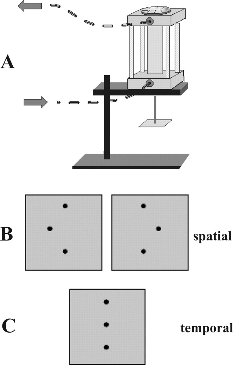
A, MRI-compatible pneumatic stimulator. Stimuli were mounted face-down on the square stage at the bottom of the drive shaft. The finger mold used to immobilize the finger was mounted on the base of the device. Arrows indicate direction of airflow. Disk on the top of the stimulator allowed 180° rotation of the stimulus. B, Stimulus configurations in spatial task; central dot in array was offset either to the right or left. C, Stimulus array for the temporal task used an array without spatial offset.

The tactile stimuli were plastic dot patterns raised 0.64 mm in relief from a square base plate of 20 mm side. They were produced by a commercial ultraviolet photo-etching process. The prototypical stimulus was a linear array of three dots (0.3 mm diameter, 2 mm center-to-center spacing) centered on the base plate. In the experimental stimulus array, the central dot was offset to the left or right (Fig. 1B) by a variable distance, ranging from 0.03 to 1.94 mm. A disk atop the stimulator allowed 180° rotation of a stimulus with a given offset to facilitate rapid switching between left and right offsets. Care was taken to ensure that the stimulus array was properly centered on the base plate so that this rotation would result in symmetric positioning of the two stimulus alternatives. The stimulus was applied to the finger pad for 1 s duration, and subjects were asked to determine whether the central dot was offset to the left or right. The control task used an array without an offset of the central dot (Fig. 1C), and stimulus duration was varied from 0.7 to 1.3 s (mean, 1 s). Subjects indicated whether the contact duration was long or short. Subjects were never allowed to see the stimuli, and they were instructed to keep their eyes closed during stimulation.

Prescanning psychophysical testing

Before MR scanning, each subject took part in a session in which their psychophysical thresholds were determined. Twenty-trial blocks of the experimental task were presented, in which the offset was constant within a block and there was an equal probability of left and right offsets. Testing began with the largest offset (1.94 mm) and continued until accuracy fell below 75% correct. Acuity thresholds were expressed in terms of the offset corresponding to 75% correct spatial discrimination, determined by linear interpolation between the two values immediately spanning 75% correct. For subsequent scanning with each subject, the offset value closest to that yielding 90% correct accuracy for that subject was chosen, with the objective of achieving performance during scanning that was above threshold but below ceiling. [One subject actually had a threshold of slightly over 1.94 mm (taken as 1.94 mm for analyses) but was included because her prescanning accuracy at the 1.94 mm offset was 70% correct, which is near threshold and well above chance.] Similarly, 20-trial blocks of the control task were administered, with each block containing a constant pair of stimulus durations and an equal probability of short and long durations. This testing began with the duration pair of 1.3 and 0.7 s and progressed to more difficult pairs (1.2 and 0.8 s, then 1.1 and 0.9 s) as necessary to select a pair that yielded ∼90% correct accuracy for use in subsequent scanning.

Functional imaging

Subjects lay supine in the scanner with the right arm extended and the right hand supinated. The arm was comfortably supported by foam padding, which also functioned to minimize transfer of gradient coil vibration to the upper extremity. The immobilized right index finger was centered relative to the pneumatic stimulator, which was positioned and stabilized at the scanner aperture by a vacuum bean bag. Foam blocks, as well as chin and forehead straps, were used to reduce head movement. Headphones were worn to convey audio cues and protect the subject's hearing.

A block design paradigm was used. Each functional run contained 12 stimulation blocks of 24 s duration: six experimental and six control blocks, presented in a pseudorandom order. Each stimulation block contained eight, 3 s trials. Thus, there were 48 trials of each condition per run. Each run began and ended with an 18 s baseline period; baseline intervals of 18 s also separated stimulation blocks. Immediately preceding each stimulation block, subjects heard the cues “offset” or “duration” to instruct them which task would follow. Baseline periods were preceded by the cue “rest.” Five subjects completed two runs per scan session, whereas each of the remaining 17 subjects completed four runs. Subjects held a two-button fiber-optic response box in the left hand and used the second or third digit to respond “right” or “left” during the experimental task or “long” or “short” during the control task. Stimulus presentation was controlled and responses recorded using Presentation software.

MR scans were performed on a 3 tesla Siemens Tim Trio whole-body scanner (Siemens Medical Solutions, Malvern, PA), using a standard quadrature head coil. T2*-weighted functional images were acquired using a single-shot gradient-recalled echo planar imaging sequence optimized for blood oxygenation level-dependent (BOLD) contrast. Twenty-one contiguous, axial slices of 5 mm thickness were acquired using the following parameters: repetition time (TR), 1500 ms; echo time (TE), 30 ms; field of view (FOV), 220 mm; flip angle (FA), 70°; in-plane resolution (IPR), 3.4 × 3.4 mm; in-plane matrix (IPM), 64 × 64. High-resolution anatomic images were acquired using a three-dimensional (3D) magnetization-prepared rapid gradient echo sequence (Mugler and Brookman, 1990) consisting of 176 contiguous, sagittal slices of 1 mm thickness (TR, 2300 ms; TE, 3.9 ms; inversion time, 1100 ms; FA, 8°; FOV, 256 mm; IPR, 1 × 1 mm; IPM, 256 × 256).

Analysis of imaging data

Preprocessing.

Image processing and analysis was performed using BrainVoyager QX version 1.6.3 (Brain Innovation, Maastricht, The Netherlands). Each subject's functional runs were real-time motion corrected using Siemens 3D-PACE (prospective acquisition motion correction). Functional images were preprocessed using sinc interpolation for slice scan time correction, trilinear-sinc interpolation for intrasession alignment (motion correction) of functional volumes, and high-pass temporal filtering to 1 Hz to remove slow drifts in the data. Anatomic 3D images were processed, coregistered with the functional data, and transformed into Talairach space (Talairach and Tournoux, 1988). Activations were localized with respect to 3D cortical anatomy with the aid of an MR sectional atlas (Duvernoy, 1999).

Generation of activation maps and correlations with behavior.

For group analysis, the transformed data were spatially smoothed with an isotropic Gaussian kernel (full-width half-maximum, 4 mm). Runs were normalized in terms of percentage signal change, to optimize preservation of differences between individual effect sizes. Statistical analysis of group data used random effects, general linear models followed by pairwise contrasts of the experimental and control conditions. Activation maps were corrected for multiple comparisons (q < 0.05) by the false discovery rate (FDR) approach (Genovese et al., 2002) implemented in BrainVoyager. Time course graphs of the BOLD signal were used to confirm task selectivity for all activations and distinguish between BOLD signal increases and decreases. ROIs were created for each activation site from the experimental (spatial) − control (temporal) contrast, centered on the “hotspots” and constrained to be no larger than 5 × 5 × 5 mm cubes. Within each ROI, the β weights for the experimental condition (relative to baseline) were determined for each subject. Taking these β weights as indices of activation strengths, linear correlations were run against spatial acuity threshold, across subjects.

Connectivity analyses.

The 22 subjects were divided into two groups: 10 subjects whose acuity threshold was below the median (<1.14 mm, “better” performers), and 12 subjects whose acuity threshold was at or above the median (≥1.14 mm, “poorer” performers). The imaging data from better performers was based on 38 functional runs; that from poorer performers was based on 40 functional runs. Effective connectivity patterns were derived, using Granger causality analyses, separately for each group and compared between the groups.

In the first step of Granger causality analysis, we used the BrainVoyager Granger causality plug-in that implements a bivariate autoregressive model to obtain Granger causality maps (GCMs) between a reference ROI and all other voxels in the brain (Roebroeck et al., 2005; Abler et al., 2006). We generated GCMs for each group using data from only the experimental task blocks, using as a reference the time course from the ROI whose activity was most highly correlated with acuity threshold, based on the correlational analysis outlined above. The time course data were averaged across the ROI and concatenated across subjects to increase statistical power. Because there were temporal discontinuities at the start of each task block and of each subject's data, and the predictive phase lag was equal to one TR, the first time point after each such discontinuity was omitted from the computations. A difference GCM was computed between the inputs to each voxel from the reference ROI and its outputs to the same reference ROI (Roebroeck et al., 2005). This GCM was thresholded using nonparametric bootstrapping of p values, by finding the fraction of extreme values in a surrogate null distribution created by recomputing each term for each voxel with a simulated null reference (from an autoregressive model estimated on the real reference) and FDR corrected for multiple comparisons (q < 0.01).

Although such bivariate Granger causality analysis can provide useful information, it cannot model simultaneous interactions between more than two ROIs. We therefore augmented the bivariate approach by a subsequent multivariate analysis of Granger causality, for which ROIs were selected to be representative of those activated on the experimental − control contrast and also included some identified on the bivariate GCM. The entire time series of BOLD signal intensities from these selected ROIs, averaged across voxels within each ROI, were normalized across runs and subjects and concatenated across all runs and subjects (separately for each group) to form a single vector per ROI. Multivariate Granger causality analysis used the directed transfer function (DTF), computed from a multivariate autoregressive model of the time series in the selected ROIs. This method has been validated previously using simulations (Kus et al., 2004) and applied successfully to electrophysiological data (Ding et al., 2000; Kaminski et al., 2001; Korzeniewska et al., 2003; Blinowska et al., 2004; Kus et al., 2004). The DTF is based on the principle of Granger causality but is rendered in a multivariate formulation (Blinowska et al., 2004) and hence can effectively model the inherently multivariate nature of neuronal networks. The procedure has been used recently in multivariate analysis of connectivity patterns in fMRI data (Deshpande et al., 2006a,b) (G. Deshpande, S. LaConte, A. James, S. Peltier, and X. Hu, unpublished observations). Here, we weighted DTF with partial coherence to emphasize direct connections and suppress mediated influences. The output of the DTF analysis is a set of path weights representing the strength of drive, in arbitrary units, from each ROI to each of the other ROIs. For bivariate analyses, these path weights are typically normalized; however, if such a normalization procedure is performed for each ROI, comparisons between path weights of different ROIs would be rendered meaningless. Therefore, the path weights were not normalized in the present study. Surrogate null distributions were used to assess the significance of the path weights (p < 0.05). Because this analysis was performed on selected ROIs that survived correction for multiple comparisons in previous analyses, additional significance correction was not performed. Details of the method are given in Appendix.

Results

Psychophysical data

Spatial acuity thresholds ranged from 0.63 to 1.94 mm (mean ± SEM, 1.15 ± 0.07 mm). Mean ± SEM accuracy during scanning was 80.0 ± 2.6% for the experimental (spatial) task and 88.4 ± 1.1% for the control (temporal) task. The accuracy difference favoring the temporal task was significant on a paired t test (t₍₂₁₎ = −3.16; p = 0.005).

Activations

A number of regions were more active during the experimental (spatial) task compared with the control (temporal) task, as shown in Figure 2 and Table 1. These regions included the following: the aIPS, posterior IPS (pIPS), precuneus, posterior insula, lateral occipital complex (LOC), and FEFs bilaterally; the PCS, a lateral inferior parietal focus, the PMv, and inferior frontal sulcus on the left; and the right parietal operculum. In addition to these cerebral cortical regions, the thalamus was active bilaterally. Although thalamic activations are more difficult to localize specifically, especially on smoothed, grouped data, reference to the atlas suggested that they included the (somatosensory) ventral posterolateral nucleus bilaterally and the left mediodorsal nucleus. Figure 3 illustrates representative BOLD signal time courses from the spatial task-related activations of Figure 2. It is worth noting in Figure 3 that LOC activation in the spatial task was minimal. In this region as well as in other regions such as the right pIPS and right precuneus, an early increase in BOLD signal was followed by a substantial decrease below baseline.

Figure 2.

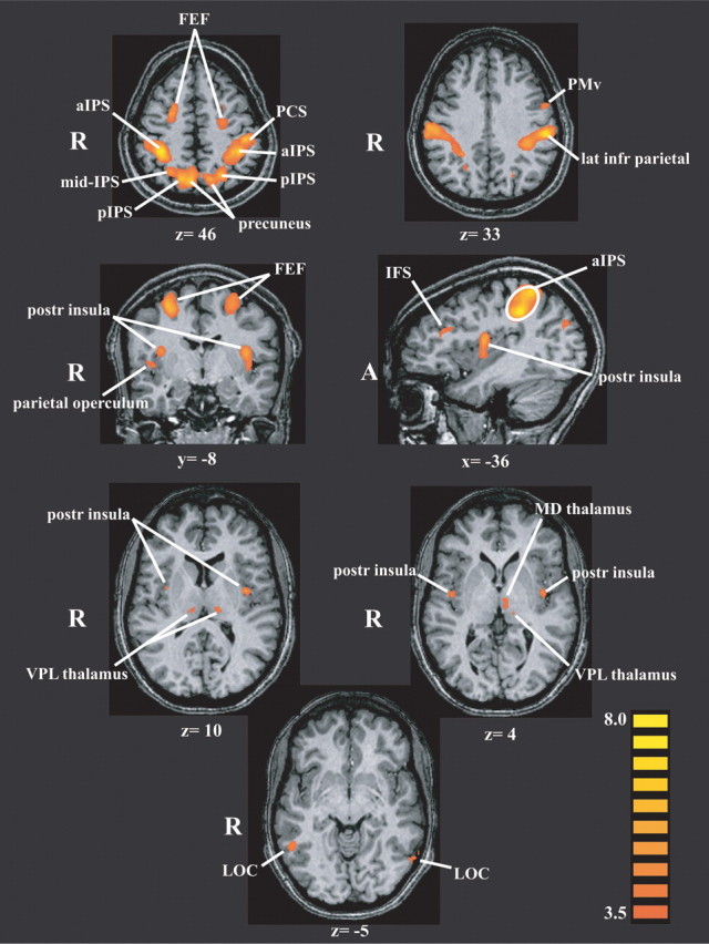
Activations in the 22-subject group on the spatial task relative to the temporal task, displayed on representative slices through the anatomic images from one subject using a pseudocolor t scale. Values below each slice indicate its Talairach plane. Activations are derived from a random-effects analysis and FDR corrected for multiple comparisons (q < 0.05). R, Right; A, anterior; IFS, inferior frontal sulcus; MD, mediodorsal; VPL, ventral posterolateral.

Table 1.

Talairach coordinates (x, y, z) and peak t values of activations on spatial–temporal contrast (top) and temporal–spatial contrast (bottom)

	x	y	z	tmax	r	p
Spatial > temporal
L FEF	−26	−13	60	7.1	−0.02	0.91
R FEF	29	−8	54	6.6	−0.03	0.89
L IFS	−34	25	23	4.6	−0.15	0.5
L PMv	−52	1	33	4.6	−0.09	0.68
L lateral inferior parietal	−53	−26	33	8.1	0.24	0.27
L PCS	−44	−28	44	7	0.005	0.98
L aIPS	−34	−38	38	8.8	0.17	0.44
L pIPS	−22	−62	48	6.6	0.21	0.34
L precuneus	−14	−69	49	6.4	−0.27	0.23
R aIPS	36	−41	42	9.2	0.06	0.8
R mIPS	27	−60	46	5.2	−0.19	0.39
R pIPS	16	−67	46	6.6	−0.56	0.007
R precuneus	7	−67	47	7.2	−0.42	0.0496
L posterior insula	−35	−7	13	6	−0.32	0.15
R posterior insula	35	−5	16	6.6	−0.26	0.25
R parietal operculum	42	−8	6	4.3	−0.11	0.64
L VPL thalamus	−11	−23	10	4.5	0.16	0.48
L MD thalamus	−5	−17	4	4.2	0.36	0.096
R VPL thalamus	11	−23	11	3.9	−0.03	0.9
L LOC	−54	−61	−5	4	−0.03	0.88
R LOC	50	−51	−5	4.7	−0.05	0.81
Temporal > spatial
SMA/pre-SMA	5	2	59	4.8
L MFG	−32	39	33	−4.8

Last two columns give linear correlation coefficients (r) and p values for correlations across subjects between acuity threshold and β weight of activation for each ROI on the spatial task relative to baseline. Values in bold indicate significant correlations (p < 0.05). L, Left; R, right; IFS, inferior frontal sulcus; mIPS, mid-intraparietal sulcus; VPL, ventral posterolateral; MD, mediodorsal; MFG, middle frontal gyrus.

Figure 3.

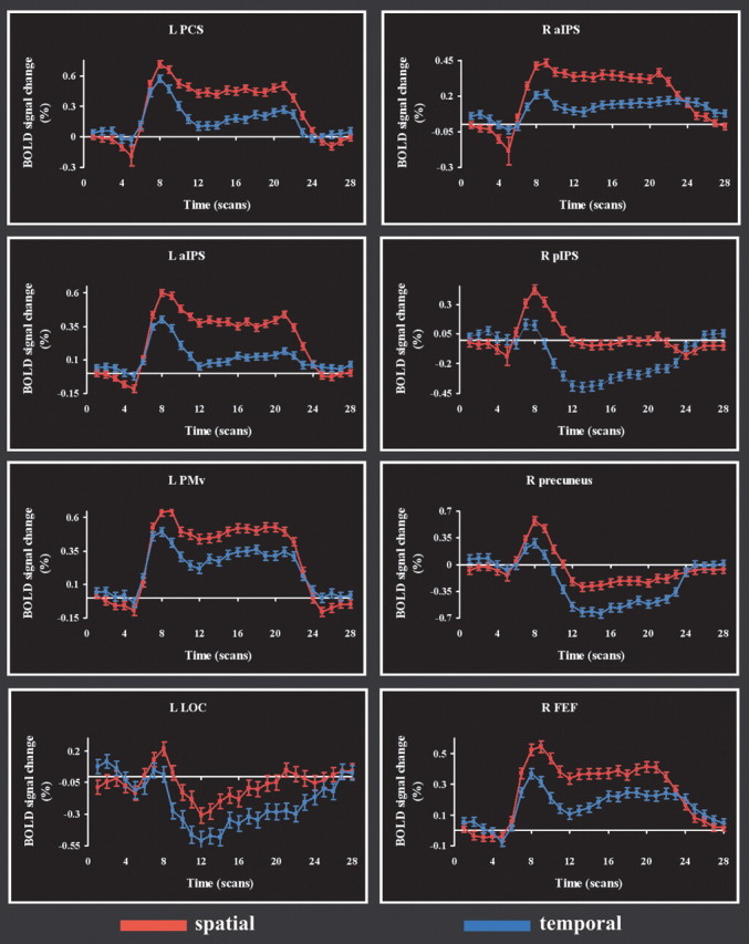
Time courses of BOLD signal change in representative regions that were more active on the spatial task than the temporal task. Abbreviations as in Figure 2. The horizontal (time) axis is calibrated in terms of scan number (TR, 1.5 s). R, Right; L, left.

Regions more active in the temporal task relative to the spatial task were the supplementary motor area (SMA) extending into the pre-SMA, and the left middle frontal gyrus, as shown in Figure 4 and Table 1. Figure 4 also shows the BOLD signal time courses from the temporal task-related activations.

Figure 4.

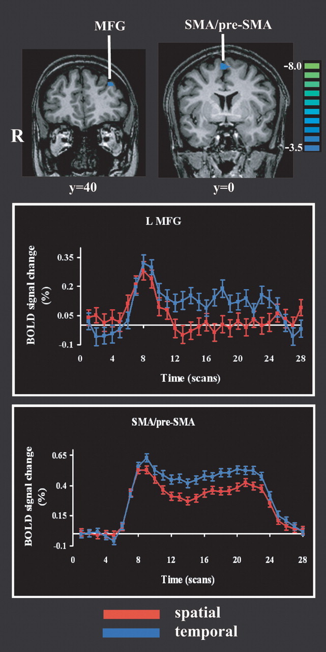
Activations on the temporal task relative to the spatial task and their time courses. Details are as in Figures 2 and 3. MFG, Middle frontal gyrus; R, right; L, left.

Correlations between activation strengths and acuity thresholds

Table 1 lists, for each ROI active on the spatial task relative to the temporal control, the linear correlation coefficient across subjects between the β weights in that ROI (for the spatial task relative to baseline) and the psychophysically measured acuity threshold. Only two ROIs showed significant correlations: the right pIPS (r = −0.56; p = 0.007) and the right precuneus (r = −0.42; p = 0.05); it is apparent from Figure 2 that these two regions are juxtaposed within right posteromedial parietal cortex. The negative correlations indicate that higher β weights (stronger activations) were associated with lower acuity thresholds, which correspond to better performance.

Connectivity analyses

Bivariate Granger causality analysis

Because the right pIPS showed the highest correlation with acuity, it was chosen as a seed for the initial, bivariate analysis of Granger causality. GCMs were computed, separately for each group, for the data derived from the spatial condition alone, using the right pIPS as the reference ROI. The resulting GCMs are shown in Figure 5. For both groups, the GCMs were dominated by input connections arising from essentially all the regions showing spatial task-specific activity (compare Figs. 2, 5, particularly slices at z = 46, y = −8/−5), with additional inputs arising from medial parietal and medial occipital cortex, as well as deep gray matter of the hemispheres. The net outputs from this region were much sparser and directed mainly into inferior occipital cortex and precuneus. The GCMs suggest more extensive connectivity of the right pIPS ROI in the better performers compared with the poorer performers.

Figure 5.

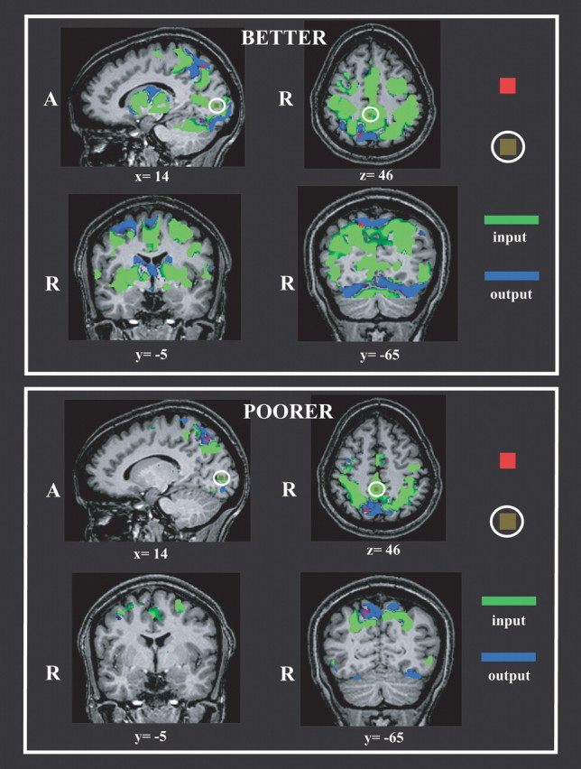
Bivariate Granger causality maps using the right pIPS ROI (red) as a reference. Representative slices are illustrated. Top, Better performers. Bottom, Poorer performers. Olive-green ROIs within white ellipses indicate location of medial parietal and right calcarine ROIs selected from these maps for subsequent multivariate Granger causality analyses. A, Anterior; R, right.

Multivariate Granger causality analysis

Nine representative ROIs were selected for the subsequent multivariate analysis of Granger causality. Seven of these were regions showing spatial task-selective activation: the pIPS, aIPS, and FEF bilaterally and the left PCS. In addition, two ROIs were selected from the bivariate GCMs. One was in right calcarine cortex, presumably in or near primary visual cortex, and the other was in medial parietal cortex (Fig. 5). The calcarine ROI exhibited minimal, nonselective activation during both spatial and temporal tasks; the medial parietal ROI was nonselectively deactivated (i.e., negative BOLD signal change), consistent with its location in the “default network” (Raichle et al., 2001). A multivariate analysis of Granger causality was performed on the time series from these nine ROIs, separately for each group. Figure 6 displays the results, using a pseudocolor code to indicate the path weights of all possible connections between these nine ROIs. The path weights are tabulated in Table 2, with significant connections shown in bold type. The arrows beside each path weight reflect the tendency of the BOLD signal in the two ROIs linked by the path to covary in the same direction, i.e., both tending to increase or decrease together (↑), albeit with a phase difference, or vary in opposite directions, i.e., one tending to increase when the other tends to decrease (↓), analogous to positive and negative correlations. For the sake of simplicity, these are henceforth referred to as “covarying” and “antivarying” paths, but this terminology should not be taken to imply excitatory versus inhibitory connections at the neuronal level, because our inferences of Granger causality are based on the hemodynamic response, whose relationship with excitatory versus inhibitory synaptic activity is still unsettled. A two-way ANOVA was used to confirm that the connectivity matrices shown in Table 2 were indeed different between the better and poorer performers. The ANOVA confirmed a significant effect of group (F₍₁₎ = 5.99; p = 0.02) as well as path (F₍₇₁₎ = 3.67; p = 15 × 10⁻¹⁵). Figure 7 illustrates the paths whose weights significantly differed between groups (p < 0.05), as established by the use of surrogate null distributions (see Appendix).

Figure 6.

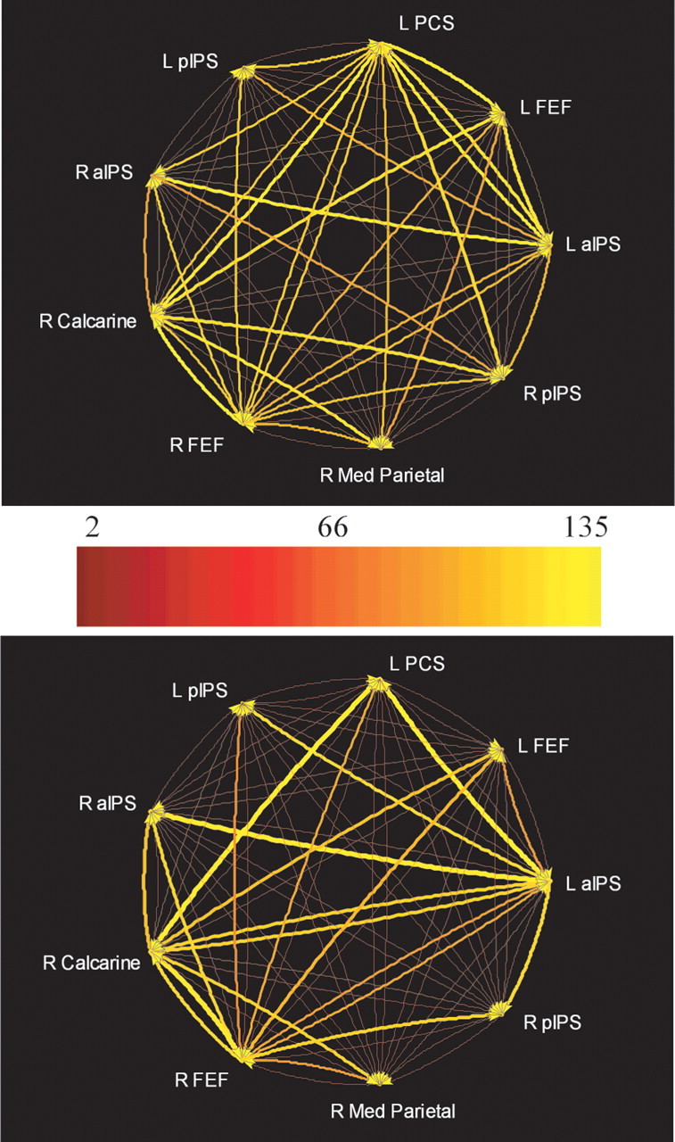
Multivariate Granger causality relationships among selected ROIs (for details of selection, see Results) in better (top) and poorer (bottom) performers. Relative strength of path weights (in arbitrary units) is indicated by a pseudocolor code. The actual path weights are tabulated in Table 2. L, Left; R, right.

Table 2.

Path weights (arbitrary units) from multivariate Granger causality analyses in better (top) and poorer (bottom) performers

	L aIPS	L FEF	L PCS	L pIPS	R aIPS	R calcarine	R FEF	R medial parietal	R pIPS
Better
L aIPS		51↓	97↑	18↑	50↓	29↑	71↑	20↑	4↑
L FEF	98↑		101↑	16↑	48↑	95↑	69↑	22↓	7↑
L PCS	105↑	44↓		21↑	45↓	82↑	83↑	25↑	10↓
L pIPS	67↑	30↑	86↑		29↑	36↑	85↑	38↑	19↓
R aIPS	101↑	50↓	86↑	14↑		60↑	87↑	6↓	4↑
R calcarine	32↑	49↓	101↑	11↑	43↓		105↑	38↑	22↓
R FEF	76↑	36↓	84↑	26↑	51↓	82↑		19↓	4↑
R medial parietal	55↑	60↓	76↑	19↑	16↑	97↑	74↑		7↑
R pIPS	74↑	33↑	91↑	16↑	62↑	94↑	80↑	25↑
Poorer
L aIPS		10↑	3↑	27↑	9↑	111↑	76↑	4↓	14↓
L FEF	72↑		3↓	18↑	12↑	102↑	91↑	17↑	7↑
L PCS	135↑	10↑		18↑	7↓	130↑	83↑	12↓	7↑
L pIPS	119↑	14↑	5↓		2↓	60↑	64↑	19↑	14↓
R aIPS	129↑	21↑	10↓	7↑		99↑	113↑	12↓	16↓
R calcarine	112↑	15↑	6↑	10↓	5↓		117↑	20↑	2↑
R FEF	85↑	17↑	2↓	13↑	14↑	125↑		12↑	10↓
R medial parietal	43↑	14↑	4↓	24↑	6↓	111↑	74↑		6↑
R pIPS	116↑	24↑	10↓	17↑	6↓	45↑	110↑	25↑

Significant weights are indicated in bold type. Arrows beside each path weight reflect covariations in the same direction (↑) or opposite direction (↓). L, Left; R, right.

Figure 7.

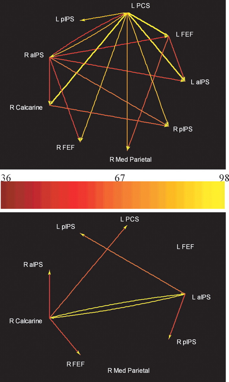
Paths differing significantly between better and poorer groups on multivariate Granger causality analyses. Top, Better > poorer; bottom, poorer > better. L, Left; R, right.

A few points emerge from consideration of the results of these multivariate analyses. (1) The connectivity pattern was much more balanced in the better group compared with the poorer group. (2) The left PCS and left FEF were important sources in the better group but tended to be targets in the poorer group. Paths originating in the left PCS were all linked to strongly covarying ROIs in the better group, but weakly linked, and mostly to antivarying ROIs in the poorer group. Paths arising from the left FEF were mostly to antivarying ROIs in the better group but to covarying ROIs in the poorer group. (3) The right aIPS, which was relatively balanced with respect to inputs and outputs in the better group, was more of a target than source in the poorer group. (4) In the better group, significant drive to the right pIPS was relatively balanced, deriving from five of the other six spatial task-selective ROIs (all except its counterpart in the left hemisphere), whereas in the poorer group, the right pIPS was driven significantly from only three of the spatial task-selective ROIs (the left aIPS and the FEF bilaterally). (5) There was significant covarying drive from the left aIPS, right FEF, and right calcarine foci to all other ROIs tested in both groups.

Correlations between path weights and acuity thresholds

We asked which of the paths shown in Figure 6 significantly predicted performance, using stepwise regression (Draper and Smith, 1981). There were two in each group: for the better group, the path from the left PCS to the right pIPS was most predictive; that from the right FEF to the right pIPS was the next most predictive (Table 3). Both these paths linked covarying ROIs whose BOLD signal tended to rise or fall together, with strengths correlating negatively with acuity threshold (i.e., stronger covarying path weights were associated with lower thresholds and thus better performance). Together, these two path weights accounted for 86% of the variance in acuity threshold in the better group (F₍₂₎ = 33.6; p = 3.8 × 10⁻⁴). For the poorer group, the paths predictive of performance were both positively correlated with acuity threshold (i.e., stronger path weights were associated with higher thresholds and thus poorer performance). These paths were from the left PCS to the left pIPS (an antivarying path that actually had a nonsignificant weight) and from the right FEF to the right aIPS (a covarying path with a significant weight). These two paths together accounted for 93% of the variance in acuity threshold in the poorer group (F₍₂₎ = 59.4; p = 6.5 × 10⁻⁶). Note that, in both groups, the paths predicting performance derived from common sources: whereas the two paths converged on a single target in the better group, which was the ROI most highly correlated with performance, they were nonconvergent paths directed at different targets in the poorer group.

Table 3.

Stepwise regression statistics for paths from multivariate Granger causality analyses that significantly predicted acuity thresholds

	Path	t	p	Progressive R2
Better	L PCS → R pIPS	−6.55	3.0 × 10−4	0.59
	R FEF → R pIPS	−3.67	7.9 × 10−3	0.86
Poorer	L PCS → L pIPS	9.06	0	0.63
	R FEF → R aIPS	6.22	2.0 × 10−4	0.93

L, Left; R, right.

Task specificity of path weights

To address whether the connectivity patterns were specific to the spatial task compared with the temporal task, we calculated the task-specific path weights for the two connections that best predicted behavior (left PCS to right pIPS and right FEF to right pIPS, the two paths whose weights correlated best with acuity threshold in the better group) on a subject-by-subject basis. Two-way ANOVAs were performed, with subject and task as factors, the two connections being considered as different observations for each subject and task. Because the two paths were important in the better but not the poorer group, a separate ANOVA was run for each group. The effect of subject was not significant in either group, indicating consistency across subjects (better group, F₍₉₎ = 1.2, p = 0.33; poorer group, F₍₁₁₎ = 1.9, p = 0.07). The effect of task was significant in the better group (F₍₁₎ = 4.1; p = 0.02), with the mean path weight being higher for the spatial than the temporal task, but not in the poorer group (F₍₁₎ = 1.35; p = 0.27). Thus, the connections of interest were specific for the spatial task in the better group.

Correlations between activation strengths and path weights

Finally, we addressed the relationship between activations and connectivity by performing a multiple regression between the two connections best predicting acuity threshold in the better group (left PCS to right pIPS and right FEF to right pIPS) and the β weights in the right pIPS. The fit of the resulting model to the data were significant in the case of the better group (R² = 0.51; F = 8.78; p = 0.01) but not for the poorer group (R² = 0.26; F = 3.2; p = 0.1). Across the entire 22-subject group, the fit was nearly significant (R² = 0.15; F = 3.8; p = 0.06). In each case, the path weights correlated positively with the β weights, with the exception of the right FEF to right pIPS path in the poorer group, in which the correlation was in the negative direction. Overall, this analysis indicates that greater activation in the right pIPS focus was accompanied by stronger drive from the left PCS and right FEF, particularly in the better group.

Discussion

Psychophysical considerations

The mean acuity threshold at the right index finger pad in the present study, 1.15 mm, was very similar to that observed at the same site in a number of other studies using different tests (Table 4). Although there was a significant difference in accuracy during imaging between the spatial (experimental) and temporal (control) tasks, this difference was small and seems unlikely to account for task-related activations. Critically, the relationships of individual subjects' activation magnitudes and connectivity patterns to their acuity thresholds indicate the behavioral importance of our imaging findings. It is important to note that the stimulus parameters used during imaging were individualized based on subjects' acuity thresholds and that correlations of imaging data were examined in relation to these thresholds.

Table 4.

Tactile spatial acuity at the right index finger pad as measured in previous studies

Acuity threshold (mm)	Test used	Reference
0.87	Gap detection (m)	Johnson and Phillips, 1981
	Grating orientation
0.84	discrimination (m)	Johnson and Phillips, 1981
	Grating orientation
0.98	discrimination (h)	Van Boven and Johnson, 1994
	Grating orientation
0.96	discrimination (h)	Sathian and Zangaladze, 1996
	Grating orientation
1.23	discrimination (h)	Vega-Bermudez and Johnson, 2001
	Grating orientation
1.06	discrimination (h)	Grant et al., 2006

m, Mechanized stimulator used; h, hand-held stimulus.

Tactile spatial processing

Regions identified on the spatial − temporal contrast can be regarded as being active specifically during fine spatial processing of tactile stimuli, because both low-level somatosensory and motor processing and high-level cognitive processes associated with attention and decision processes were subtracted out. This contrast demonstrated activation of parietal, occipital, and frontal cortical areas as well as thalamic regions.

Sensory cortex

Some of the regions selective for spatial processing were in classical somatosensory cortex: the left PCS, a right parietal opercular focus, and bilateral foci in the posterior insula. The PCS corresponds to Brodmann's area 2 of SI (Grefkes et al., 2001). The lack of task-specific activation in more anterior parts of SI does not negate a role for these regions in tactile spatial processing; indeed, neurophysiological evidence in monkeys clearly implicates neurons in area 3b (Phillips et al., 1988), and human tactile hyperacuity, as measured on a task very similar to that of the present study, scales with the cortical magnification factor in SI (Duncan and Boynton, 2007). Presumably, these regions are involved in the basic somatosensory processing underlying both the spatial and the temporal task.

The parietal operculum, in which SII is located, contains multiple somatosensory fields in both monkeys (Fitzgerald et al., 2004) and humans (Eickhoff et al., 2006a,b). In humans, there are three somatosensory fields, termed OP1, OP3, and OP4 (Eickhoff et al., 2007). The posterior insular and right parietal opercular foci of the present study appeared to lie entirely within the OP3 region, which is probably homologous to the ventral somatosensory area of monkeys (Eickhoff et al., 2007). Given that texture depends on fine spatial detail, the selectivity of this region for fine spatial processing in the present study fits with the texture selectivity reported in the parietal operculum (Roland et al., 1998; Stilla and Sathian, 2007), which spans all three of its somatosensory fields (Stilla and Sathian, 2007). However, fine spatial processing in the present study also recruited multisensory areas that are shape-selective during both haptic and visual perception: the aIPS, pIPS, and LOC bilaterally, and the left PCS (Peltier et al., 2007; Stilla and Sathian, 2007). Among these areas, activation in the LOC was minimal, consistent with LOC activation during tactile perception in macrospatial but not microspatial tasks (Stoesz et al., 2003). Furthermore, the ventral IPS (vIPS), another visuohaptic shape-selective area (Peltier et al., 2007; Stilla and Sathian, 2007) was not active in the present study. Thus, it appears that the neural networks mediating macrospatial and microspatial form processing are partially overlapping, in the aIPS and pIPS, and partially segregated: macrospatial processing engages the PCS, vIPS, and LOC, whereas microspatial processing engages parietal opercular–insular cortex.

Premotor cortex

Interestingly, selective activations in the spatial task relative to the control task were observed in frontal cortical areas generally regarded as premotor: the left PMv and bilateral FEF. These activations cannot be attributed to preparation or execution of motor output, because identical motor responses were emitted in both tasks. Decision processes, which can engage premotor cortical regions (Romo and Salinas, 2003), are also unlikely to explain these activations, unless such processes were specific to the spatial task. Thus, these regions may be specifically involved in some aspect of tactile spatial processing. There is evidence that both the PMv and FEF have multisensory inputs, combining visual–somatosensory responsiveness in the case of the PMv (Graziano et al., 1997) and visual–auditory responsiveness in the case of the FEF (Russo and Bruce, 1989). However, their role in sensory processing remains to be defined.

Behavioral relationships

Of all the regions that were selective for fine spatial processing, the only two whose activation magnitude significantly predicted psychophysically measured acuity were located near each other, in right posteromedial parietal cortex. Higher levels of activity in these regions were associated with better acuity. The highest correlation with acuity was in the right pIPS; a somewhat lower correlation was found in the precuneus. Intriguingly, these loci were ipsilateral to the stimulated finger and outside classical somatosensory cortex. Both these regions are more active during sensorimotor tracking of visuospatial compared with vibrotactile stimuli (Meehan and Staines, 2007). The pIPS is among the bisensory (visuohaptic) regions recruited bilaterally during shape perception (Peltier et al., 2007; Stilla and Sathian, 2007) and was specifically engaged during visuotactile matching of shape patterns on Mah Jong tiles (Saito et al., 2003). A nearby focus was also reported to be active during visual discrimination of surface orientation (Shikata et al., 2001, 2003). Together, these previous findings suggest that the activation of posteromedial parietal cortex in the present study, which appears to favor better tactile spatial acuity, could reflect either a visualization strategy or engagement of a modality-independent spatial processor.

Connectivity patterns

The bivariate GCMs suggested that the right pIPS was an important site of convergence of inputs from other regions that were selective for tactile spatial processing, from regions located in the default network, and from pericalcarine cortex. Outputs from the right pIPS to other brain regions were much sparser than its inputs. Connections to and from this focus were more extensive in individuals with better tactile spatial acuity. The multivariate analysis of Granger causality corroborated these findings and extended them by showing that the pattern of inputs to the right pIPS was more balanced in the better performers than the poorer performers. Together, both types of Granger causality analysis provide additional support for a pivotal role of the right pIPS in the neural processing underlying fine tactile spatial discrimination.

The overall multivariate pattern of connectivity was also more balanced in the better performers than the poorer performers, and there were a number of specific differences between groups. It is interesting that the PCS, which has been equated to Brodmann's area 2 of SI (Grefkes et al., 2001) and is thus at the lowest hierarchical level of the activations seen in the present study, was a more important source in the better group than the poorer group. Moreover, the path from the left PCS to the right pIPS was the strongest predictor of acuity threshold in the better group, suggesting that the optimal strategy for the tactile spatial task used here relies on strong inputs from SI to the right pIPS. The role of the next strongest predictor of acuity threshold in the better group, the path from the right FEF to the right pIPS, is less clear but may reflect a top-down control signal, possibly related to spatially focused attention, given the evidence for involvement of these regions in visual spatial attention (Corbetta and Shulman, 2002). The convergence of both these key paths on the right pIPS focus, with stronger covarying path weights being associated with both better acuity and stronger activation of this focus, and their specificity for the spatial task in the better group, all reinforce the critical role of the right pIPS focus in fine tactile spatial processing. We propose that this convergence represents top-down control, possibly via spatial attention, of mechanisms involving either visualization of the spatial configurations of tactile stimuli or engagement of a modality-independent spatial processing network, and that the successful operation of these mechanisms underlies facility with perceptual discrimination.

In contrast, in the poorer group, the paths that best predicted acuity were associated with worsening acuity as path strength increased. The paths emanated from the same ROIs as in the better group, but instead of converging on one focus, drove different regions in the poorer group: a relatively weak, antivarying path from the left PCS to the left pIPS and a covarying path from the right FEF to the right aIPS. The left PCS, left FEF, and right aIPS differed in connectivity between groups, tending to be targets in the poorer group compared with being sources (left PCS, left FEF) or having more balanced inputs and outputs (right aIPS) in the better group. Another set of ROIs, the left aIPS, right FEF, and right calcarine, had similar patterns of connectivity in both groups, being significant sources. The right calcarine source might suggest a role for visualization; however, the lack of group specificity of its outputs, and of task specificity of its activity level, implies that such a role, if it exists, is nonspecific and unlikely to be of functional relevance. A similar inference might be made for the weak, nonselective tactile activation observed by others in primary visual cortex of normally sighted subjects (Merabet et al., 2007).

Tactile temporal processing

Although this was not our primary interest in the present study, our finding of temporally specific activation for touch in the pre-SMA replicates that reported in a previous study (Pastor et al., 2004). In the present study, the pre-SMA activation extended posteriorly into the SMA; the division between these two regions corresponds to y = 0, i.e., the coronal plane of the anterior commissure (Picard and Strick, 2001).

Conclusions

We conclude that fine tactile spatial discrimination near the limit of acuity recruits activity in a distributed neural network that includes parietal and frontal cortical areas. Across subjects, the level of activity in right posteromedial parietal cortical foci, the pIPS and precuneus, predict acuity thresholds. Connectivity patterns differ in many respects between better and poorer performers, including the strength of inputs into the right pIPS. In better performers, the paths predicting acuity converge from the left PCS and right FEF onto the right pIPS. These paths are stronger during performance of the spatial compared with the temporal task, and their strengths also predict the level of activity in the right pIPS. We propose that the optimal strategy for fine tactile spatial discrimination involves interaction in the pIPS of a top-down control signal, possibly attentional, with somatosensory cortical inputs, reflecting either visualization of the spatial configurations of tactile stimuli or engagement of a specialized spatial processing circuit that is modality independent.

Appendix

Multivariate Granger causality-based effective connectivity

Effective connectivity was examined using a multivariate autoregressive model (MVAR) (Kaminski et al., 2001). Our specific approach was as follows. Let X(t) = [x₁(t),x₂(t)… x_Q(t)] be a matrix representing data from Q ROIs, in which each column is an ROI time series. The MVAR model of order p is given by the following:

where E(t) is the vector corresponding to the residual errors. The Akaike information criterion was used to determine model order (Akaike, 1974); a model order of 1 (corresponding to one TR) was chosen (the same as used in the bivariate implementation in BrainVoyager). A(n) is the matrix of prediction coefficients composed of elements a_ij(n). The Fourier transform of Equation 1 is as follows:

where

δ_ij is the Dirac-delta function, which is 1 when i = j and 0 otherwise. Also, i = 1…Q, j = 1…Q. h_ij(f), the element in the ith row and jth column of the frequency domain transfer matrix H(f), is referred to as the non-normalized DTF (Kus et al., 2004) corresponding to the influence of ROI j onto ROI i. h_ij(f) was multiplied by the partial coherence between ROIs i and j to obtain the direct DTF (dDTF) (Kus et al., 2004) (Deshpande, LaConte, James, Peltier, and Hu, unpublished observations). This procedure ensures that direct connections are emphasized and mediated influences are de-emphasized. To calculate the partial coherence, the cross-spectra were computed as follows:

where V is the variance of the matrix E(f), and the asterisk denotes transposition and complex conjugation. The partial coherence between ROIs i and j is then given by the following:

where M_ij(f) is the minor obtained by removing the ith row and jth column from the matrix S (Strang, 1998). The partial coherence lies in the range of [0, 1] in which a value of 0 (1) indicates no direct (complete) association between the ROIs with the influence of all other ROIs removed. It is analogous to partial correlation in the frequency domain. The sum of all frequency components of the product of the non-normalized DTF and partial coherence was defined as the dDTF:

The value of dDTF only reflects the magnitude of causal influence between the ROIs. Causal influence could potentially arise either because of “covarying” or “antivarying” phase relationships between time series. This information was inferred by the sign of the predictor coefficients a_ij(n), which are indicated as up (covarying) or down (antivarying) arrows in Table 2.

Statistical significance testing

In the absence of established analytical distributions of multivariate Granger causality (Kaminski et al., 2001), we used surrogate data (Theiler et al., 1992; Kaminski et al., 2001; Kus et al., 2004) to obtain an empirical null distribution to assess the significance of the causality indicated by dDTF. Surrogate time series were generated by transforming the original time series into the frequency domain and randomizing their phase to be uniformly distributed over (−π, π) (Kus et al., 2004). Subsequently, the signal was transformed back to the time domain to generate surrogate data with the same frequency content as the original time series but with the causal phase relations destroyed. The dDTF matrix was computed by inputting the surrogate time series of each ROI into the MVAR model instead of the original time series. This procedure was repeated 2500 times to obtain a null distribution for every connection in the dDTF matrix. For each connection, its null distribution was used to ascertain a p value for its dDTF value derived from the experimental data. For testing the statistical significance of the difference between connectivity values of the better and poorer groups, the same procedure described above was used with the difference matrix replacing the dDTF matrix.

References

- Abler B, Roebroeck A, Goebel R, Hose A, Schoenfeldt-Lecuona C, Hole G, Walter H. Investigating directed influences between activated brain areas in a motor-response task using fMRI. Magn Reson Imaging. 2006;24:181–185. doi: 10.1016/j.mri.2005.10.022. [DOI] [PubMed] [Google Scholar]
- Akaike H. A new look at the statistical model identification. IEEE Trans Autom Control. 1974;19:716–723. [Google Scholar]
- Blinowska KJ, Kus R, Kaminski M. Granger causality and information flow in multivariate processes. Phys Rev E. 2004;70:50902–50906. doi: 10.1103/PhysRevE.70.050902. [DOI] [PubMed] [Google Scholar]
- Büchel C, Friston K. Extracting brain connectivity. In: Jezzard P, Matthews PM, Smith SM, editors. Functional MRI. An introduction to methods. Oxford: Oxford UP; 2001. pp. 295–308. [Google Scholar]
- Corbetta M, Shulman GL. Control of goal-directed and stimulus-driven attention in the brain. Nat Rev Neurosci. 2002;3:201–215. doi: 10.1038/nrn755. [DOI] [PubMed] [Google Scholar]
- Deshpande G, LaConte S, Peltier S, Hu X. Directed transfer function analysis of fMRI data to investigate network dynamics. Proceedings of the 28th Annual International Conference of the Institute of Electrical and Electronics Engineers Engineering in Medicine and Biology Society; August–September; New York. 2006a. [DOI] [PubMed] [Google Scholar]
- Deshpande G, LaConte S, Peltier S, Hu X. Investigating effective connectivity in cerebro-cerebellar networks during motor learning using directed transfer function. 12th Annual Human Brain Mapping Meeting. NeuroImage. 2006b;31(Suppl 40) [Google Scholar]
- DiCarlo JJ, Johnson KO, Hsiao SS. Structure of receptive fields in area 3b of primary somatosensory cortex in the alert monkey. J Neurosci. 1998;18:2626–2645. doi: 10.1523/JNEUROSCI.18-07-02626.1998. [DOI] [PMC free article] [PubMed] [Google Scholar]
- Ding M, Bressler SL, Yang W, Liang H. Short-window spectral analysis of cortical event-related potentials by adaptive multivariate autoregressive modeling: Data preprocessing, model validation, and variability assessment. Biol Cyber. 2000;83:35–45. doi: 10.1007/s004229900137. [DOI] [PubMed] [Google Scholar]
- Draper NR, Smith H. Applied regression analysis. New York: Wiley Interscience; 1981. [Google Scholar]
- Duncan RO, Boynton GM. Tactile hyperacuity thresholds correlate with finger maps in primary somatosensory cortex (S1) Cereb Cortex. 2007 doi: 10.1093/cercor/bhm015. in press. [DOI] [PubMed] [Google Scholar]
- Duvernoy HM. Surface, blood supply and three-dimensional sectional anatomy. New York: Springer; 1999. The human brain. [Google Scholar]
- Eickhoff SB, Schleicher A, Zilles K, Amunts K. The human parietal operculum. I. Cytoarchitectonic mapping of subdivisions. Cereb Cortex. 2006a;16:254–267. doi: 10.1093/cercor/bhi105. [DOI] [PubMed] [Google Scholar]
- Eickhoff SB, Amunts K, Mohlberg H, Zilles K. The human parietal operculum. II. Stereotaxic maps and correlation with functional imaging results. Cereb Cortex. 2006b;16:268–279. doi: 10.1093/cercor/bhi106. [DOI] [PubMed] [Google Scholar]
- Eickhoff SB, Grefkes C, Zilles K, Fink GR. The somatotopic organization of cytoarchitectonic areas on the human parietal operculum. Cereb Cortex. 2007;17:1800–1811. doi: 10.1093/cercor/bhl090. [DOI] [PubMed] [Google Scholar]
- Fitzgerald PJ, Lane JW, Thakur PH, Hsiao SS. Receptive field properties of the macaque second somatosensory cortex: evidence for multiple functional representations. J Neurosci. 2004;24:11193–11204. doi: 10.1523/JNEUROSCI.3481-04.2004. [DOI] [PMC free article] [PubMed] [Google Scholar]
- Fitzgerald PJ, Lane JW, Thakur PH, Hsiao SS. Receptive field (RF) properties of the macaque second somatosensory cortex: RF size, shape, and somatotopic organization. J Neurosci. 2006;26:6485–6495. doi: 10.1523/JNEUROSCI.5061-05.2006. [DOI] [PMC free article] [PubMed] [Google Scholar]
- Friston KJ, Harrison L, Penny W. Dynamic causal modeling. NeuroImage. 2003;19:1273–1302. doi: 10.1016/s1053-8119(03)00202-7. [DOI] [PubMed] [Google Scholar]
- Genovese CR, Lazar NA, Nichols T. Thresholding of statistical maps in functional neuroimaging using the false discovery rate. NeuroImage. 2002;15:870–878. doi: 10.1006/nimg.2001.1037. [DOI] [PubMed] [Google Scholar]
- Granger CWJ. Investigating causal relations by econometric models and cross-spectral methods. Econometrica. 1969;37:424–438. [Google Scholar]
- Grant AC, Fernandez R, Shilian P, Yanni E, Hill MA. Tactile spatial acuity differs between fingers: a study comparing two testing paradigms. Percept Psychophys. 2006;68:1359–1362. doi: 10.3758/bf03193734. [DOI] [PubMed] [Google Scholar]
- Graziano MSA, Hu XT, Gross CG. Visuospatial properties of ventral premotor cortex. J Neurophysiol. 1997;77:2268–2292. doi: 10.1152/jn.1997.77.5.2268. [DOI] [PubMed] [Google Scholar]
- Grefkes C, Geyer S, Schormann T, Roland P, Zilles K. Human somatosensory area 2: observer-independent cytoarchitectonic mapping, interindividual variability, and population map. NeuroImage. 2001;14:617–631. doi: 10.1006/nimg.2001.0858. [DOI] [PubMed] [Google Scholar]
- Johnson KO. The roles and functions of cutaneous mechanoreceptors. Curr Opin Neurobiol. 2001;11:455–461. doi: 10.1016/s0959-4388(00)00234-8. [DOI] [PubMed] [Google Scholar]
- Johnson KO, Phillips JR. Tactile spatial resolution. I. Two-point discrimination, gap detection, grating resolution and letter recognition. J Neurophysiol. 1981;46:1177–1191. doi: 10.1152/jn.1981.46.6.1177. [DOI] [PubMed] [Google Scholar]
- Kaminski M, Ding M-Z, Truccolo W, Bressler S. Evaluating causal relations in neural systems: Granger causality, directed transfer function and statistical assessment of significance. Biol Cyber. 2001;85:145–157. doi: 10.1007/s004220000235. [DOI] [PubMed] [Google Scholar]
- Kitada R, Kito T, Saito DN, Kochiyama T, Matsumura M, Sadato N, Lederman SJ. Multisensory activation of the intraparietal area when classifying grating orientation: a functional magnetic resonance imaging study. J Neurosci. 2006;26:7491–7501. doi: 10.1523/JNEUROSCI.0822-06.2006. [DOI] [PMC free article] [PubMed] [Google Scholar]
- Korzeniewska A, Manczak M, Kaminski M, Blinowska KJ, Kasicki S. Determination of information flow direction between brain structures by a modified directed transfer function method (dDTF) J Neurosci Methods. 2003;125:195–207. doi: 10.1016/s0165-0270(03)00052-9. [DOI] [PubMed] [Google Scholar]
- Kus R, Kaminski M, Blinowska KJ. Determination of EEG activity propagation: pair-wise versus multichannel estimate. IEEE Trans Biomed Eng. 2004;51:1501–1510. doi: 10.1109/TBME.2004.827929. [DOI] [PubMed] [Google Scholar]
- McIntosh AR, Gonzalez-Lima F. Structural equation modeling and its application to network analysis in functional brain imaging. Hum Brain Mapp. 1994;2:2–22. [Google Scholar]
- Meehan SK, Staines WR. The effect of task-relevance on primary somatosensory cortex during continuous sensory-guided movement in the presence of bimodal competition. Brain Res. 2007;1138:148–158. doi: 10.1016/j.brainres.2006.12.067. [DOI] [PubMed] [Google Scholar]
- Merabet LB, Swisher JD, McMains SA, Halko MA, Amedi A, Pascual-Leone A, Somers DC. Combined activation and deactivation of visual cortex during tactile sensory processing. J Neurophysiol. 2007;97:1633–1641. doi: 10.1152/jn.00806.2006. [DOI] [PubMed] [Google Scholar]
- Mugler JP, Brookman JR. Three dimensional magnetization-prepared rapid gradient-echo imaging (3D MPRAGE) Magn Reson Med. 1990;15:152–157. doi: 10.1002/mrm.1910150117. [DOI] [PubMed] [Google Scholar]
- Pastor MA, Day BL, Macaluso E, Friston KJ, Frackowiak RSJ. The functional neuroanatomy of temporal discrimination. J Neurosci. 2004;24:2585–2591. doi: 10.1523/JNEUROSCI.4210-03.2004. [DOI] [PMC free article] [PubMed] [Google Scholar]
- Peltier S, Stilla R, Mariola E, LaConte S, Hu X, Sathian K. Activity and effective connectivity of parietal and occipital cortical regions during haptic shape perception. Neuropsychologia. 2007;45:476–483. doi: 10.1016/j.neuropsychologia.2006.03.003. [DOI] [PubMed] [Google Scholar]
- Phillips JR, Johnson KO, Hsiao SS. Spatial pattern representation and transformation in monkey somatosensory cortex. Proc Natl Acad Sci USA. 1988;85:1317–1321. doi: 10.1073/pnas.85.4.1317. [DOI] [PMC free article] [PubMed] [Google Scholar]
- Picard N, Strick PL. Imaging the premotor areas. Curr Opin Neurobiol. 2001;11:663–672. doi: 10.1016/s0959-4388(01)00266-5. [DOI] [PubMed] [Google Scholar]
- Raczkowski D, Kalat JW, Nebes R. Reliability and validity of some handedness questionnaire items. Neuropsychologia. 1974;12:43–47. doi: 10.1016/0028-3932(74)90025-6. [DOI] [PubMed] [Google Scholar]
- Raichle ME, MacLeod AM, Snyder AZ, Powers WJ, Gusnard DA, Shulman GL. A default mode of brain function. Proc Natl Acad Sci USA. 2001;98:676–682. doi: 10.1073/pnas.98.2.676. [DOI] [PMC free article] [PubMed] [Google Scholar]
- Roebroeck A, Formisano E, Goebel R. Mapping directed influence over the brain using Granger causality and fMRI. NeuroImage. 2005;25:230–242. doi: 10.1016/j.neuroimage.2004.11.017. [DOI] [PubMed] [Google Scholar]
- Roland PE, O'Sullivan B, Kawashima R. Shape and roughness activate different somatosensory areas in the human brain. Proc Natl Acad Sci USA. 1998;95:3295–3300. doi: 10.1073/pnas.95.6.3295. [DOI] [PMC free article] [PubMed] [Google Scholar]
- Romo R, Salinas E. Flutter discrimination: neural codes, perception, memory and decision making. Nat Rev Neurosci. 2003;4:203–218. doi: 10.1038/nrn1058. [DOI] [PubMed] [Google Scholar]
- Russo GS, Bruce CJ. Auditory receptive fields of neurons in frontal cortex of rhesus monkey shift with direction of gaze. Soc Neurosci Abstr. 1989;15:1204. [Google Scholar]
- Saito DN, Okada T, Morita Y, Yonekura Y, Sadato N. Tactile-visual cross-modal shape matching: a functional MRI study. Cognit Brain Res. 2003;17:14–25. doi: 10.1016/s0926-6410(03)00076-4. [DOI] [PubMed] [Google Scholar]
- Sathian K, Zangaladze A. Tactile spatial acuity at the human fingertip and lip: bilateral symmetry and inter-digit variability. Neurology. 1996;46:1464–1466. doi: 10.1212/wnl.46.5.1464. [DOI] [PubMed] [Google Scholar]
- Sathian K, Zangaladze A, Hoffman JM, Grafton ST. Feeling with the mind's eye. NeuroReport. 1997;8:3877–3881. doi: 10.1097/00001756-199712220-00008. [DOI] [PubMed] [Google Scholar]
- Shikata E, Hamzei F, Glauche V, Knab R, Dettmers C, Weiller C, Büchel C. Surface orientation discrimination activates caudal and anterior intraparietal sulcus in humans: an event-related fMRI study. J Neurophysiol. 2001;85:1309–1314. doi: 10.1152/jn.2001.85.3.1309. [DOI] [PubMed] [Google Scholar]
- Shikata E, Hamzei F, Glauche V, Koch M, Weiller C, Binkofski F, Büchel C. Functional properties and interaction of the anterior and posterior intraparietal areas in humans. Eur J Neurosci. 2003;17:1105–1110. doi: 10.1046/j.1460-9568.2003.02540.x. [DOI] [PubMed] [Google Scholar]
- Sripati AP, Yoshioka T, Denchev P, Hsiao SS, Johnson KO. Spatiotemporal receptive fields of peripheral afferents and cortical area 3b and 1 neurons in the primate somatosensory system. J Neurosci. 2006;26:2101–2114. doi: 10.1523/JNEUROSCI.3720-05.2006. [DOI] [PMC free article] [PubMed] [Google Scholar]
- Stilla R, Sathian K. Selective visuo-haptic processing of shape and texture. Hum Brain Mapp. 2007 doi: 10.1002/hbm.20456. in press. [DOI] [PMC free article] [PubMed] [Google Scholar]
- Stoesz M, Zhang M, Weisser VD, Prather SC, Mao H, Sathian K. Neural networks active during tactile form perception: common and differential activity during macrospatial and microspatial tasks. Int J Psychophysiol. 2003;50:41–49. doi: 10.1016/s0167-8760(03)00123-5. [DOI] [PubMed] [Google Scholar]
- Strang G. Cambridge, MA: Wellesley-Cambridge; 1998. Introduction to linear algebra. [Google Scholar]
- Talairach J, Tournoux P. Co-planar stereotaxic atlas of the brain. New York: Thieme Medical Publishers; 1988. [Google Scholar]
- Theiler J, Eubank A, Galdrikian B, Farmer D. Testing for nonlinearity in time series: the method of surrogate data. Physica D. 1992;58:77–94. [Google Scholar]
- Van Boven RW, Johnson KO. The limit of tactile spatial resolution in humans: grating orientation discrimination at the lip, tongue and finger. Neurology. 1994;44:2361–2366. doi: 10.1212/wnl.44.12.2361. [DOI] [PubMed] [Google Scholar]
- Van Boven RW, Ingeholm JE, Beauchamp MS, Bikle PC, Ungerleider LG. Tactile form and location processing in the human brain. Proc Natl Acad Sci USA. 2005;102:12601–12605. doi: 10.1073/pnas.0505907102. [DOI] [PMC free article] [PubMed] [Google Scholar]
- Vega-Bermudez F, Johnson KO. Differences in spatial acuity between digits. Neurology. 2001;56:1389–1391. doi: 10.1212/wnl.56.10.1389. [DOI] [PubMed] [Google Scholar]
- Zhang M, Mariola E, Stilla R, Stoesz M, Mao H, Hu X, Sathian K. Tactile discrimination of grating orientation: fMRI activation patterns. Hum Brain Mapp. 2005;25:370–377. doi: 10.1002/hbm.20107. [DOI] [PMC free article] [PubMed] [Google Scholar]
- Zhuang J, LaConte S, Peltier S, Zhang K, Hu X. Connectivity exploration with structural equation modeling: an fMRI study of bimanual motor coordination. NeuroImage. 2005;25:462–470. doi: 10.1016/j.neuroimage.2004.11.007. [DOI] [PubMed] [Google Scholar]