The Operating Point of the Cortex: Neurons as Large Deviation Detectors

Abstract

Spiking neurons translate analog intracellular variables into a sequence of action potentials. A simplified model of this transformation is one in which an underlying “generator potential,” representing a measure of overall neuronal drive, is passed through a static nonlinearity to produce an instantaneous firing rate. An important question is how adaptive mechanisms adjust the mean and SD of the generator potential to define an “operating point” that controls spike generation. In early sensory pathways adaptation has been shown to rescale the generator potential to maximize the amount of transmitted information. In contrast, we demonstrate that the operating point in the cortex is tuned so that cells respond only when the generator potential executes a large excursion above its mean value. The distance from the mean of the generator potential to spike threshold is, on average, 1 SD of the ongoing activity. Signals above threshold are amplified linearly and do not reach saturation. The operating point is adjusted dynamically so that it remains relatively invariant despite changes in stimulus contrast. We conclude that the operating regimen of the cortex is suitable for the detection of signals in background noise and for enhancing the selectivity of spike responses relative to those of the generator potential (the so-called “iceberg effect”), but not to maximize the transmission of total information.

Introduction

Spiking neurons translate analog intracellular variables into a sequence of action potentials. A simplified model of this transformation is one in which the instantaneous spike rate is obtained by passing a generator potential through a static nonlinearity (Fig. 1) (Granit et al., 1963; Deboer and Kuyper, 1968; Lankheet et al., 1989; Carandini, 2004). The generator potential is a variable representing a combination of the history of intracellular variables yielding an overall measure of neuronal drive (Lankheet et al., 1989; Anderson et al., 2000b; Aguera y Arcas and Fairhall, 2003; Aguera y Arcas et al., 2003).

Figure 1.

Adjusting the operating point of the spiking nonlinearity by translation and scaling of the generator potential. In this simple model the generator potential, x(t), is transformed into an instantaneous firing rate, y(t), via a static nonlinearity, y = f (x). Simple adaptation mechanisms a neuron can use, such as translation and scaling of the input signal, x(t)← α x(t) + β, allow one to control effectively the mean and SD of the generator potential, μ and σ. The choice of the resulting operating point critically determines the amount of information the output spike train conveys about the generator potential (Yu et al., 2005).

Given a fixed output nonlinearity, two simple operations that neurons may use to adjust their operating point are translating and rescaling the generator potential (Shapley et al., 1972; Shapley and Victor, 1979; Sclar et al., 1985; Carandini and Ferster, 1997; Smirnakis et al., 1997; Brenner et al., 2000; Sanchez-Vives et al., 2000a,b; Chander and Chichilnisky, 2001; Kim and Rieke, 2001; Solomon et al., 2004). Effectively, these operations provide control over the mean, μ, and SD, σ, of the generator signal (Fig. 1). These parameters establish an operating point for the cell.

What would be a good choice for the operating point? In early sensory pathways adaptation to the statistics of input signals appears to establish an operating point that maximizes the transmission of information (Laughlin, 1981; Atick, 1992; van Hateren, 1992; Deweese, 1996; Baddeley et al., 1997; Smirnakis et al., 1997; Wainwright, 1999; Brenner et al., 2000; Fairhall et al., 2001; von der Twer and MacLeod, 2001). However, the operating point may be different in the cortex, where other computations such as “feature detection” are served better by a regimen in which a front-end filter endows the generator potential with a broad stimulus selectivity that is subsequently enhanced by thresholding (the iceberg effect) (Reid et al., 1987; Carandini and Ferster, 2000; Volgushev et al., 2000; Pena and Konishi, 2002; Escabi et al., 2005).

Here we study the operating point of cortical cells under different stimulus statistics (Nagel and Doupe, 2006; Maravall et al., 2007). Our method consists of reconstructing the spiking nonlinearity in V1 neurons while expressing its input in terms of the SD of the generator potential signal. Using this technique, we discovered that threshold nonlinearities are well described by a half-rectifier with a threshold set at ∼1 SD of the input signal. This operating point remains relatively invariant to the contrast of the stimulus. Signals above threshold are amplified linearly without reaching saturation. Because of linear amplification above threshold the mean signal excursion that generates a spike is ∼2 SDs above the mean ongoing activity.

Together, these findings suggest that cortical cells detect and amplify large signal excursions in the generator potential that exceed that of the background noise (i.e., large deviation detectors). The results make it clear that the operating point of the cortex is very different from that predicted from the maximization of information transfer.

Materials and Methods

Animal preparation.

Experiments were approved by the University of California, Los Angeles, Animal Research Committee and were performed by following National Institutes of Health's Guidelines for the Care and Use of Mammals in Neuroscience. Old World monkeys (Macaca fascicularis, 3–5 kg) were used. Animals were sedated with acepromazine (30–60 μg/kg) and anesthetized with ketamine (5–20 mg/kg, i.m.). Initial surgery was then performed under 1.5–2.5% isoflurane. Two intravenous lines were put in place for the continuous infusion of drugs. A urethral catheter was inserted to collect and monitor urine output. An endotracheal tube was inserted to allow for artificial respiration. Pupils were dilated with ophthalmic atropine, and the eyes were protected with ophthalmic Tobradex (Alcon Laboratories, Ft. Worth, TX) and custom-made gas permeable contact lenses.

At the completion of this initial surgery the animal was transferred to a stereotaxic frame. At this point the anesthesia was switched to a combination of sufentanil (0.15 μg · kg⁻¹ · h⁻¹) and propofol (2–6 mg · kg⁻¹ · h⁻¹). After monitoring the anesthetic plane for ∼10–20 min, we performed a craniotomy over the primary visual cortex. Only after the completion of all surgical procedures, including the insertion of the electrode array, was the animal paralyzed (Pavulon, 0.1 mg · kg⁻¹ · h⁻¹).

To ensure a proper level of anesthesia throughout the experiment, we continually monitored rectal temperature, heart rate, noninvasive blood pressure, end-tidal CO₂, SpO₂, and EEG by a Hewlett-Packard Company Virida 24C neonatal monitor (Palo Alto, CA). Urine output and specific gravity were measured every 4–5 h to ensure adequate hydration. Drugs were administered in balanced physiological solution at a rate to maintain a fluid volume of 5–10 ml · kg⁻¹ · h⁻¹. Rectal temperature was maintained by a self-regulating heating pad at 37.5°C. Expired CO₂ was maintained between 4.5 and 5.5% by adjusting the stroke volume and ventilation rate. The maximal pressure developed during the respiration cycle was monitored to verify that there was no incremental blocking of the airway. A broad spectrum antibiotic (Bicillin, 50,000 IU/kg) and anti-inflammatory steroid (dexamethasone, 0.5 mg/kg) were given at the beginning of the experiment and every other day.

Electrophysiology.

The database considered in this study was obtained with different recording methodologies, including single microelectrode penetrations and micro-machined electrode arrays (Cyberkinetics, Salt Lake City, UT) with 1- or 1.5-mm-long electrodes. Spike sorting was performed off-line, using principal component analysis on the waveform shapes with software developed in our laboratory. Stimuli were generated on a Silicon Graphics O2 (Mountain View, CA) and displayed on a monitor at a refresh rate of 100 Hz and a typical screen distance of 80 cm. The mean luminance was 56 cd/m². A Photo Research Model 703-PC spectroradiometer (Chatsworth, CA) was used for calibration. The eyes initially were refracted by direct ophthalmoscopy to bring the retinal image into focus for a stimulus ∼80 cm from the eyes. Once neural responses were isolated, we measured spatial frequency tuning curves and maximized the response at high spatial frequencies by changing external lenses in steps of 0.25 D. This procedure was performed independently for both eyes. All recordings originated from eccentricities of 2–7°.

Visual stimulation.

The visual stimulus consists of a sequence of flashed frames drawn pseudorandomly (with replacement) from a set of precomputed images (Fig. 2a). We denote the stimulus set by the following: S = {s₁,s₂, …, s_M}. Each element in this set is a sinusoidal grating at a specific orientation, spatial frequency, and spatial phase, defined by one of the Hartley basis functions as follows: H_kx,_ky (l,m) = cas(2π(k_xl + k_ym)/L) for 0 ≤ l,m ≤ L − 1. Here, cas(x) ≡ sin (x) + cos(x). The stimulus has a size of L × L pixels, and (l,m) in the equation above indexes the location of the pixel within the image. Gratings of different orientation and spatial frequency result by selecting different values of k_x and k_y. The stimulus set is defined as the following: $S=\{\pm H_{k_x}{,}_{k_y}\text{|}\left|k_x\right|\le k_{\text{max}}\text{\hspace{0.17em}and\hspace{0.17em}}\left|k_y\right|\le k_{\text{max}}\}$. The choice of k_max and the size of the stimulus patch in visual space determine the maximal spatial frequency used. This value was selected to be high enough so the gratings in the set cover an appropriate range of spatial frequencies for the cells under measurement. The value of k_max also determines the number of images in the stimulus set, which on average was ∼1400. Each element in the sequence was presented for two consecutive frames. Because the refresh rate of the monitor was 100 Hz, this means that the effective rate of presentation was 50 Hz.

Figure 2.

Experimental measurements and the linear–nonlinear model. a, The stimulus consists of a pseudorandom sequence of stimuli drawn from a set of Hartley basis functions. Each stimulus consists of a sinusoidal grating. A new stimulus was drawn at 20 ms intervals. b, A linear–nonlinear model was used to fit the responses of neurons. The model consists of a series of a front-end linear temporal filter, a gain control signal, and a static (memoryless) nonlinearity. Only temporal summation of the stimuli is invoked in the first stage.

In different populations of cells we used stimuli with varying contrast levels ranging from 15 to 99%. In a subset of neurons the same experiment was repeated at three contrast levels of 25, 50, or 99%. Note that because of the fast presentation rate of 50 Hz and because only a subset of gratings in the stimulus set will drive any one neuron, the “effective contrast” of the stimulus sequence is smaller than those of the individual frames. Thus a stimulus sequence of 99% contrast is not expected to drive cells as well as a 99% drifting grating with optimal spatiotemporal parameters.

The stimulus size was large enough to cover all of the receptive fields under measurement (usually 4° × 4°). Each trial in the sequences consisted of 30 s of stimulation. In total, 30 different sequences were used. Thus the total presentation time in each experiment was 900 s during which 45,000 frames were shown. On average, each stimulus in the set was presented 32 times.

Cell classification.

The stimulus set defined above consists of gratings of varying orientation, spatial frequency, and spatial phase. Note that if H_kx,k_y ϵ S, then {+H_kx,_ky, − H_kx,k_y, + H_L−kx,L−k_y, − H_L−kx,L−k_y}⊂S. Because of the symmetry of the Hartley basis functions, it is easy to see that these four stimuli correspond to gratings of the same orientation and spatial frequency with spatial phases 90° apart. To compute a modulation index that could be used to place cells along a simple/complex cell continuum, we first found the values of k_x and k_y for which the average response to these stimuli was maximal (at the optimal time delay). Once the optimal value of k_x and k_y were determined, the modulation index was defined as the following:

Here R(s) represents the mean stimulus-triggered response for stimulus s. This modulation index is identical to the one defined by Nishimoto et al. (2005) in their studies of cat area 17 and 18, where they reported a very good correlation between this dynamic measure and the more conventional measure of the F₁/F₀ ratio in response to drifting gratings (Skottun et al., 1991; Nishimoto et al., 2005).

Model.

A version of the linear–nonlinear model with gain control was used to fit the responses (Movshon et al., 1978; Ohzawa et al., 1982; Hunter and Korenberg, 1986; Jones and Palmer, 1987; Heeger, 1992; Deangelis et al., 1993; Carandini et al., 1997; Reid et al., 1997; Truchard et al., 2000; Chichilnisky, 2001; Nykamp and Ringach, 2002). We assumed that at the first stage the temporal responses of individual stimuli add linearly. The output of the linear filter is multiplied by a gain control signal, and the resulting generator potential signal, denoted by z(t), is passed through a static nonlinearity that generates the instantaneous rate of firing of the neuron (Fig. 2b).

Without additional constraints the model is not well defined, because scaling the gain of the linear filter can be compensated by scaling the nonlinearity. To establish a unique solution, we constrain the generator potential to have zero mean and unit variance (Chichilnisky, 2001; Nykamp and Ringach, 2002). This means that the input to the nonlinearity then is expressed in units of 1 SD of the generator potential.

The linear–nonlinear model can be estimated as follows. First, the stimulus-triggered fluctuations about the mean response Δr(t) = r(t)−r̄ are computed for each stimulus element s_i ϵ S (Fig. 3a). Second, with the use of these measurements and a different segment of data, the linear prediction of generator signal z(t) is computed and normalized to have unit variance (Fig. 3b). A nonparametric estimate of the nonlinearity is then obtained by averaging the measured responses within a window centered at different levels of the generator signal (Fig. 3c, dashed area).

Figure 3.

Fitting the model. a, First, the stimulus-triggered response fluctuations about the mean are computed. b, Second, a linear prediction based on the mean responses is generated for a new segment of data, and the resulting linear prediction (the generator signal) is normalized to have unit variance. c, Third, a scatterplot between the linear prediction and the actual responses is smoothed by nonparametric estimation. d, Finally, a functional form for the nonlinearity that results from considering a half-rectifier with gain A, threshold θ, and input noise σ_n is fit to the nonparametric estimate of the nonlinearity.

To summarize the shape of the nonlinearities with a few parameters, we fit a function that results from assuming a perfect rectifier with threshold, θ, and gain A, f(z) = A[z − θ]₊, along with an external source of noise σ_n at the input to the rectifier (Fig. 3d) (Hansel and van Vreeswijk, 2002; Miller and Troyer, 2002). The value of σ_n determines how smooth the transition zone is, with higher values generating smoother transitions. The effective nonlinearity in this case is given by the following:

A derivation of this equation can be found in previous work (Hansel and van Vreeswijk, 2002; Miller and Troyer, 2002). The fits of this function to the data were excellent, as shown by the solid lines in Figure 5a, which are fits to the nonparametric estimate shown by the filled symbols. This model of the nonlinearity provided a better fit than those obtained with a power law nonlinearity, f (z) = A[z−θ]₊ⁿ (paired rank sum test; p <10⁻¹⁰). Below we use the term “threshold” to refer to the parameter θ (expressed in units of SD of the generator potential) obtained from fits of the model to the data.

Figure 5.

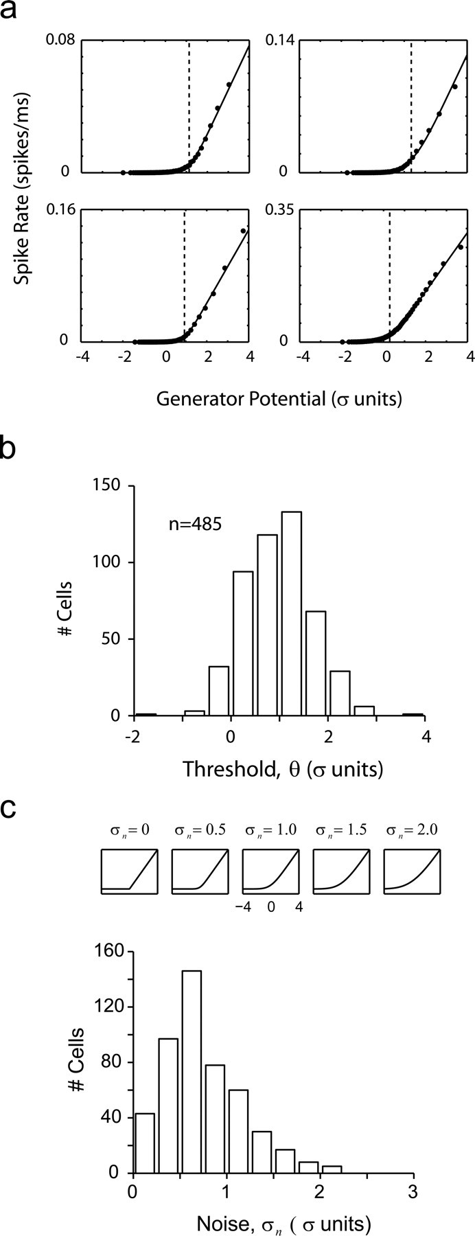
Reconstruction of nonlinearities in V1. a, Four examples showing the nonparametric estimates of the nonlinearities (filled data points) along with fits of the rectifier-plus-noise model (solid curves). It can be seen that the fits are excellent. b, Distribution of thresholds in V1 (at 99% contrast) shows that, on average, they cluster at ∼1 SD of the generator potential. c, The shape of nonlinearities in V1. The noise parameter σ_n controls the smoothness of the transition at the elbow of the nonlinearity. The distribution of fit values shows that, in general, transitions were relatively sharp.

It is worth emphasizing that the model assumes only temporal summation of stimulus responses. There are no assumptions made about spatial summation. Thus, in principle, the model can predict invariant responses to gratings of the same orientation and spatial frequency but different spatial phase. This allows both simple and complex cells to be considered on an equal footing in our formulation.

The model was tested by evaluating how well it can predict the responses to a novel sequence of frames (from the same stimulus set). The model performed well for both simple and complex cells (Fig. 4), achieving a correlation coefficient between the predicted and actual responses of 0.61 ± 0.12 SD.

Figure 4.

Example of the performance of the model in a simple cell (left) and in a complex cell (right). The top panels show the actual response of cells to a sequence of stimuli; the bottom panels show the predicted responses by the model.

Results

Nonlinearities are rectifiers with a threshold of ∼1 SD

We first investigated the shapes of the resulting nonlinearities in a large population of V1 cells at a high contrast level of 99% (n = 485). Four typical examples of the estimated nonlinearities are shown in Figure 5a. Here the filled dots represent the nonparametric estimates of the nonlinearity, and the solid curves are the fits from the model used in Figure 3d.

The distribution of thresholds was centered at 1 SD of the generator potential (0.96 ± 0.7 SD) (Fig. 5b). In other words, thresholds for spiking were, on average, ∼1 SD above the mean value of the generator potential; 1 SD represents the size of the minimum excursion that potentially could lead to a spike potential. As we note below, the average excursion leading to the generation of a spike is significantly larger.

The sharpness of the transition zone across the population can be studied by plotting the distribution of the parameter σ_n (Fig. 5c). The panels in the figure indicate the shape of the nonlinearities at various levels of σ_n, with the range of the x-axis set so that it is comparable to that of the generator signal. It can be seen that for these experiments, at high contrast, nonlinearities tend to have a sharp transition zone. Furthermore, it is worth noting that there is no significant saturation of the signal at high values of the generator potential; signals above the threshold appear to be amplified linearly.

These data indicate that the static nonlinearity can be considered as an ideal linear rectifier (with no saturation) and with a threshold near 1 SD of the generator signal.

Thresholds are relatively invariant to stimulus contrast

We repeated the experiment in a different population of neurons at lower contrast values ranging from 15 to 60% (n = 49 cells; average contrast of 35%). In this regimen of weaker stimulation we find that the thresholds of the estimated nonlinearities remain centered at ∼1 SD of the generator potential (compare Figs. 5b, 6a). There is no statistical difference between the means of thresholds at high and low contrasts (rank sum test; p > 0.7).

Figure 6.

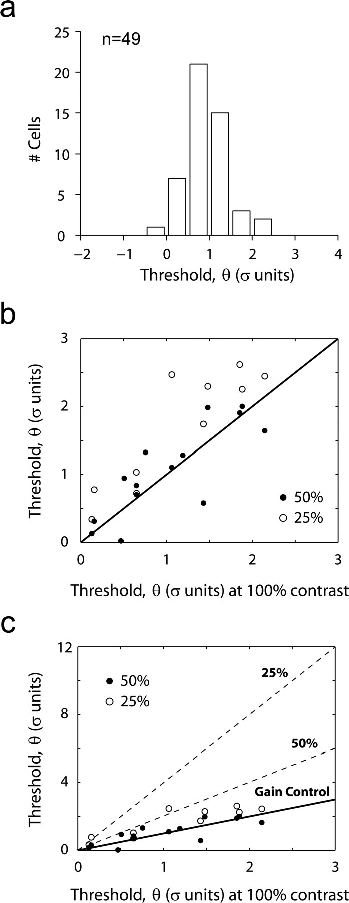
Thresholds are relatively invariant to contrast. a, Distribution of thresholds for low-contrast stimuli remain clustered at ∼1 SD (compare with Fig. 5b). A system without gain control would have predicted an overall shift of this distribution to higher thresholds. b, Thresholds at high and low contrast across a set of neurons. It can be seen that thresholds are invariant as contrast is reduced to 50% but show a tendency to increase at 25%. c, When the same data are plotted along with the predicted relationship in a system without gain control, however, it becomes apparent that compensation is nearly perfect for 25% contrast as well.

The significance of this result is understood best by considering the changes in threshold predicted in a system without gain control. Suppose that at a contrast of 100% we find that the threshold is θ̄. Decreasing the stimulus contrast by a factor α implies a decrease in the SD of the generator potential by the same factor (invoking the linearity of the front-end filter and the lack of gain control). This means that the threshold predicted at lower contrast increases by the same factor to αθ̄ (assuming that the properties of the spiking mechanism are not affected by the contrast of the stimulus).

Applying this reasoning to our data and considering that the mean threshold at 99% contrast was near 1 SD, the predicted thresholds for experiments with an average contrast of 35% would be distributed at ∼2.85. Clearly, this is not the case (Fig. 6a). Instead, the invariance of thresholds with changing contrast reflects gain control in this system: neuronal gain is increased to compensate for the decrease in contrast. Perfect compensation, in which gain is inversely proportional to contrast, predicts invariant thresholds.

To study this phenomenon in more detail, we performed the experiments at three contrasts levels (25, 50, and 99%) in the same population of cells (n = 14). The goal was to compare how threshold varies as a function of contrast in individual cells. A scatterplot of the thresholds at high contrasts (99%) versus those at 50% (filled symbols) and 25% (open symbols) is shown in Figure 6b. At 50% contrast there is a nearly complete invariance of thresholds, because the filled symbols lie very close to the unity line. The thresholds at 99 and 50% are not statistically different (paired signed rank test; p > 0.3). At the smaller contrast of 25% one can observe an overall trend for thresholds to be slightly higher (paired signed rank test; p < 0.002).

The magnitude of these changes can be placed in perspective by comparing these thresholds to those predicted in a linear system without gain control (Fig. 6c). The solid line represents the expected thresholds assuming perfect compensation by gain control (that is, invariant thresholds). The dashed lines represent the predicted thresholds in a system without gain control at levels of 50 and 25% contrast. The points corresponding to 25% contrast, although significantly above the unity line, are far from the dependence expected in a system with no gain control. Thus, gain control appears to compensate in large part for changes in contrast so that thresholds, in individual cells, remain relatively invariant over a significant range. The slight increase of thresholds at 25% is not surprising, because one would not want to invoke gain control when the signals are very small and noisy. As discussed below, the changes in gain in the front-end filter implied by our data are likely to be distributed across the early visual pathway and not restricted to the cortex.

We found no difference in threshold between simple and complex cells. Figure 7a shows the distribution of modulation indices ranging from 0 (complex) to 2 (simple) in our population. Thresholds showed no dependence with the rank-order of cells along the complex-simple dimension (Fig. 7b).

Figure 7.

Thresholds are independent of cell class. a, Distribution of the modulation ratio in our population of V1 cells. b, Threshold as a function of modulation index rank (with complex cells on the left and simple cells on the right). There is no obvious relationship between threshold and modulation index rank.

The operating point can sharpen neural selectivity

Thresholding has been claimed to increase the selectivity of spikes relative to that of the underlying membrane potential, a phenomenon referred to as the iceberg effect (Reid et al., 1987; Jagadeesh et al., 1993; Anderson et al., 2000b; Carandini and Ferster, 2000; Volgushev et al., 2000). It is therefore of interest to study how the selectivity of the generator potential, the predicted spike responses, and actual spike responses relate to each other in our data.

One way to quantify the overall degree of selectivity of a neuron with respect to a large stimulus space is by assessing the shape of the response distribution. A neuron that responds only to a small subset of stimuli will show a distribution with a mode at approximately zero (because the cell is silent most of the time) and a long tail. In contrast, a cell that responds to a broad range of stimuli may show a Gaussian distribution of responses. A statistic that naturally captures the differences in the shape of the response distributions is the kurtosis: high kurtosis results from distributions with peaks near zero and rare large deviations (heavy tails), whereas smaller values result from distributions with modest-sized deviations (Lehky and Sejnowski, 2004; Lehky et al., 2005; DeWeese and Zador, 2006). The kurtosis of a Gaussian variable has a value of 3, whereas distributions with high peaks near 0 and heavy tails have values >3.

When the kurtosis of the generator potential was analyzed, we found that it was highly non-Gaussian, with a mean kurtosis of 8.1 ± 7.1 SD (Fig. 8a). All of the data points had kurtosis larger than that expected from a Gaussian distribution (Fig. 8a, dashed line). As one would expect, the kurtosis of the generator potential correlates with the selectivity of the cell to the stimuli in the set, which we defined as the kurtosis of the stimulus-triggered responses (Fig. 3a) at the optimal time delay. Given that our stimuli span a region of the Fourier plane, the more selective the cell is in orientation and spatial frequency the higher the kurtosis of the associated generator potential (Fig. 8b). The kurtosis of the measured spike responses is clearly higher than that of the associated generator potential (Fig. 8c). The relationship between the kurtosis of the generator potential and the spike responses is explained by the static nonlinearity, because the predicted and measured kurtosis of spike responses match well (Fig. 8d). We can summarize these results by stating that the static nonlinearity served to increase the selectivity of spike responses relative to that of the generator potential.

Figure 8.

Neuronal selectivity and kurtosis of the generator potential. a, The distribution of the generator potential is highly non-Gaussian. The dashed line represents the kurtosis expected for a Gaussian distribution [log₁₀(3)]. All data points lie above this value. b, The kurtosis of the generator potential is, as expected, related to the selectivity of the cell to the stimulus set. c, The kurtosis of the spike responses is much higher than that of the generator potential. Thus, spike responses are more selective than is the generator potential. d, The increase in kurtosis in the spike responses can be explained by the nonlinear transformation between generator potential and spikes. The plot shows that the kurtosis predicted by the model matches very well that of the data.

We found that there is a simple descriptive model for the distribution of the generator potential across the population. To develop such a description, we investigated the relationship between the kurtosis and skewness of the generator potential across the population of cells (Fig. 9) (recall that the generator potential is normalized to have a zero mean and unit variance, so these moments are fixed). There is a strong covariation between these higher moments that is well approximated by assuming they conform to a gamma distribution with these parameters: $(a,1/\sqrt{a})$. This selection of parameters generates a distribution with unit variance and (kurtosis, skewness) values of $(3+6/a,2/\sqrt{a})$, which define the parametric solid curve in Figure 9. The small panels within Figure 8 show the shape of the distribution at various locations along this curve. It can be seen that at the bottom left corner, when kurtosis approaches values near 3, the distributions are close to Gaussian. As one moves toward the top right corner, the distributions become heavy-tailed and deviate strongly from Gaussian.

Figure 9.

The distribution of the generator potential is well approximated by a gamma distribution. This can be seen by plotting the relationship between the skewness and kurtosis of the generator potential (which already is normalized to have zero mean and unit variance). The resulting distribution can be approximated with a gamma distribution with parameters $(a,1/\sqrt{a})$, which describe the solid curve in the figure.

The finding that the distribution of the generator potential can be non-Gaussian also raises the question of whether the threshold is influenced by its kurtosis and skewness [instead of being controlled exclusively by the SD (Bonin et al., 2006)]. We found a positive (but weak) correlation between the threshold and both kurtosis (r = 0.28; p < 10⁻⁶) and skewness (r = 0.23; p < 10⁻⁶) (Fig. 10). Given the covariation between the skewness and kurtosis of the generator potential, the finding implies that thresholds tend to be higher the more the distribution departs from normality.

Figure 10.

Threshold dependence on kurtosis and skewness. Threshold is correlated positively with both kurtosis (a) and skewness (b). Although statistically significant, these correlations are weak.

The expected deviation of the generator potential causing a spike

The data indicate that thresholds for cortical V1 cells are 1 SD away from the mean of the generator potential. This means that significant positive excursions of the generator potential are needed for the cell to spike. How large are these signals expected to be? Note that signals that barely cross threshold are not very likely to yield a spike, because linear amplification above threshold implies a negligible rate of firing near threshold. At the other end, very large excursions above the mean are likely to produce a spike but are extremely unlikely to occur, given the distribution of the generator potential. What is the average size of the signal deviation that caused a spike in this model: E{z|spike}?

For the case of a rectifier without noise (σ_n = 0) and assuming a gamma distribution with parameters $(a,1/\sqrt{a})$, which provides a concise description of the empirical distributions (Fig. 9), this calculation yields the following:

Here, $\Gamma (a,z)={\displaystyle {\int }_z^{\infty }{{\displaystyle t}}^{a-1}{{\displaystyle e}}^{-t}dt}$ is the incomplete gamma function. The expected deviation causing a spike for various levels of the kurtosis and thresholds is shown in Figure 11a. The expected deviation increases with both the threshold and the kurtosis. The location of the plus sign in the figure corresponds to the coordinates of the mean values for the kurtosis and threshold in our population. At this location the mean deviation causing a spike is ∼2 SDs. Thus although the threshold is at 1 SD, on average a large deviation of twice the SD of the generator is needed to produce an output from the cell. This result is independent of the gain parameter, A. Note that, even for a Gaussian signal and a threshold of 1 SD, the expected deviation causing a spike is ∼1.57 SDs of the generator potential.

Figure 11.

Expected signal deviations causing a spike. a, The expected size of the excursion in the generator potential generating a spike is shown (in units of SD) as a function of both the threshold of the neuron and the kurtosis of the generator potential. For the mean values of the threshold and kurtosis the value is ∼2 SDs. b, Histogram of the expected deviation in our population of cells obtained by using the relationship in a while plugging in the estimated values of the threshold and kurtosis for each case. The distribution is centered near 2 SDs. Thus, despite thresholds being at 1 SD, on average the size of the generator potential excursion producing a spike is ∼2 SDs.

Using the above equation, we can compute the distribution of the expected deviations causing a spike in our population of cells by using the estimated values of threshold and kurtosis for each neuron. The resulting distribution has a mean of 1.9 ± 0.7 with a mode near 2 (Fig. 11b). Thus, in general, the mean excursion of the generator potential causing a spike is ∼2 SDs of the ongoing activity. This clarifies that the signal excursions generating a spike are, on average, rather large.

Lateral geniculate cells have thresholds near zero

Finally, one may ask whether the distribution of thresholds would necessarily be different if measured at earlier stages of visual processing. To investigate this possibility, we performed identical experiments in a number of lateral geniculate nucleus (LGN) cells (n = 20). These experiments were all done at a high contrast of 99%. Nonlinearities reconstructed in three cases are shown in Figure 12a. As in primary visual cortex the LGN nonlinearities are well approximated by a half-rectifier with noise (Eq. 2). However, in contrast to V1, the LGN nonlinearities had thresholds distributed near zero (Fig. 12b). The distribution of thresholds had a mean of −0.04 ± 0.36 SD and was significantly lower than that in V1 (Student's t test; p < 2 × 10⁻⁸). Thus the operating point of the LGN is very different from that of V1. Under the conditions of our experiments the geniculate cells appear simply to translate all excursions above the mean linearly, without a “dead zone.”

Figure 12.

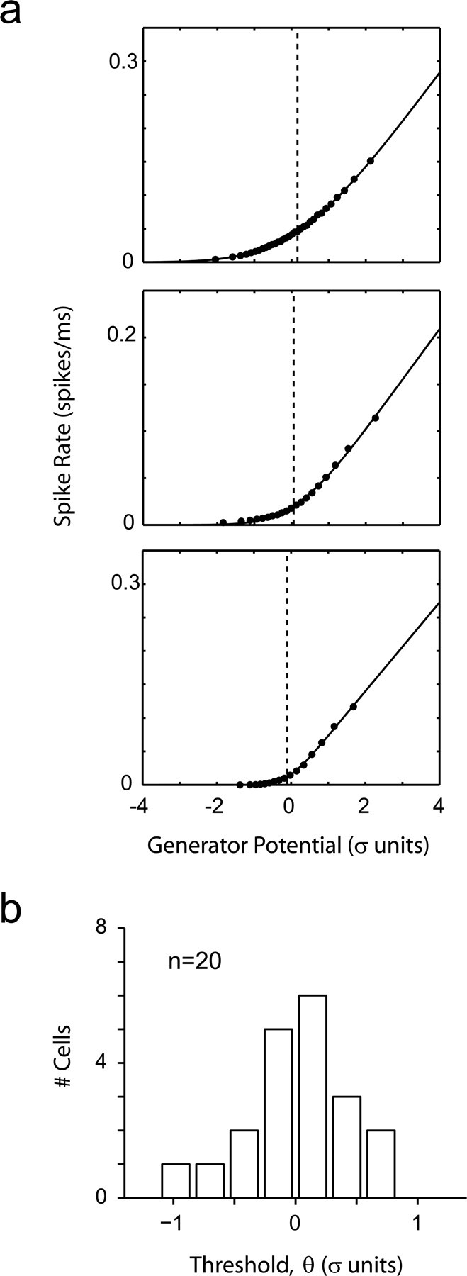
Thresholds in the LGN are very different from those in V1. a, Reconstructions of LGN nonlinearities. b, The distribution of thresholds in the LGN is centered at zero and is significantly different from the distribution of thresholds in V1.

The reconstruction of the LGN nonlinearities was performed with the same experimental protocol used in V1 cells. This demonstrates that in our experimental conditions there is not a strong saturation of the geniculate signal that could contribute to threshold invariance in V1 (Priebe and Ferster, 2006). Despite a nonsaturating LGN response, we cannot rule out that saturation of postsynaptic responses as recently described in cat visual cortex (Finn et al., 2007) contributes to the invariance of threshold with contrast.

Discussion

The shape of output nonlinearities

In this study we used a simple model of V1 neurons to study the operating point of cortical cells in primary visual cortex. We find that the spiking nonlinearities in LGN and V1 are well approximated by a half-rectifier with external noise (Anderson et al., 2000c; Hansel and van Vreeswijk, 2002; Miller and Troyer, 2002). The shape of our reconstructed nonlinearities, including the lack of significant saturation at high values of the generator signal, is in general agreement with similar estimates in the retina, LGN, and V1 (Chander and Chichilnisky, 2001; Kim and Rieke, 2001; Baccus and Meister, 2004; Carandini, 2004; Bonin et al., 2006; Sharpee et al., 2006). In one study Carandini (2004) fit a power law relationship between membrane voltage and spikes and found a mean exponent of 1.1 ± 0.6 across the population, which agrees well with the characterization of the nonlinearities as near-perfect half-rectifiers. In a previous study half-squaring was offered as a better descriptor (Anzai et al., 1999). This is likely a consequence of their methods estimating the shape of the nonlinearity near the transition zone, at relatively small contrasts.

Invariance of threshold to signal strength

Adaptation appears to keep the distance between the mean membrane potential and threshold for spiking at a constant distance for varying stimulus strengths. We arrive at this conclusion by observing the relative invariance of thresholds across the population at high and low contrasts (Figs. 5b, 6a) and even an invariance of thresholds within individual cells (Fig. 6c). This finding is consistent with the invariance of transmitted information under different stimulus conditions recently described in the barrel cortex (Maravall et al., 2007).

Control of normalized thresholds may result from changes in gain, resting membrane potential, or both (Carandini and Ferster, 1997; Sanchez-Vives et al., 2000a,b; Escabi et al., 2005). Intracellular measurements are needed to decide among these possibilities. Our results on gain control are similar to those observed in similar experiments in the retina and LGN (Shapley et al., 1972; Shapley and Victor, 1978; Benardete and Kaplan, 1999; Chander and Chichilnisky, 2001; Bonin et al., 2006). It is most likely that gain control in stages of processing preceding the cortex contribute to the overall gain captured by the lumped linear–nonlinear model.

The operating point of the cortex: neurons as large deviation detectors

We have seen that cortical cells rectify their inputs at a level of ∼1 SD of the on-going generator potential. Signals above threshold are translated linearly into spike rates, without reaching saturation. Furthermore, the non-Gaussian distribution of the generator potential and spike thresholding combine so that the expected deviation causing a spike is ∼2 SDs of the generator signal. Thus the operating point of the cortex is such that cells behave as “large-deviation detectors.”

Previous studies have suggested that adaptive mechanisms work primarily to maximize the faithful transmission of information, given the statistics of the underlying signal (Laughlin, 1981; Smirnakis et al., 1997; van Hateren, 1997; Brenner et al., 2000). In the LGN, where we have shown that thresholds are near zero and two populations of cells (ON/OFF) are known to code for the sign of the fluctuations, these ideas may be applicable. Our findings indicate that in the cortex, however, this cannot be the case. Clearly, by clipping the signals below a threshold of ∼1 SD, information about the generator signal obviously is being lost (Yu et al., 2005). Instead, neurons are better described as detecting and amplifying large signals that may be of potential interest while rejecting background noise (Poor and Thomas, 1979; Moustakides, 1985; Yang et al., 2004; Abramovich et al., 2006).

It is tempting to speculate that a steady increase in normalized thresholds would be seen at higher levels in the visual hierarchy, similar to the relationship that holds between the LGN and V1. This may explain the remarkable finding that some cells in high visual areas of human cortex show surprisingly high sparseness and selectivity (Quiroga et al., 2005; Waydo et al., 2006). A similar increase in thresholds at successive levels of the processing stream recently has been described in the olfactory system of the locust, where it generates high selectivity and sparseness in Kenyon cells (Jortner et al., 2007).

Neuronal selectivity

The distribution of the generator potential when cells are stimulated by a rapid sequence of gratings of varying orientations and spatial frequencies has a heavy tail and is well approximated by a gamma distribution. The kurtosis of the generator potential reflects the selectivity of neurons for the stimulus set [Lehky et al. (2005) refer to this measure as nonparametric selectivity]. We find that, as expected, selectivity is enhanced by the static nonlinearity such that selectivity and sparseness of the spike responses are increased (Fig. 7). The relatively high thresholds observed in V1 certainly would serve to enhance the selectivity of the subthreshold signals (Reid et al., 1987; Jagadeesh et al., 1993; Anderson et al., 2000b; Carandini and Ferster, 2000; Volgushev et al., 2000; Pena and Konishi, 2002; Escabi et al., 2005).

The view of gain control and thresholding in establishing the operating point of the cortex is consistent with some previous studies. In particular, it has been found that the selectivity and sparseness of individual neurons increase with the size of the stimulation area beyond the classical receptive field of the cell (Vinje and Gallant, 2000, 2002). As the stimulus is increased, it is expected that gain would decrease (Cavanaugh et al., 2002a,b), implying an increase in normalized threshold that could induce a corresponding decrease in firing rate while increasing response selectivity and sparseness.

Our findings are also in agreement with a study of the responses of neurons in the inferior colliculus to auditory stimuli (Escabi et al., 2005). Escabi and colleagues (2005) described an inverse relationship between thresholding and selectivity in their population of cells. They found that neurons with the highest thresholds reliably signaled the occurrence of specific stimulus features of the acoustic signal. However, these were the cells with the lowest amount of total transmitted information. Neurons with lower thresholds had higher total information rates but lower selectivity. A simple thresholding model was successful in accounting for these dependencies.

The high kurtosis of the membrane potential inferred from our experiments is mostly a consequence of the stimulus set used and does not necessarily conflict with previous studies that have observed a Gaussian distribution under different stimulation conditions (Ferster and Jagadeesh, 1992; Carandini, 2004). It is also possible that the modulation of up/down states by visual stimulation is involved in the generation of a non-Gaussian distribution of the generator potential (Anderson et al., 2000a). One could potentially incorporate a hidden binary variable representing the state of the cell to model such a system (Paninski, 2006). It is also worth noting that a recent study in auditory cortex found non-Gaussian distributions of membrane potential resembling the ones we infer by fitting the linear–nonlinear model (DeWeese and Zador, 2006).

Implications for cortical processing

The distribution of normalized thresholds in V1 neurons implies that reliable information transmission is not the central goal of cortical processing. This may not be entirely surprising. After all, at some point in the visual hierarchy one would expect the brain to start processing the signals instead of merely transmitting them. Even when the front-end spatiotemporal filters of some neurons are linear, like those of simple cells (Movshon et al., 1978), the operating point would suggest that neurons behave more as “matched filter” detectors rather than straightforward linear filters (De Valois et al., 1979). In other words, the front-end linear filter endows the generator potential with broad tuning, whereas the operating point ensures that only stimuli that closely match the front-end filter generate a spiking response by the neuron.

The data may be consistent with the idea that the cortical network works to generate a sparse representation of the image (Olshausen and Field, 1996, 2000; Simoncelli and Olshausen, 2001). Controlling the sparseness across a population of cells could be achieved by having the same population participate in the gain control pool (Carandini et al., 1997; Chance et al., 2002).

The thresholding of the generator potential may serve to generate a de-noised version of the retinal image by a procedure analogous to “wavelet shrinkage” (Donoho and Johnstone, 1994, 1995; Donoho et al., 1995; Chang et al., 2000a,b; Jung and Scharcanski, 2003; Bacchelli and Papi, 2004; Abramovich et al., 2006). Thus a broad hypothesis about V1 processing is that it serves to create a sparse representation of a de-noised version of the image by dynamically adjusting the operating point by adapting to the statistics of the input.

Limitations of the study

In interpreting these results one should keep in mind some limitations of the study. First, in the simple linear–nonlinear model the generator potential represents an underlying variable that conveys information about the instantaneous probability of spiking. One should be careful not to assume that the generator potential has a direct biophysical interpretation, such as representing the membrane potential of the cell, membrane conductance, or synaptic currents. Indeed, both experimental and theoretical studies suggests that the generator potential is better understood as representing a combination of the history of intracellular variables that results in an single measure overall of neuronal drive (Lankheet et al., 1989; Anderson et al., 2000b; Aguera y Arcas and Fairhall, 2003; Aguera y Arcas et al., 2003).

Second, gain control in the model works by scaling the output of a lumped linear filter representing all previous processing up to the input of the static nonlinearity. It should not be assumed that the gain control changes implied by our data occur exclusively at the cortical level. In fact, there is reason to believe that gain changes are distributed across the early visual pathway, including the retina, the LGN, and cortex (Shapley and Victor, 1979; Smirnakis et al., 1997; Chander and Chichilnisky, 2001; Carandini et al., 2002; Demb, 2002; Freeman et al., 2002; Solomon et al., 2004; Bonin et al., 2006).

Finally, we must consider that the operating point of the cortex may be susceptible to the level of anesthesia and, furthermore, that such effects may be different between the LGN and cortex (Steriade et al., 1993; Steriade et al., 2001; Destexhe et al., 2007; Haider et al., 2007). We observed no statistically significant differences between these data and a smaller subset obtained by using a combination of sufentanil and midazolam (Ringach, 2002). This includes the overall distribution of spontaneous firing rates, peak firing rates during visual stimulation, and estimates of the effective threshold. Thus we do not think the anesthetic plane with propofol was one in which the cortex was severely depressed, leading to estimates of artificially high thresholds. In addition, the distributions of spontaneous activity and orientation selectivity in our data and those in alert V1 are similar to each other (Gur et al., 2005). Nevertheless, analogous experiments in awake, behaving animals may be necessary to verify that our results hold in general.

References

- Abramovich F, Benjamini Y, Donoho DL, Johnstone IM. Adapting to unknown sparsity by controlling the false discovery rate. Ann Stat. 2006;34:584–653. [Google Scholar]
- Aguera y Arcas B, Fairhall AL. What causes a neuron to spike? Neural Comput. 2003;15:1789–1807. doi: 10.1162/08997660360675044. [DOI] [PubMed] [Google Scholar]
- Aguera y Arcas B, Fairhall AL, Bialek W. Computation in a single neuron: Hodgkin and Huxley revisited. Neural Comput. 2003;15:1715–1749. doi: 10.1162/08997660360675017. [DOI] [PubMed] [Google Scholar]
- Anderson JS, Lampl I, Reichova I, Carandini M, Ferster D. Stimulus dependence of two-state fluctuations of membrane potential in cat visual cortex. Nat Neurosci. 2000a;3:617–621. doi: 10.1038/75797. [DOI] [PubMed] [Google Scholar]
- Anderson JS, Carandini M, Ferster D. Orientation tuning of input conductance, excitation, and inhibition in cat primary visual cortex. J Neurophysiol. 2000b;84:909–926. doi: 10.1152/jn.2000.84.2.909. [DOI] [PubMed] [Google Scholar]
- Anderson JS, Lampl I, Gillespie DC, Ferster D. The contribution of noise to contrast invariance of orientation tuning in cat visual cortex. Science. 2000c;290:1968–1972. doi: 10.1126/science.290.5498.1968. [DOI] [PubMed] [Google Scholar]
- Anzai A, Ohzawa I, Freeman RD. Neural mechanisms for processing binocular information I. Simple cells. J Neurophysiol. 1999;82:891–908. doi: 10.1152/jn.1999.82.2.891. [DOI] [PubMed] [Google Scholar]
- Atick JJ. Could information theory provide an ecological theory of sensory processing? Network: Comput Neural Syst. 1992;3:213–251. doi: 10.3109/0954898X.2011.638888. [DOI] [PubMed] [Google Scholar]
- Bacchelli S, Papi S. Filtered wavelet thresholding methods. J Comput Appl Math. 2004;164–165:39–52. [Google Scholar]
- Baccus SA, Meister M. Retina versus cortex: contrast adaptation in parallel visual pathways. Neuron. 2004;42:5–7. doi: 10.1016/s0896-6273(04)00187-4. [DOI] [PubMed] [Google Scholar]
- Baddeley R, Abbott LF, Booth MCA, Sengpiel F, Freeman T, Wakeman EA, Rolls ET. Responses of neurons in primary and inferior temporal visual cortices to natural scenes. Proc R Soc Lond B Biol Sci. 1997;264:1775–1783. doi: 10.1098/rspb.1997.0246. [DOI] [PMC free article] [PubMed] [Google Scholar]
- Benardete EA, Kaplan E. The dynamics of primate M retinal ganglion cells. Vis Neurosci. 1999;16:355–368. doi: 10.1017/s0952523899162151. [DOI] [PubMed] [Google Scholar]
- Bonin V, Mante V, Carandini M. The statistical computation underlying contrast gain control. J Neurosci. 2006;26:6346–6353. doi: 10.1523/JNEUROSCI.0284-06.2006. [DOI] [PMC free article] [PubMed] [Google Scholar]
- Brenner N, Bialek W, de Ruyter van Steveninck R. Adaptive rescaling maximizes information transmission. Neuron. 2000;26:695–702. doi: 10.1016/s0896-6273(00)81205-2. [DOI] [PubMed] [Google Scholar]
- Carandini M. Amplification of trial-to-trial response variability by neurons in visual cortex. PLoS Biol. 2004;2:1483–1493. doi: 10.1371/journal.pbio.0020264. [DOI] [PMC free article] [PubMed] [Google Scholar]
- Carandini M, Ferster D. A tonic hyperpolarization underlying contrast adaptation in cat visual cortex. Science. 1997;276:949–952. doi: 10.1126/science.276.5314.949. [DOI] [PubMed] [Google Scholar]
- Carandini M, Ferster D. Membrane potential and firing rate in cat primary visual cortex. J Neurosci. 2000;20:470–484. doi: 10.1523/JNEUROSCI.20-01-00470.2000. [DOI] [PMC free article] [PubMed] [Google Scholar]
- Carandini M, Heeger DJ, Movshon JA. Linearity and normalization in simple cells of the macaque primary visual cortex. J Neurosci. 1997;17:8621–8644. doi: 10.1523/JNEUROSCI.17-21-08621.1997. [DOI] [PMC free article] [PubMed] [Google Scholar]
- Carandini M, Heeger DJ, Senn W. A synaptic explanation of suppression in visual cortex. J Neurosci. 2002;22:10053–10065. doi: 10.1523/JNEUROSCI.22-22-10053.2002. [DOI] [PMC free article] [PubMed] [Google Scholar]
- Cavanaugh JR, Bair W, Movshon JA. Nature and interaction of signals from the receptive field center and surround in macaque V1 neurons. J Neurophysiol. 2002a;88:2530–2546. doi: 10.1152/jn.00692.2001. [DOI] [PubMed] [Google Scholar]
- Cavanaugh JR, Bair W, Movshon JA. Selectivity and spatial distribution of signals from the receptive field surround in macaque V1 neurons. J Neurophysiol. 2002b;88:2547–2556. doi: 10.1152/jn.00693.2001. [DOI] [PubMed] [Google Scholar]
- Chance FS, Abbott LF, Reyes AD. Gain modulation from background synaptic input. Neuron. 2002;35:773–782. doi: 10.1016/s0896-6273(02)00820-6. [DOI] [PubMed] [Google Scholar]
- Chander D, Chichilnisky EJ. Adaptation to temporal contrast in primate and salamander retina. J Neurosci. 2001;21:9904–9916. doi: 10.1523/JNEUROSCI.21-24-09904.2001. [DOI] [PMC free article] [PubMed] [Google Scholar]
- Chang SG, Yu B, Vetterli M. Spatially adaptive wavelet thresholding with context modeling for image denoising. IEEE Trans Image Process. 2000a;9:1522–1531. doi: 10.1109/83.862630. [DOI] [PubMed] [Google Scholar]
- Chang SG, Yu B, Vetterli M. Adaptive wavelet thresholding for image denoising and compression. IEEE Trans Image Process. 2000b;9:1532–1546. doi: 10.1109/83.862633. [DOI] [PubMed] [Google Scholar]
- Chichilnisky EJ. A simple white noise analysis of neuronal light responses. Network. 2001;12:199–213. [PubMed] [Google Scholar]
- Deangelis GC, Ohzawa I, Freeman RD. Spatiotemporal organization of simple-cell receptive-fields in the cats striate cortex. 2. Linearity of temporal and spatial summation. J Neurophysiol. 1993;69:1118–1135. doi: 10.1152/jn.1993.69.4.1118. [DOI] [PubMed] [Google Scholar]
- Deboer E, Kuyper P. Triggered correlation. IEEE Trans Biomed Eng. 1968;15:169–179. doi: 10.1109/tbme.1968.4502561. [DOI] [PubMed] [Google Scholar]
- Demb JB. Multiple mechanisms for contrast adaptation in the retina. Neuron. 2002;36:781–783. doi: 10.1016/s0896-6273(02)01100-5. [DOI] [PubMed] [Google Scholar]
- Destexhe A, Hughes SW, Rudolph M, Crunelli V. Are corticothalamic “up” states fragments of wakefulness? Trends Neurosci. 2007 doi: 10.1016/j.tins.2007.04.006. in press. [DOI] [PMC free article] [PubMed] [Google Scholar]
- De Valois KK, De Valois RL, Yund EW. Responses of striate cortex cells to grating and checkerboard patterns. J Physiol (Lond) 1979;291:483–505. doi: 10.1113/jphysiol.1979.sp012827. [DOI] [PMC free article] [PubMed] [Google Scholar]
- Deweese M. Optimization principles for the neural code*. Network. 1996;7:325–331. doi: 10.1088/0954-898X/7/2/013. [DOI] [PubMed] [Google Scholar]
- DeWeese MR, Zador AM. Non-Gaussian membrane potential dynamics imply sparse, synchronous activity in auditory cortex. J Neurosci. 2006;26:12206–12218. doi: 10.1523/JNEUROSCI.2813-06.2006. [DOI] [PMC free article] [PubMed] [Google Scholar]
- Donoho DL, Johnstone IM. Ideal spatial adaptation by wavelet shrinkage. Biometrika. 1994;81:425–455. [Google Scholar]
- Donoho DL, Johnstone IM. Adapting to unknown smoothness via wavelet shrinkage. J Am Stat Assn. 1995;90:1200–1224. [Google Scholar]
- Donoho DL, Johnstone IM, Kerkyacharian G, Picard D. Wavelet shrinkage: asymptopia. J R Stat Soc Ser B. 1995;57:301–337. [Google Scholar]
- Escabi MA, Nassiri R, Miller LM, Schreiner CE, Read HL. The contribution of spike threshold to acoustic feature selectivity, spike information content, and information throughput. J Neurosci. 2005;25:9524–9534. doi: 10.1523/JNEUROSCI.1804-05.2005. [DOI] [PMC free article] [PubMed] [Google Scholar]
- Fairhall AL, Lewen GD, Bialek W, de Ruyter Van Steveninck RR. Efficiency and ambiguity in an adaptive neural code. Nature. 2001;412:787–792. doi: 10.1038/35090500. [DOI] [PubMed] [Google Scholar]
- Ferster D, Jagadeesh B. EPSP–IPSP interactions in cat visual cortex studied with in vivo whole-cell patch recording. J Neurosci. 1992;12:1262–1274. doi: 10.1523/JNEUROSCI.12-04-01262.1992. [DOI] [PMC free article] [PubMed] [Google Scholar]
- Finn IM, Priebe NJ, Ferster D. The emergence of contrast-invariant orientation tuning in simple cells of cat visual cortex. Neuron. 2007;54:137–152. doi: 10.1016/j.neuron.2007.02.029. [DOI] [PMC free article] [PubMed] [Google Scholar]
- Freeman TCB, Durand S, Kiper DC, Carandini M. Suppression without inhibition in visual cortex. Neuron. 2002;35:759–771. doi: 10.1016/s0896-6273(02)00819-x. [DOI] [PubMed] [Google Scholar]
- Granit R, Shortess GK, Kernell D. Quantitative aspects of repetitive firing of mammalian motoneurones, caused by injected currents. J Physiol (Lond) 1963;168:911–931. doi: 10.1113/jphysiol.1963.sp007230. [DOI] [PMC free article] [PubMed] [Google Scholar]
- Gur M, Kagan I, Snodderly DM. Orientation and direction selectivity of neurons in V1 of alert monkeys: functional relationships and laminar distributions. Cereb Cortex. 2005;15:1207–1221. doi: 10.1093/cercor/bhi003. [DOI] [PubMed] [Google Scholar]
- Haider B, Duque A, Hasenstaub AR, Yu Y, McCormick DA. Enhancement of visual responsiveness by spontaneous local network activity in vivo. J Neurophysiol. 2007;97:4186–4202. doi: 10.1152/jn.01114.2006. [DOI] [PubMed] [Google Scholar]
- Hansel D, van Vreeswijk C. How noise contributes to contrast invariance of orientation tuning in cat visual cortex. J Neurosci. 2002;22:5118–5128. doi: 10.1523/JNEUROSCI.22-12-05118.2002. [DOI] [PMC free article] [PubMed] [Google Scholar]
- Heeger DJ. Normalization of cell responses in cat striate cortex. Vis Neurosci. 1992;9:181–197. doi: 10.1017/s0952523800009640. [DOI] [PubMed] [Google Scholar]
- Hunter IW, Korenberg MJ. The identification of nonlinear biological systems: Wiener and Hammerstein cascade models. Biol Cybern. 1986;55:135–144. doi: 10.1007/BF00341929. [DOI] [PubMed] [Google Scholar]
- Jagadeesh B, Wheat HS, Ferster D. Linearity of summation of synaptic potentials underlying direction selectivity in simple cells of the cat visual cortex. Science. 1993;262:1901–1904. doi: 10.1126/science.8266083. [DOI] [PubMed] [Google Scholar]
- Jones JP, Palmer LA. An evaluation of the two-dimensional Gabor filter model of simple receptive fields in cat striate cortex. J Neurophysiol. 1987;58:1233–1258. doi: 10.1152/jn.1987.58.6.1233. [DOI] [PubMed] [Google Scholar]
- Jortner RA, Farivar SS, Laurent G. A simple connectivity scheme for sparse coding in an olfactory system. J Neurosci. 2007;27:1659–1669. doi: 10.1523/JNEUROSCI.4171-06.2007. [DOI] [PMC free article] [PubMed] [Google Scholar]
- Jung CR, Scharcanski J. Adaptive image denoising and edge enhancement in scale-space using the wavelet transform. Pattern Recognit Lett J. 2003;24:965–971. [Google Scholar]
- Kim KJ, Rieke F. Temporal contrast adaptation in the input and output signals of salamander retinal ganglion cells. J Neurosci. 2001;21:287–299. doi: 10.1523/JNEUROSCI.21-01-00287.2001. [DOI] [PMC free article] [PubMed] [Google Scholar]
- Lankheet MJ, Molenaar J, van de Grind WA. The spike generating mechanism of cat retinal ganglion cells. Vision Res. 1989;29:505–517. doi: 10.1016/0042-6989(89)90037-0. [DOI] [PubMed] [Google Scholar]
- Laughlin S. A simple coding procedure enhances a neuron's information capacity. Z Naturforsch [C] 1981;36:910–912. [PubMed] [Google Scholar]
- Lehky S, Sejnowski T. Selectivity and ergodicity in striate complex cells. Perception. 2004;33:67. [Google Scholar]
- Lehky SR, Sejnowski TJ, Desimone R. Selectivity and sparseness in the responses of striate complex cells. Vision Res. 2005;45:57–73. doi: 10.1016/j.visres.2004.07.021. [DOI] [PMC free article] [PubMed] [Google Scholar]
- Maravall M, Petersen RS, Fairhall AL, Arabzadeh E, Diamond ME. Shifts in coding properties and maintenance of information transmission during adaptation in barrel cortex. PLoS Biol. 2007 doi: 10.1371/journal.pbio.0050019. in press. [DOI] [PMC free article] [PubMed] [Google Scholar]
- Miller KD, Troyer TW. Neural noise can explain expansive, power-law nonlinearities in neural response functions. J Neurophysiol. 2002;87:653–659. doi: 10.1152/jn.00425.2001. [DOI] [PubMed] [Google Scholar]
- Moustakides GV. Robust detection of signals: a large deviations approach. IEEE Trans Inf Theory. 1985;31:822–825. [Google Scholar]
- Movshon JA, Thompson ID, Tolhurst DJ. Spatial summation in receptive fields of simple cells in cats striate cortex. J Physiol (Lond) 1978;283:53–77. doi: 10.1113/jphysiol.1978.sp012488. [DOI] [PMC free article] [PubMed] [Google Scholar]
- Nagel KI, Doupe AJ. Temporal processing and adaptation in the songbird auditory forebrain. Neuron. 2006;51:845–859. doi: 10.1016/j.neuron.2006.08.030. [DOI] [PubMed] [Google Scholar]
- Nishimoto S, Arai M, Ohzawa I. Accuracy of subspace mapping of spatiotemporal frequency domain visual receptive fields. J Neurophysiol. 2005;93:3524–3536. doi: 10.1152/jn.01169.2004. [DOI] [PubMed] [Google Scholar]
- Nykamp DQ, Ringach DL. Full identification of a linear–nonlinear system via cross-correlation analysis. J Vis. 2002;2:1–11. doi: 10.1167/2.1.1. [DOI] [PubMed] [Google Scholar]
- Ohzawa I, Sclar G, Freeman RD. Contrast gain control in the cat visual cortex. Nature. 1982;298:266–268. doi: 10.1038/298266a0. [DOI] [PubMed] [Google Scholar]
- Olshausen BA, Field DJ. Natural image statistics and efficient coding. Network. 1996;7:333–339. doi: 10.1088/0954-898X/7/2/014. [DOI] [PubMed] [Google Scholar]
- Olshausen BA, Field DJ. Vision and the coding of natural images. Am Sci. 2000;88:238–245. [Google Scholar]
- Paninski L. The spike-triggered average of the integrate-and-fire cell driven by Gaussian white noise. Neural Comput. 2006;18:2592–2616. doi: 10.1162/neco.2006.18.11.2592. [DOI] [PubMed] [Google Scholar]
- Pena JL, Konishi M. From postsynaptic potentials to spikes in the genesis of auditory spatial receptive fields. J Neurosci. 2002;22:5652–5658. doi: 10.1523/JNEUROSCI.22-13-05652.2002. [DOI] [PMC free article] [PubMed] [Google Scholar]
- Poor HV, Thomas JB. Memoryless discrete-time detection of a constant signal in M-dependent noise. IEEE Trans Inf Theory. 1979;25:54–61. [Google Scholar]
- Priebe NJ, Ferster D. Mechanisms underlying cross-orientation suppression in cat visual cortex. Nat Neurosci. 2006;9:552–561. doi: 10.1038/nn1660. [DOI] [PubMed] [Google Scholar]
- Quiroga RQ, Reddy L, Kreiman G, Koch C, Fried I. Invariant visual representation by single neurons in the human brain. Nature. 2005;435:1102–1107. doi: 10.1038/nature03687. [DOI] [PubMed] [Google Scholar]
- Reid RC, Soodak RE, Shapley RM. Linear mechanisms of directional selectivity in simple cells of cat striate cortex. Proc Natl Acad Sci USA. 1987;84:8740–8744. doi: 10.1073/pnas.84.23.8740. [DOI] [PMC free article] [PubMed] [Google Scholar]
- Reid RC, Victor JD, Shapley RM. The use of M-sequences in the analysis of visual neurons: linear receptive field properties. Vis Neurosci. 1997;14:1015–1027. doi: 10.1017/s0952523800011743. [DOI] [PubMed] [Google Scholar]
- Ringach DL. Spatial structure and symmetry of simple-cell receptive fields in macaque primary visual cortex. J Neurophysiol. 2002;88:455–463. doi: 10.1152/jn.2002.88.1.455. [DOI] [PubMed] [Google Scholar]
- Sanchez-Vives MV, Nowak LG, McCormick DA. Membrane mechanisms underlying contrast adaptation in cat area 17 in vivo. J Neurosci. 2000a;20:4267–4285. doi: 10.1523/JNEUROSCI.20-11-04267.2000. [DOI] [PMC free article] [PubMed] [Google Scholar]
- Sanchez-Vives MV, Nowak LG, McCormick DA. Cellular mechanisms of long-lasting adaptation in visual cortical neurons in vitro. J Neurosci. 2000b;20:4286–4299. doi: 10.1523/JNEUROSCI.20-11-04286.2000. [DOI] [PMC free article] [PubMed] [Google Scholar]
- Sclar G, Ohzawa I, Freeman RD. Contrast gain control in the kitten's visual system. J Neurophysiol. 1985;54:668–675. doi: 10.1152/jn.1985.54.3.668. [DOI] [PubMed] [Google Scholar]
- Shapley RM, Victor JD. The effect of contrast on the transfer properties of cat retinal ganglion cells. J Physiol (Lond) 1978;285:275–298. doi: 10.1113/jphysiol.1978.sp012571. [DOI] [PMC free article] [PubMed] [Google Scholar]
- Shapley RM, Victor JD. The contrast gain control of the cat retina. Vision Res. 1979;19:431–434. doi: 10.1016/0042-6989(79)90109-3. [DOI] [PubMed] [Google Scholar]
- Shapley RM, Enroth-Cugell C, Bonds AB, Kirby A. Gain control in retina and retinal dynamics. Nature. 1972;236:352–353. doi: 10.1038/236352a0. [DOI] [PubMed] [Google Scholar]
- Sharpee TO, Sugihara H, Kurgansky AV, Rebrik SP, Stryker MP, Miller KD. Adaptive filtering enhances information transmission in visual cortex. Nature. 2006;439:936–942. doi: 10.1038/nature04519. [DOI] [PMC free article] [PubMed] [Google Scholar]
- Simoncelli EP, Olshausen BA. Natural image statistics and neural representation. Annu Rev Neurosci. 2001;24:1193–1216. doi: 10.1146/annurev.neuro.24.1.1193. [DOI] [PubMed] [Google Scholar]
- Skottun BC, De Valois RL, Grosof DH, Movshon JA, Albrecht DG, Bonds AB. Classifying simple and complex cells on the basis of response modulation. Vision Res. 1991;31:1079–1086. doi: 10.1016/0042-6989(91)90033-2. [DOI] [PubMed] [Google Scholar]
- Smirnakis SM, Berry MJ, Warland DK, Bialek W, Meister M. Adaptation of retinal processing to image contrast and spatial scale. Nature. 1997;386:69–73. doi: 10.1038/386069a0. [DOI] [PubMed] [Google Scholar]
- Solomon SG, Peirce JW, Dhruv NT, Lennie P. Profound contrast adaptation early in the visual pathway. Neuron. 2004;42:155–162. doi: 10.1016/s0896-6273(04)00178-3. [DOI] [PubMed] [Google Scholar]
- Steriade M, McCormick DA, Sejnowski TJ. Thalamocortical oscillations in the sleeping and aroused brain. Science. 1993;262:679–685. doi: 10.1126/science.8235588. [DOI] [PubMed] [Google Scholar]
- Steriade M, Timofeev I, Grenier F. Natural waking and sleep states: a view from inside neocortical neurons. J Neurophysiol. 2001;85:1969–1985. doi: 10.1152/jn.2001.85.5.1969. [DOI] [PubMed] [Google Scholar]
- Truchard AM, Ohzawa I, Freeman RD. Contrast gain control in the visual cortex: monocular versus binocular mechanisms. J Neurosci. 2000;20:3017–3032. doi: 10.1523/JNEUROSCI.20-08-03017.2000. [DOI] [PMC free article] [PubMed] [Google Scholar]
- van Hateren JH. A theory of maximizing sensory information. Biol Cybern. 1992;68:23–29. doi: 10.1007/BF00203134. [DOI] [PubMed] [Google Scholar]
- van Hateren JH. Processing of natural time series of intensities by the visual system of the blowfly. Vision Res. 1997;37:3407–3416. doi: 10.1016/s0042-6989(97)00105-3. [DOI] [PubMed] [Google Scholar]
- Vinje WE, Gallant JL. Sparse coding and decorrelation in primary visual cortex during natural vision. Science. 2000;287:1273–1276. doi: 10.1126/science.287.5456.1273. [DOI] [PubMed] [Google Scholar]
- Vinje WE, Gallant JL. Natural stimulation of the nonclassical receptive field increases information transmission efficiency in V1. J Neurosci. 2002;22:2904–2915. doi: 10.1523/JNEUROSCI.22-07-02904.2002. [DOI] [PMC free article] [PubMed] [Google Scholar]
- Volgushev M, Pernberg J, Eysel UT. Comparison of the selectivity of postsynaptic potentials and spike responses in cat visual cortex. Eur J Neurosci. 2000;12:257–263. doi: 10.1046/j.1460-9568.2000.00909.x. [DOI] [PubMed] [Google Scholar]
- von der Twer T, MacLeod DI. Optimal nonlinear codes for the perception of natural colours. Network. 2001;12:395–407. [PubMed] [Google Scholar]
- Wainwright MJ. Visual adaptation as optimal information transmission. Vision Res. 1999;39:3960–3974. doi: 10.1016/s0042-6989(99)00101-7. [DOI] [PubMed] [Google Scholar]
- Waydo S, Kraskov A, Quiroga RQ, Fried I, Koch C. Sparse representation in the human medial temporal lobe. J Neurosci. 2006;26:10232–10234. doi: 10.1523/JNEUROSCI.2101-06.2006. [DOI] [PMC free article] [PubMed] [Google Scholar]
- Yang XS, Poor HV, Petropulu AP. Memoryless discrete-time signal detection in long-range dependent noise. IEEE Trans Signal Process. 2004;52:1607–1619. [Google Scholar]
- Yu YG, Potetz B, Lee TS. The role of spiking nonlinearity in contrast gain control and information transmission. Vision Res. 2005;45:583–592. doi: 10.1016/j.visres.2004.09.024. [DOI] [PubMed] [Google Scholar]