Functional Imaging of Primary Visual Cortex Using Flavoprotein Autofluorescence

Abstract

Neuronal autofluorescence, which results from the oxidation of flavoproteins in the electron transport chain, has recently been used to map cortical responses to sensory stimuli. This approach could represent a substantial improvement over other optical imaging methods because it is a direct (i.e., nonhemodynamic) measure of neuronal metabolism. However, its application to functional imaging has been limited because strong responses have been reported only in rodents. In this study, we demonstrate that autofluorescence imaging (AFI) can be used to map the functional organization of primary visual cortex in both mouse and cat. In cat area 17, orientation preference maps generated by AFI had the classic pinwheel structure and matched those generated by intrinsic signal imaging in the same imaged field. The spatiotemporal profile of the autofluorescence signal had several advantages over intrinsic signal imaging, including spatially restricted fluorescence throughout its response duration, reduced susceptibility to vascular artifacts, an improved spatial response profile, and a faster time course. These results indicate that AFI is a robust and useful measure of large-scale cortical activity patterns in visual mammals.

Introduction

The functional organization of neocortex has been heavily studied using a variety of optical imaging techniques, each relying on a different kind of abstraction of neural activity. The most commonly used technique, intrinsic signal imaging (ISI), relies on local blood oxygenation changes with the assumption that oxygenation is inversely related to the metabolic demands of active neurons (for review, see Bonhoeffer and Grinvald, 1996). Although ISI has provided high-resolution maps of several cortical features, it suffers from limitations that can hamper the interpretation of response patterns. Most of these artifacts arise because the most significant component of the signal is produced by hemoglobin, and is therefore tightly coupled to vascular structure and dynamics (Frostig et al., 1990; Ts'o et al., 1990; Malonek and Grinvald, 1996; Malonek et al., 1997; Cannestra et al., 1998; Harrison et al., 2002). In particular, fluctuations in vascular light absorbance, either independent of neuronal activity or driven by a stimulus, create the potential for misclassifying activity patterns around vessels.

Flavoprotein autofluorescence imaging (AFI) has the potential to circumvent many of these problems, because it is a nonhemodynamic measure of neuronal metabolism, and has been used to map the organization of several areas of rodent CNS (Shibuki et al., 2003; Murakami et al., 2004; Reinert et al., 2004; Tohmi et al., 2005). The flavoprotein signal is derived from two electron-carrying molecules, FAD (flavin adenine dinucleotide) and FMN (flavin mononucleotide), that are associated with the electron transport chain in mitochondria. When oxidized during increased metabolic activity, they fluoresce in a particular wavelength range (420–490 nm excitation; 520–560 nm emission). This signal has been used to functionally image somatosensory (Shibuki et al., 2003; Murakami et al., 2004), auditory (Takahashi et al., 2006), visual (Tohmi et al., 2006), and cerebellar (Reinert et al., 2004) cortex of rodents. AFI has the particular advantages of being spatially restricted to mitochondria, and thus to individual cells, and being a direct measure of cellular metabolism instead of local blood flow. The time course of autofluorescence and its sensitivity to AMPA receptor blockade suggest that the fluorescence is produced by postsynaptic neurons (Reinert et al., 2004), meaning that maps of cortical organization produced with AFI would be more directly coupled to neuronal activity and potentially less affected by vascular artifacts than are those produced by intrinsic signal imaging. However, the application of AFI has been limited because strong responses have been reported only in rodents (Shibuki and Hishida, 2004).

Our goal in this study is to demonstrate the usefulness of autofluorescence imaging in mapping the cortical organization of larger mammals. We use AFI to confirm functional maps of primary visual cortex, including the map of retinotopy in the mouse and maps of orientation in cat area 17. We find that AFI has several advantages over blood oxygenation-based optical techniques, including a better spatiotemporal response profile and less susceptibility to vascular artifacts.

Materials and Methods

All experimental procedures were approved by the University of Chicago Institutional Animal Care and Use Committee.

Mouse.

Results from seven mice are reported. Mice were anesthetized with an intraperitoneal injection of urethane (1.5 g/kg) and maintained on a mixture of ketamine (40 mg/kg) and urethane (15 mg/kg) intraperitoneally. Anesthetic state was assessed by periodically testing the paw withdrawal reflex and monitoring both heart rate and core body temperature. Heart rate was monitored by electrocardiogram (ECG), and ranged between 400 and 600 beats per minute. Temperature was maintained between 37 and 38°C by a heating pad and monitored through a rectal thermometer. Dexamethasone (4 mg/ml, s.c.) was administered to prevent cerebral edema, and 2% xylocaine was applied topically to the surgical area.

The animal was secured in a stereotaxic apparatus and the head was oriented such that the skull was level between lambda and bregma. The scalp was incised to reveal skull over the visual cortex. For experiments in which cortex was electrically stimulated, a craniotomy was performed over V1. The exposed area was covered with 3% low-melting-point agarose and a glass coverslip. The agarose well was enclosed with foil to prevent light contamination from the stimulus monitor. Silicone oil was applied to the eyes and refreshed periodically to prevent drying of the cornea.

Cat.

Results from four cats are reported. Female cats aged 14 weeks or older were used in acute experiments. Anesthesia was induced (20–30 mg/kg, i.v., loading dose) and maintained (2–10 mg/kg, i.v., as needed) with thiopental. Animals received Baytril (2.5–5 mg/kg, s.c.) as prophylaxis against infection, dexamethasone (1.0–2.0 mg/kg, s.c.) to reduce cerebral edema, and atropine (0.04 mg/kg, s.c.) to decrease tracheal secretions. Ophthalmic phenylephrine (10%) and atropine (1%) were instilled in the eyes to retract the nictitating membrane and dilate the pupils, respectively. The animal was placed in a stereotaxic apparatus, where core temperature was maintained at 37.5 ± 0.5°C by a thermostatically controlled heating pad, and the animal received lactated Ringer's solution with 2.5% dextrose through a venous cannula (2–10 ml · kg⁻¹ · h⁻¹). Positive pressure ventilation (1:2 O₂:N₂O) was adjusted to maintain end-tidal CO₂ between 3.8 and 5.0% with peak inspiratory pressure at 10–20 cm H₂O. ECG and EEG were monitored throughout the experiment to monitor anesthetic state. Paralysis was induced with pancuronium bromide (0.1 mg/kg, i.v., induction; 0.04–0.1 mg · kg⁻¹ · h⁻¹ maintenance).

The scalp was incised and an opening was made in the skull over the lateral gyrus bilaterally using a dental drill. The portions of areas 17 and 18 that were exposed respond to the central 5–10° of visual space (Tusa et al., 1978, 1979). The dura was incised and reflected, and the brain was stabilized with 3% agarose in sterile saline. The agarose well was covered with a glass coverslip. Contact lenses were used to focus the stimulus monitor on the retina. At the end of the acute procedure, the animal was killed with an overdose of pentobarbital (60 mg/kg).

Visual stimuli.

Visual stimuli were created using the Psychophysics Toolbox (Brainard, 1997; Pelli, 1997) in MATLAB (The MathWorks, Natick, MA), and were presented on a 21 inch gamma-corrected cathode ray tube display (P1230; Dell, Round Rock, TX). For mouse experiments, the stimulus monitor was placed 23 cm away at an angle of 45° to the eye contralateral to the imaged hemisphere. For cat experiments, the stimulus monitor was placed 40 cm away perpendicular to the line of sight.

Stimuli for mapping mouse retinotopic organization consisted of a white, horizontal bar (4° tall) drifting through a gray visual field. For a single mapping procedure, the bar would drift at a fixed speed across the monitor, starting over when the entire monitor height had been traversed. Many cycles of stimulus were presented (typically 80 for generating retinotopic maps). To measure the time courses of visual responses, a 200 ms full-field flash of white was presented on a background of gray every 13 s for a total duration of 300 s.

Visual stimuli for the cat consisted of square-wave gratings of four orientations (0, 45, 90, 135°) presented in pseudorandom order. Gratings were presented at 80% contrast, and drifted across the central 60° of visual space at a temporal frequency of 2 c/s. Stimulus sets included four randomly interleaved mean luminance gray stimuli; the responses averaged over these four stimuli were used to produce a “blank” response image. Each stimulus was presented initially stationary for 6 s, followed by 6 s of drift; drift direction reversed every 2 s. Images were collected for the last 5.5 s of each stimulus presentation, and were averaged over 16 presentations of each stimulus.

Optical imaging.

Images were obtained using a Dalsa 1M30 camera (Dalsa, Waterloo, Ontario, Canada) controlled by a custom LabVIEW (National Instruments, Austin, TX) interface. The camera chip has 1024 × 1024 pixels, each pixel is 12 × 12 μm with a 100% fill factor. For imaging mouse cortex, a pair of back-to-back photographic lenses (50 mm, 1.4 f:135 mm, 2.8 f; Nikon, Melville, NY) were used to magnify the imaged field by a factor of 2.7 (each pixel covered 18 × 18 μm with spatial binning set to 4 × 4 pixels for autofluorescence or 9 × 9 μm for intrinsic signals). A 12 W light source (Oriel, Richmond, CA) and fiber optic cables were used to illuminate the cortical surface. For imaging cat cortex, both lenses of the macroscope were 50 mm, 1.4 f, producing no magnification (each pixel covered 24 × 24 μm after 2 × 2 spatial binning). Two 12 W light sources were used to illuminate cat cortex. Various wavelengths of light were used for different imaging procedures. To highlight vascular patterns, illumination was restricted to 530–550 nm (bandpass filter; Chroma, Rockingham, VT). For intrinsic signal imaging, illumination was restricted to 610 ± 10 nm, and a matched filter was placed in front the acquisition camera. For autofluorescence imaging, a 420–490 nm excitation filter and a 510 nm long-pass emission filter were used. To examine the effects of absorbance signals, each of these three excitation filters were used without emission filters.

For intrinsic signal imaging, images were acquired at a rate of 30 fps, and then were temporally binned over four images, and spatially binned by software (2 × 2). AFI images were acquired at 5–10 fps, with no temporal or software binning, but with on-chip spatial binning (4 × 4 for mouse experiments, 2 × 2 for cat experiments).

Electrical stimulation.

Electrical current was applied to cortical tissue through a concentric bipolar stimulating electrode in primary visual cortex (FHC, Bowdoin, ME). Electrodes were placed in supragranular layers and stabilized by 3% low-melting-point agarose and a coverslip. Current levels were set at 100–200 μA and controlled through a stimulus isolation unit (WPI, Sarasota, FL). Pulse trains were 200 ms long, and consisted of 150 μs pulses at a frequency of 200 Hz. Pulse trains repeated after a 15 s delay. Responses are the average from 20 repetitions (300 s).

Image analysis.

Images were analyzed using custom software in the IDL environment (ITT Visual Information Solutions, Boulder, CO).

Mouse retinotopic maps were calculated using the continuous phase-encoding approach described by Kalatsky and Stryker (2003). Briefly, the time series of each pixel was high-pass filtered using a moving window of 1.5 times the duration of a single stimulus cycle to remove slow, non-stimulus-driven changes in light intensity. A Fourier analysis was then performed on each pixel to determine the phase (which indicates the location of the stimulus that drove the response of the pixel) and power (which indicates the strength of response) of its response at the stimulus frequency. For cat orientation preference maps, images were normalized by the average response to a blank screen. They were then spatially high-pass filtered by first generating a smoothed image with a moving window (1680 × 1680 μm), and then subtracting the smoothed image from the original image, removing low-frequency spatial components (this is equivalent to a high-frequency cutoff of 0.39 mm⁻¹, in which wavelengths <2.6 mm pass).

Response amplitudes were measured in restricted regions (templates) of the imaged field to exclude areas that were either nonresponsive or were contaminated by vascular artifacts. Despite these efforts, it is inevitably the case that some meaningful portions of the imaged fields were excluded, and some portions dominated by vasculature were included; the goal of templating the field was to minimize these contaminants.

Orientation preference maps (angle maps) were calculated using the standard vector-averaging method (Blasdel and Salama, 1986). To determine whether the maps generated by ISI and AFI are statistically similar within templated regions, we calculated the difference in preferences of the two measured maps (“measured difference”) and generated the distribution for the null hypothesis (that orientation preference is randomly distributed across the cortical surface) by shuffling the location of preferred orientations, and recalculating the difference (“shuffled difference”). This procedure maintains the overall distribution of preferences, but assumes they are not spatially organized. We used the Kolmogorov–Smirnov nonparametric test to determine whether the measured difference and shuffled difference were drawn from the same distribution.

The time course of visually driven responses in cat cortex was measured both before and after high-pass spatial filtering. Each image in a time course was first-frame normalized [normalized image = (image at time t − image at stimulus onset)/image at stimulus onset]. For the time course after spatial high-pass filtering, each normalized image was high-pass filtered as described above. The signal-to-noise ratios (SNRs) for these data were calculated using the definition of SNR for repeated measures [SNR = signal amplitude/SEM (Skoog, 1985)], with the mean amplitude and SEM from 15 repetitions.

To calculate spatial autocorrelations, we used the same single condition files used to create orientation maps. The condition maps were normalized by the average of all conditions. Because vascular artifacts along the margins of area 17 are a major contaminant to intrinsic signal images, autocorrelations were calculated over a 3 × 3 mm window restricted to responsive visual cortex. To assess the effect of spatial filtering on the apparent organization of orientation preference, orientation maps were constructed from single condition images that were spatially filtered with a variety of high-pass filters. The high-pass cutoff of each spatial filter was defined by its 3 dB down point. Orientation maps were then compared with a reference orientation map, which was constructed from a minimally filtered set of single condition images (high-frequency cutoff of 0.185 mm⁻¹, in which wavelengths <5.4 mm pass).

Results

The retinotopic organization of mouse visual cortex

To verify that our autofluorescence imaging procedure is valid and applicable in the mouse visual system, we imaged flavoprotein autofluorescence in response to a horizontal bar drifting slowly through the visual field. Figure 1B shows the response to a stimulus bar near the top of the visual field (the full animation of responses is shown in supplemental Fig. 1, available at www.jneurosci.org as supplemental material). Because flavoprotein fluorescence increases with neuronal activity, bright regions in the image represent activity in response to the stimulus. For comparison, the response to the same stimulus measured using intrinsic signal imaging is shown in Figure 1C. With ISI, light absorption increases with cortical activity, so active regions of cortex appear dark rather than light (Fig. 1C) (full animation in supplemental Fig. 2, available at www.jneurosci.org as supplemental material). As has been observed in previous studies (Kalatsky and Stryker, 2003), a bar stimulus activates a sizeable, but restricted, band of mouse visual cortex.

Figure 1.

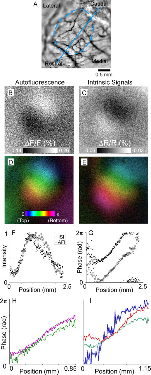
Responses in mouse primary visual cortex to a drifting horizontal bar. A, Mouse cortex imaged through the skull using green light to highlight the cortical vascular pattern. The dashed blue oval shows the approximate boundary of primary visual cortex. The blue line shows the transect along which the measurements shown in F and G were made. B, The pattern of flavoprotein autofluorescence in mouse V1 generated in response to a horizontal bar stimulus near the top of the visual field. Bright areas are active. C, The pattern of intrinsic signals in the same imaged field in response to the same bar stimulus. Dark areas are active. Images in B and C were linearly contrast stretched to fill the dynamic range. D, The retinotopic organization of mouse V1 mapped using autofluorescence imaging. The color bar shows the mapping of the stimulus monitor onto the cortical surface. E, The same retinotopic organization mapped with intrinsic signal imaging. F, Relative response strength measured along the path shown in A. Responses are normalized to the peak along the same transect. G, Phase of responses as a function of distance. The phase represents the retinotopic location that best activated a given point in the map. H, Phase of responses for three identical bar stimuli in the same mouse. I, Phase of responses for three identical bar stimuli in three other mice. The traces have been shifted in the y-axis to demonstrate slope.

We visualized the retinotopic organization of mouse V1 by color-coding each pixel according to the location in the visual field that best activated it. These retinotopic maps for mouse V1 were produced using the method of Kalatsky and Stryker (2003), in which a bar drifted across the visual field with a fixed period, and the stimulus was repeated multiple times. The visual cortex responded with the same period as the stimulus, but responses at different retinotopic locations were out of phase with each other because the stimulus passed each location at a different time. A Fourier analysis of the light signal at each point on the cortical surface provides the strength and phase of responses at the stimulus frequency. Because retinotopic location is mapped continuously onto mouse V1, a bar drifting downward through the visual field produces a wave of activity beginning in the caudal end, which spreads rostrally through visual cortex; thus, by coding locations on the stimulus screen with a spectrum of colors, a retinotopic map is represented as a rainbow from caudal to rostral corresponding to the locations on the stimulus screen from top to bottom (Fig. 1D,E).

Autofluorescence imaging consistently produced clear maps of retinotopic organization (Fig. 1D shows one example map): the progression from upper to lower visual field is mapped smoothly from the caudal to the rostral edge of V1, comparable with well established maps defined by electrophysiology and ISI (Wagor et al., 1980; Schuett et al., 2002; Kalatsky and Stryker, 2003; Tohmi et al., 2006). The spatial boundaries of V1 are shown by the dashed line in Figure 1A, and the strength of responses to the visual stimulus is plotted in Figure 1F for both AFI and ISI along a transect through the center of V1. Figure 1G shows the phase progression along the same transect (Fig. 1H shows the progression for three separate experiments in one animal; Fig. 1I shows the progression from three other mice). The similarity in the plots of relative response strength and phase between AFI and ISI maps suggests that both techniques reveal the same area boundaries and map retinotopic location similarly.

Cortical maps in cats

The primary visual cortex in higher mammals has a more complex organization than that found in mouse V1, including maps of orientation, ocular dominance, and spatial frequency preference (Hubener et al., 1997). Such maps have been confirmed repeatedly using ISI (Bonhoeffer and Grinvald, 1991, 1993a,b; Bonhoeffer et al., 1995; Hubener et al., 1997) and voltage-sensitive dyes (Shoham et al., 1999; Sharon and Grinvald, 2002; Slovin et al., 2002), and tuning properties determined from imaging have been confirmed with electrophysiology (Crair et al., 1997; Maldonado et al., 1997; Dragoi et al., 2000; Issa et al., 2000; Trachtenberg et al., 2000). To date, however, these complex parameter maps have not been obtained with autofluorescence imaging (Shibuki and Hishida, 2004). To demonstrate that AFI can indeed be used to image the cortical organization of large mammals, we mapped orientation preference in the cat.

Figure 2 shows responses in cat area 17 to drifting horizontal (Fig. 2A) and vertical (Fig. 2B) square-wave gratings. Because fluorescence increases with activity, the brightness of a pixel in Figure 2 is proportional to the underlying neural response. Consistent with previous maps of orientation selectivity using other methods, the regions activated by the orthogonal orientations are nearly complementary (Bonhoeffer and Grinvald, 1991; Nelson and Katz, 1995; Hubener et al., 1997; Shoham et al., 1999; Kenet et al., 2003). The X's in Figure 2 mark the same locations across images and show that the locations active in response to 0° are silent in response to 90° gratings. This complementary pattern is not an artifact of normalization, because the images are normalized by a “blank” image (the response to a mean luminance gray stimulus), not by other functional images (for example, responses to orthogonal orientations) that have a native structure.

Figure 2.

Single-condition responses in cat primary visual cortex imaged by flavoprotein autofluorescence. A, Fluorescence changes in response to a horizontal square-wave grating (inset). Bright areas correspond to increases in activity and therefore show 0° iso-orientation domains. B, Fluorescence changes in response to a vertical grating; bright regions show 90° iso-orientation domains. X's mark identical locations in A and B.

Color-coded orientation preference maps generated by ISI and AFI are shown in Figure 3. The AFI responses have the well described characteristics of orientation maps: orientation preference changes smoothly across the cortical surface except for small linear fractures and pinwheel-center singularities (an additional example is shown in supplemental Fig. 3, available at www.jneurosci.org as supplemental material). To confirm that the structure of the orientation map imaged by AFI is statistically similar to that measured by ISI, we calculated the difference in orientation preference measured by the two methods (Fig. 3 E,F for the two experiments shown in Fig. 3A–D). The distributions show that AFI produces an orientation map similar to that produced by ISI: >70% of pixels in the AFI map had orientation preferences within 45° of that in the ISI map.

Figure 3.

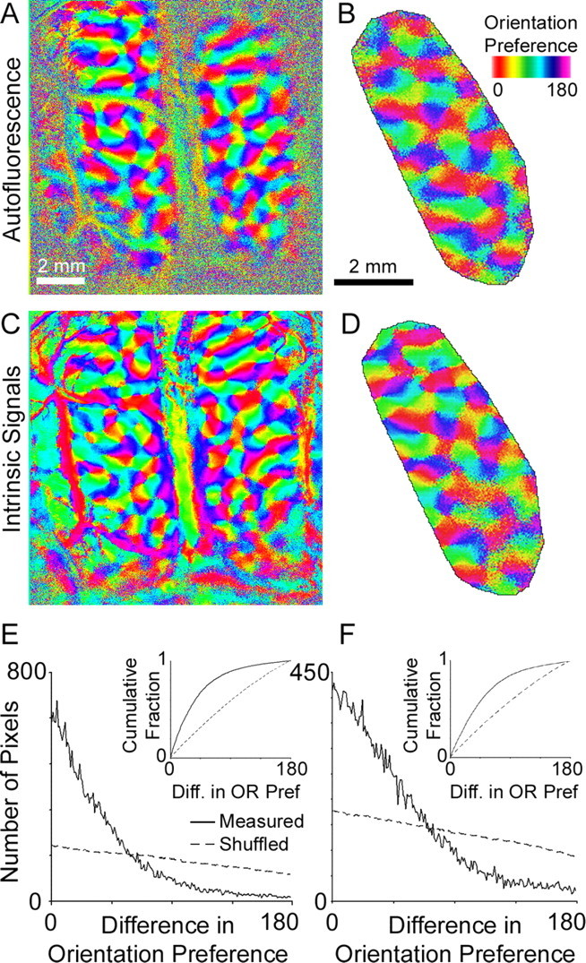
Maps of orientation preference in cat primary visual cortex generated using AFI and ISI. A, Maps of orientation preference in cat area 17 generated with AFI in the same field shown in Figure 2. B, An AFI orientation map in one hemisphere from a different animal. The imaged field has been cropped to show the region used to compare orientation preference between AFI and ISI (“templated region”). C, The same field as A mapped with ISI. D, The same field as B mapped with ISI. E, Comparison of orientation preference in the images shown in A and C. Plotted is the distribution of pixels with a given difference in orientation preference measured by AFI and by ISI (solid line). For comparison, the same distribution is plotted after shuffling the ISI map (dashed line; average distribution over 100 random shuffles). F, Comparison of orientation preference in the images shown in B and D. The insets show cumulative distribution plots for orientation difference for the measured (solid line) and shuffled (dashed line) orientation maps.

To determine whether the orientation maps are statistically similar, we calculated the difference between the measured AFI map and randomly shuffled ISI maps (the dashed lines in Fig. 3E,F plot the average difference between the AFI orientation preference map and 100 different randomized ISI orientation maps). Because randomly shuffling one of the maps preserves the distribution of orientation preference but not the structure of the orientation preference map, we can directly compare the similarity of the AFI and ISI map structure. Unlike the difference in orientation preferences measured by the two techniques, the difference between a shuffled and a measured map is nearly flat (Fig. 3E,F, dashed lines), and <35% of pixels had preferences within 45° of each other. On average, the differences between the shuffled ISI maps and the AFI maps are significantly larger than the differences between the unshuffled maps (Kolmogorov–Smirnov nonparametric test, p < 0.01; bin size = 1°, using the cumulative distributions in the inset of Fig. 3E,F). When the same distributions are plotted in polar space (supplemental Fig. 4, available at www.jneurosci.org as supplemental material), the differences between unshuffled maps are more tightly clustered around 0 than are the differences between shuffled maps, indicating that the AFI and ISI maps are very similar. Because the imaged maps are more similar to each other than expected by chance (the “shuffled” control), we conclude that AFI produces the same orientation preference map as ISI.

Spatiotemporal profile of AFI responses in cat area 17

To characterize the component of the autofluorescence signal that allows us to map cortical organization, we plotted fluorescence changes in response to visual stimuli. Figure 4A shows the increase in fluorescence in a single pixel over a horizontal-preferring orientation domain after the onset of the stimulus (the thick line shows fluorescence in response to the preferred orientation of the pixel, whereas the thin line shows fluorescence in response to the orthogonal orientation). Fluorescence in response to the preferred orientation has two components: fluorescence increases within 1 s of the onset of the preferred stimulus, and decreases below baseline within 1 s of the termination of the stimulus, but is also modulated at the frequency of respiratory ventilation. Fluorescence in response to the orthogonally oriented stimulus does not change substantially with stimulus onset, but has a large fluctuation at the frequency of artificial ventilation. For comparison, the time course of intrinsic signals is shown in Figure 4B. The intrinsic signals show the well described two-phase response consisting of increased absorption in the early phase followed by increased reflectance starting ∼6 s after stimulus onset.

Figure 4.

Visually driven response time courses in cat area 17. A, Fluorescence intensity changes during and after a 6 s visual stimulus (black bar shows the duration of the stimulus). Responses are plotted for a pixel in a horizontal-preferring orientation domain. The visual stimulus consisted of either a horizontal (thick line) or vertical (thin line) square-wave grating drifting through the visual field. The baseline intensity in the first frame of each stimulus presentation was subtracted. B, Reflectance changes at 610 nm (ISI) at a different location than the traces in A, but that had the same orientation preference. Response amplitudes have been inverted such that increases in absorbance are upward deflections. C, Plots of autofluorescence changes from the same point as in A, but after spatial high-pass filtering the images. D, Plots of reflectance changes from the same point as in B after spatial high-pass filtering the images. The traces show the mean response over 15 trials, and error bars are SEM.

The mapping signal derives from the difference between responses in the selective domains and responses in the nonselective domains. Spatial high-pass filtering accomplishes this subtraction when functional domains are small relative to the filter window (as are orientation domains). The advantages of AFI over ISI are clearest after spatial filtering, as shown in the temporal response profiles in Figure 4, C and D, and the animation of the full-imaged field in supplemental Figure 5 (available at www.jneurosci.org as supplemental material). For ISI, the mapping signal is dominated by hemodynamic factors: absorbance reaches a peak after 4 s, and then decreases (Fig. 4D) (average signal-to-noise ratio for ISI during the 6 s of stimulation is 3.0). After 6 s, reflectance increases whether the pixel is responding to its preferred orientation or the orthogonal orientation (Fig. 4D, thick and thin lines). This suggests that the late changes in absorbance are not spatially restricted, consistent with previous intrinsic signal, functional magnetic resonance imaging, and tissue oxygenation studies (Frostig et al., 1990; Malonek and Grinvald, 1996; Malonek et al., 1997; Grinvald et al., 1999; Duong et al., 2000; Shtoyerman et al., 2000; Thompson et al., 2004, 2005). In contrast, the mapping signal in AFI starts almost immediately after stimulus onset, lasts for the entire stimulus duration, and then begins to fall immediately after the stimulus ends, reaching baseline within 4 s (Fig. 4C; supplemental Fig. 5, available at www.jneurosci.org as supplemental material) (average signal-to-noise ratio for AFI during the six seconds of stimulation is 6.5). Of equal importance, fluorescence increases only in response to the preferred orientation (Fig. 4C). Therefore, unlike ISI, AFI activity is restricted to the appropriate functional domain and has a consistent spatiotemporal profile for the duration of the stimulus.

Reduced vascular artifacts

We also compared the vascular artifacts in AFI and ISI functional maps of cat visual cortex. As a measure of responsiveness to a stimulus, we used the standard deviation of intensity of a pixel in response to oriented square-wave gratings. For pixels that are strongly selective for orientation, the SD of light intensity should be high. However, if the reflectance or autofluorescence of blood vessels changes during imaging, the SD will also be high over the vasculature. The SD of light intensity is shown for one imaged field in Figure 5; the vascular pattern is shown in Figure 5A for comparison. For intrinsic signal images, the SD is highest over large blood vessels (Fig. 5C). In the same field, however, the SD of blood vessels with AFI was small compared with the responses of brain tissue (Fig. 5B). To show the full range of SDs, the images of Figure 5, B and C, were logarithmically scaled to produce Figure 5, D and E. Responses in cortex were strong in both ISI and AFI images, but vascular structures were much more prominent in the ISI image than in the AFI images. Reduced vascular artifacts make AFI functional maps, like the angle maps shown in Figure 3A and supplemental Figure 3 (available at www.jneurosci.org as supplemental material), simpler to interpret. In the AFI angle maps, coherent orientation selectivity patterns are only observed over active cortex, but in the ISI maps large, artifactual swatches of apparently coherent orientation preference appear over non-neural tissue.

Figure 5.

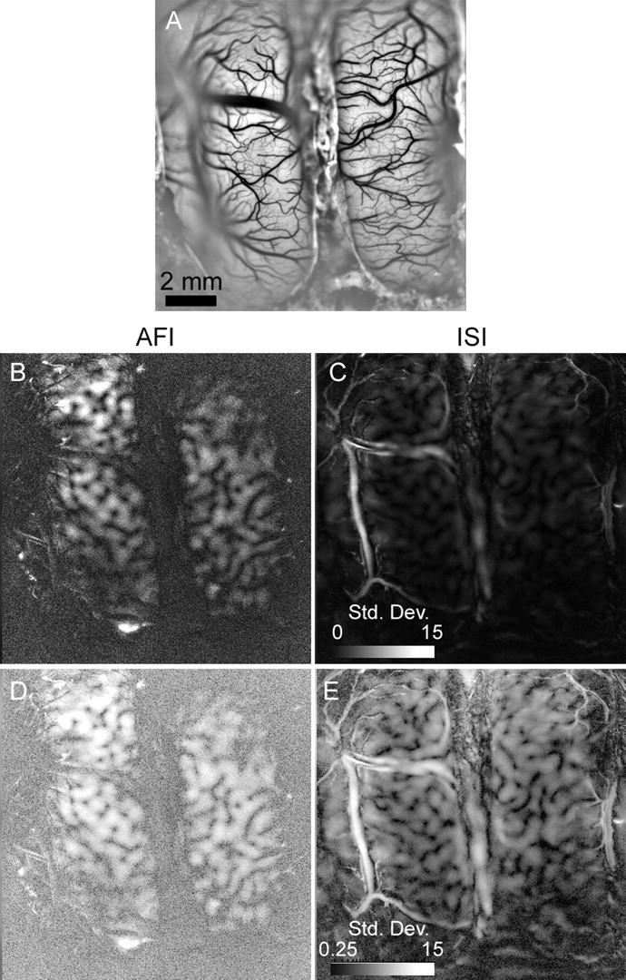
Vascular artifacts in ISI and AFI functional maps. A, The vascular pattern of the imaged field (same field as Fig. 2). The image was high-pass filtered and contrast stretched to better visualize blood vessels. B, The SD of fluorescent light intensity in AFI images generated in response to four oriented square-wave gratings. The brighter a pixel, the greater is its SD in response to the stimuli. The scale bar shows the range of SDs in blank-normalized images, multiplied by 10,000; the scale bar is applicable to B and C. C, The SD of reflected light intensity in intrinsic signal images generated in response to four oriented square-wave gratings. D, The same image as in B, but SDs have been log-scaled for better visualization. E, The same image as in C, but log-scaled. The scale bar is applicable to both D and E.

In addition, vascular outlines that run through AFI images appear qualitatively different than in ISI. In ISI images, the luminance of a vessel varies throughout its diameter, suggesting that the light absorbance of hemoglobin is changing. In AFI images, however, the variance is greatest at the vessel edges, consistent with motion artifacts. Although vasculature does contaminate AFI maps to some degree, blood vessels are not as prominent in AFI images as they are with ISI.

Improved spatial resolution

The optical point spread function, often used to determine spatial resolution, describes how an optical method induces spatial correlations in an image (the smaller spatial correlation width, the better the spatial resolution of the method). Because we cannot induce a pure point source of activity in cortex using a visual stimulus (Grinvald et al., 1994), we instead compare the spread of the optical signals when orientation domains are activated. The spatial extent of these signals was measured by calculating two-dimensional autocorrelations in images that were not spatially filtered (Fig. 6). Because the pattern of orientation domains is quasiperiodic, the autocorrelograms should show the average size and periodicity of orientation domains. As expected, the autocorrelogram generated from autofluorescence images shows a central peak with several side peaks (Fig. 6A,C). The central peak, with a full-width at half-amplitude (FWHA) of 312 μm (n = 3), is consistent with the average size of orientation domains (Rao et al., 1997). Similarly, the spacing between the central peak and side bands is ∼1 mm, the average distance between iso-orientation domains in cat area 17 (Rao et al., 1997). The autocorrelogram from intrinsic signals (Fig. 6B,D), however, shows less detail. The central peak for ISI is broader (average FWHA of 456 μm; n = 3) and lacks clear side bands, having only slight inflections at the spacing of orientation domains. This suggests that, unlike AFI images, ISI images have long-range spatial correlations that can obscure short-range modulations in intensity, even at the scale of orientation domains. Comparing the average widths of orientation domains (FWHA, 456 for ISI; 312 for AFI) suggests that AFI represents at least a 30% improvement in spatial resolution, and may be substantially better if structures smaller than an orientation domain (approaching a theoretical point source) could be measured.

Figure 6.

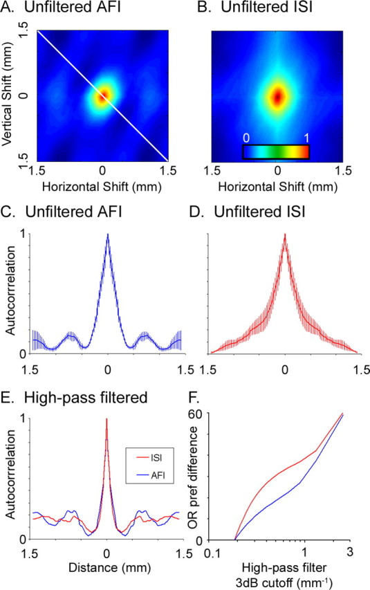
Spatial correlations in ISI and AFI orientation responses. A, B, Two-dimensional autocorrelograms averaged from three AFI (A) and three ISI (B) data sets (single-condition images were normalized but not spatially filtered). The color bar applies to A and B, and shows correlation levels from 0 (uncorrelated) to 1 (perfectly correlated). C, A plot of one transect in the spatial autocorrelogram (diagonal line in A). D, A plot of the transect through the unfiltered ISI autocorrelogram. Error bars are SEM. E, The same transects after images were high-pass filtered (AFI data in blue; ISI data in red). F, Difference in orientation preferences (in degrees) between an orientation map generated from a minimally filtered set of single-condition images (high-pass cutoff frequency, 0.185 mm⁻¹) and an orientation map generated from the same images high-pass filtered with different spatial filter cutoffs.

Single-condition images are typically high-pass filtered to produce functional maps like those of orientation preference. High-pass spatial filtering removes long-range correlations in an image (for example, it subtracts off the mean intensity of the image) accentuating high-frequency structures like orientation domains. The effect of high-pass filtering on the autocorrelograms can be seen in Figure 6E, in which the profiles for AFI and ISI are similar, and both show side peaks at the average spacing of orientation domains (images were filtered with a 70 pixel kernel, the same used to generate the orientation maps in Fig. 3). However, spatial filtering can also produce periodic modulation in an image where none exists (Rojer and Schwartz, 1990). To determine whether the structure of orientation maps produced by either AFI or ISI depends on spatial filtering, we compared orientation maps from differently filtered images. We initially used a high-pass filter with a low-frequency cutoff (in which almost all frequencies pass) to construct orientation maps, and then asked whether maps constructed using spatial filters with higher cutoffs were similar to the minimally filtered orientation map (Fig. 6F). For both intrinsic signal and autofluorescence images, the orientation preference maps were similar when the test and reference images were processed with similar filters and became progressively more different as the cutoff frequency of the filters diverged. However, orientation maps produced by autofluorescence changed less with filtering than did maps produced by intrinsic signals; the implication is that the structure of functional maps produced by autofluorescence is less dependent on postprocessing, like spatial filtering of images, than are intrinsic signal maps.

Time course of AFI responses

With any indirect measure of neural activity, one would expect a lag between activation and the peak of the measured response. The visually driven responses in cat area 17 suggest that autofluorescence changes rapidly with stimulus (Fig. 4). To better characterize the temporal response of AFI, we measured the response lag in three different ways. Initially, we estimated the delay from visual stimulus to response peak in the mouse using the “phase-reversal” method outlined by Kalatsky and Stryker (2003), in which retinotopy phase maps (like those shown in Fig. 1D,E) are generated in response to horizontal bars drifting up, and also to bars drifting down. The retinotopic maps should be the same (after correcting for opposite drift directions), except for the response lag (phase_down − phase_up = 2 × lag). This calculation gave an estimate of lag for intrinsic signal imaging of 1.0 and 0.8 s for autofluorescence.

We next measured the average onset and relaxation time of the fluorescence signal in response to a brief (200 ms) train of electrical pulses. Figure 7A shows the AFI response profile of one pixel in mouse V1 to many cycles of electrical stimulation. The autofluorescence reached a peak at 1 s, the peak was maintained for ∼0.5 s, and then decayed to baseline within 2 s followed by a transient decrease in fluorescence.

Figure 7.

AFI and absorption signal time courses in response to brief electrical stimulation in mouse. A–D, Time course of a single pixel in mouse visual cortex in response to electrical stimulation demonstrating autofluorescence signal (420–490 nm excitation filter; 520+ nm emission filter) (A), blue absorption signal (420–490 nm excitation filter, no emission filter) (B), green absorption signal (530–550 nm excitation filter; no emission filter) (C), and red absorption signal (600–620 nm excitation filter; no emission filter) (D). Each time course is from a single pixel and is the average of 22 cycles of stimulation. Error bars are SEM.

The early time course of fluorescence was similar in the cat. Fluorescence reached a peak within 1 s of the electrical stimulus and fell to near baseline within 2.5 s (Fig. 8A). In two of three experiments, however, there was a second, delayed peak of fluorescence (supplemental Fig. 7A, available at www.jneurosci.org as supplemental material). The second peak started 5–6 s after the stimulus and had an amplitude that increased as the interstimulus duration increased. At the longest interstimulus period studied (34 s), the amplitude of the second peak grew to two to three times the size of the initial peak (supplemental Fig. 7B, available at www.jneurosci.org as supplemental material). This suggests that, when present, the second peak has a very long decay phase, and that with high-frequency stimulation (>0.3 Hz) fluorescence does not return to baseline before the next cycle starts. Nonetheless, stimulation at 0.3 Hz produced a clear waveform consisting of only the first peak (data not shown).

Figure 8.

AFI and absorption signal time courses in response to brief electrical stimulation in cat. A–D, Time course of a single pixel in cat visual cortex in response to electrical stimulation demonstrating autofluorescence signal (A), blue absorption signal (B), green absorption signal (C), and red absorption signal (D). Each time course is from a single pixel and is the average of 22 cycles of stimulation. Error bars are SEM.

Finally, we measured the time course of responses in the mouse to a brief visual stimulus consisting of a full-field flash (200 ms duration). Responses to the visual stimulus were noisier than responses to the electrical stimulus, but showed a similar time to peak (Fig. 9). The fluorescence increased to a peak after 1 s, stayed elevated for 0.5–1 s, and then relaxed below baseline in another second. The results of both electrical and visual stimulation experiments are therefore consistent with the 1 s lag of AFI measured in the mouse cerebellum (Reinert et al., 2004) and previously in mouse visual cortex (Tohmi et al., 2006).

Figure 9.

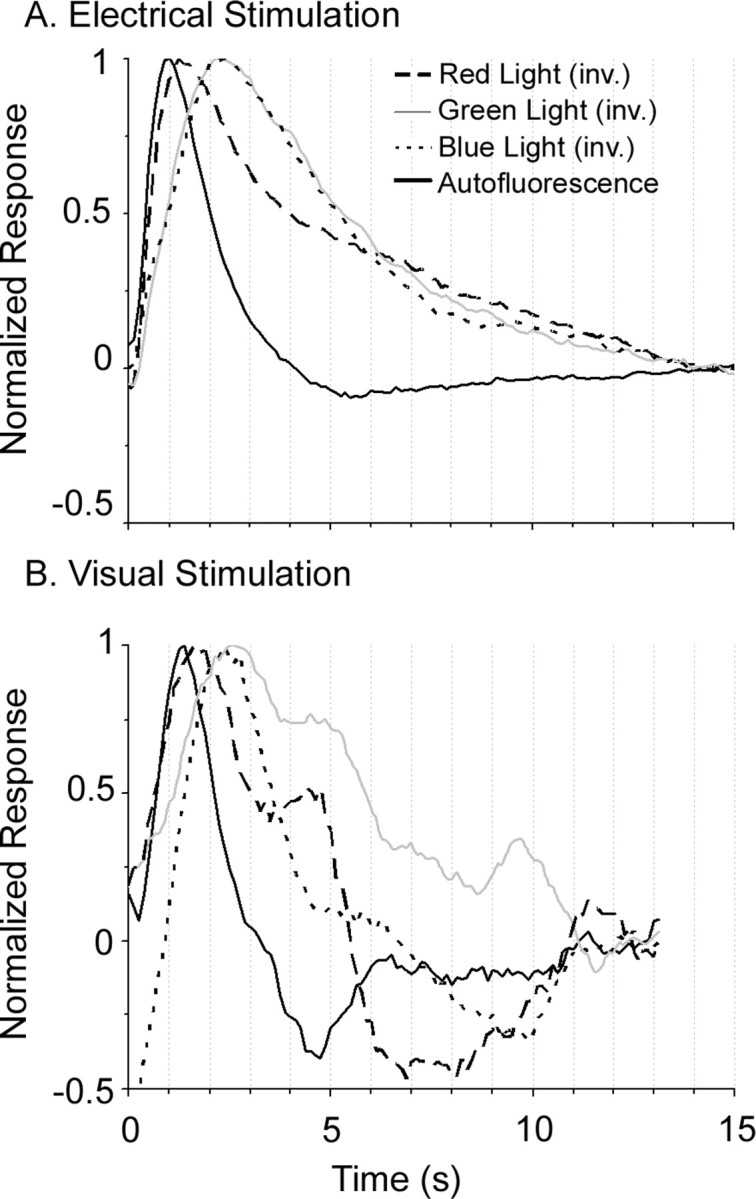
Visually and electrically driven AFI and absorption signal profiles. A, B, Time courses for the autofluorescence signal and potential intrinsic signal contaminants (all of which were inverted for direct comparison) for electrical (A) and visual (B) stimulation. Each trace is the average response over a 3 × 3 pixel region and is averaged over 22 cycles of stimulation.

Ruling out hemodynamic contamination of the fluorescence signal

Spectroscopic studies of cortical reflectance have shown that activity modulates light absorption over a wide range of wavelengths, including the excitation wavelength used to image autofluorescence (Shtoyerman et al., 2000). If the wavelength cutoffs of the excitation and emission filters are not well separated, excitation light might bleed through and contaminate the optical responses. Changes in light absorbance attributable to hemodynamics or oxy/deoxyhemoglobin absorption would therefore be confused with autofluorescence. We performed three controls to rule out this possibility.

First, we experimentally confirmed that the excitation and emissions filters are well separated: only 0.019% of the excitation light is transmitted through the emissions filter. Because this is not an epifluorescence system (that is, the excitation and emission light paths are separate), there is no chance that a poor dichroic mirror is allowing light to bleed through. The excellent separation of excitation and emission wavelengths makes bleed-through an unlikely source for the activity-dependent increases in light intensity.

Second, we imaged cortical activity using reflectance at a variety of wavelengths (and with no emission filter), including the excitation wavelengths of flavoprotein autofluorescence (420–490 nm), wavelengths near the isosbestic point of hemoglobin (530–550 nm), and the wavelengths used for ISI (600–620 nm). This is effectively the same as performing intrinsic signal imaging experiments with different illumination wavelengths. Responses to electrical stimulation in both mouse and cat cortex showed that the cortex gets darker (absorbance increases) with activity at all wavelengths tested (Figs. 7B–D, 8B–D; supplemental Fig. 7, available at www.jneurosci.org as supplemental material). This is the opposite of the fluorescence signal, in which the cortex becomes brighter with activity (Figs. 7A, 8A; supplemental Fig. 8, available at www.jneurosci.org as supplemental material). Because an increase in fluoresced light cannot be caused by bleed-through of a signal in which reflected light decreases, the opposite luminance profiles rule out the possibility that the autofluorescence signals are artifacts of blood absorbance signals.

Finally, we compared the time course of the autofluorescence response to the time course of these absorbance signals. As Figure 9 shows, the autofluorescence signal peaked earlier than absorbance signals at any of the three wavelengths tested. Although the absorbance changes are noisy after 2 s, they are clearly different from the responses of the autofluorescence signal throughout the period. The rapid increase in fluorescence is consistent with previous studies of autofluorescence (Tohmi et al., 2006), and provides additional evidence that AFI and hemodynamics are distinct signals.

Discussion

Flavoprotein autofluorescence represents an opportunity to more closely relate cellular metabolism with neural activity, with the added advantages of reduced vascular artifacts, improved spatial resolution, limited dependence on spatial filtering, a faster time course, and a spatially restricted response profile throughout the stimulus period. We showed that flavoprotein autofluorescence can be used to image the organization of cat primary visual cortex, and that the maps produced by AFI match those produced by the well established method of intrinsic signal imaging with the above improvements. Given its advantages, AFI may enable a variety of experiments related to sensory coding, cortical processing, and neurometabolic coupling in large mammals without the use of dyes.

Source of autofluorescence signal

Several studies have shown that green fluorescence in blue light is a result of the oxidation of flavoproteins (Shibuki et al., 2003; Murakami et al., 2004; Reinert et al., 2004); however, it is well known that absorption changes resulting from neural activity take place at a variety of wavelengths, including the excitation and emission frequencies of AFI (Shtoyerman et al., 2000; Jones et al., 2001; Berwick et al., 2005). Previous reports indicate that contamination from intrinsic signals is negligible in cerebellar cortex, and blocking nitric oxide synthase (which is thought to underlie the hemodynamic response) showed no significant changes in the AFI signal (Reinert et al., 2004). Likewise, several controls confirm that the autofluorescence signals we observed in primary visual cortex of mouse and cat were not artifacts of hemodynamic factors. Specifically, the hemodynamic absorption signals measured at a variety of wavelengths had the opposite sign and were slower than the autofluorescence signal. Furthermore, there are regions of the cortex in which ISI maps were strong but AFI signals were absent, suggesting that strong hemodynamic signals do not by themselves produce AFI responses. This can be seen most clearly over the blood vessels of cat cortex where hemodynamic signals (ISI) are the strongest but where there is little or no modulation in the autofluorescence signal (Fig. 5). Nevertheless, we cannot completely rule out the possibility that hemodynamic absorption signals contaminate the AFI responses, especially after the small time window during which autofluorescence increases but absorption has not changed. It may be possible using advanced temporal filtering or two-photon microscopy techniques to completely eliminate hemodynamic contributions and thus improve the temporal resolution of the AFI signal.

Moreover, it is likely that cortical flavoprotein autofluorescence measures neuronal, rather than glial, metabolism. During increased neural activity, neurons first meet energy demands by relying on their internal supply of glucose to feed the tricarboxylic acid cycle through glycolysis. Nearby astrocytes, which ensheath synaptic contacts, respond to high glutamate concentrations by producing lactate, which in turn is transported to neurons where it enters the tricarboxylic acid cycle (Magistretti and Pellerin, 1999). Because the production of lactate in astrocytes does not involve oxidation of flavoproteins, we do not expect astrocytic flavoproteins to fluoresce in response to increased neuronal activity. In neurons, however, flavoproteins are oxidized in both initial oxidative metabolism and subsequent lactate metabolism (Schurr, 2006), so the AFI signal is likely localized to active neurons. This is consistent with pharmacological experiments in mouse cerebellum in which blockade of postsynaptic glutamate receptors blocked fluorescence changes (Reinert et al., 2004), arguing for a neuronal rather than astrocytic source for flavoprotein autofluorescence.

Properties of the AFI signal: spatial resolution

Because the source of AFI is mitochondrial, we would expect AFI responses to be independent of hemodynamics. Indeed, we find that AFI maps are less contaminated by vasculature than are ISI maps (Fig. 5). A recent reanalysis of some ISI images suggested that certain cortical structures identified by ISI, like specific spatial frequency domains, tend to align with blood vessels (Sirovich and Uglesich, 2004), but because ISI relies on hemodynamic changes it is not clear whether these structures have a neural or vascular basis. Because flavoprotein autofluorescence is virtually independent of hemodynamics, AFI maps would be able to distinguish whether such correlations between functional structures and blood vessels are artifactual or genuine. Furthermore, the strength of ISI responses, as well as spatial resolution, varies across cortical areas in proportion to the density of the vascular bed in each area (Harrison et al., 2002), limiting the usefulness of ISI to areas, like primary visual cortex, with a high density of capillaries. AFI may therefore be especially useful in imaging responses in cortical areas in which ISI images are weak. Because of the reduced dependence on blood flow, and therefore reduced vascular contamination, AFI is better suited to producing accurate maps of fine cortical organization.

In addition to reduced signal directly over blood vessels, AFI also has better spatial resolution than blood-based signals, as shown by the tighter autocorrelation profile in AFI images (Fig. 6). This finding has several implications for neurovascular coupling and functional imaging. First, even the early “specific” phase of intrinsic signals is not localized to just active neural areas. Second, AFI images are less dependent on postprocessing than are ISI images. All functional maps from ISI require high-pass spatial filtering [or, alternatively, temporal filtering with a narrow bandpass in the case of phase-encoded imaging (Kalatsky and Stryker, 2003; Kalatsky et al., 2005)]. Unless the approximate spacing of functional domains is known before processing, it is unlikely that ISI images would reveal active patterns; even the well known orientation pinwheel pattern does not emerge from unfiltered intrinsic signal images. In contrast, AFI maps do not change as much with varying filter settings, and the spacing of orientation domains is evident even in unfiltered images (Fig. 6). Thus, although both methods represent cortical activity well at the spatial scale of orientation domains after filtering (Fig. 6E), AFI responses have a better spatial resolution and are less sensitive to postprocessing.

Equally important, autofluorescence imaging has a better spatial response profile than ISI because it remains restricted to active domains throughout its time course (Fig. 4). In comparison, intrinsic signals are centered on active domains only during the first few seconds of a response, after which a much larger area of the vascular bed is engaged. Together with the large-scale spatial correlations found in ISI images but not AFI images, these findings suggest that flavoprotein autofluorescence is a more faithful indicator of the spatial structure of cortical activity.

Properties of the AFI signal: time course of responses

The time course of visually driven autofluorescence is well behaved in both mouse and cat visual cortex. The rapid onset and relaxation with both visual and electrical stimulation suggest that autofluorescence imaging would provide a substantial improvement in temporal resolution over intrinsic signal imaging, especially in the cat. There are two practical benefits to the improved temporal response profile. First, because the AFI signal decays to baseline within 2 s of the end of the stimulus (Fig. 7A), the interstimulus interval can be shortened to 2 s, reducing imaging time by 40–50% over current ISI protocols. Second, and more important, the unimodal step response function of autofluorescence (Fig. 4C) means that qualitatively different imaging protocols can potentially be used. Most ISI experiments are performed with an episodic design, in which individual stimulus conditions are presented separately and with long interstimulus intervals. Such protocols are necessary for ISI because the hemodynamic response is nonlinearly coupled to neuronal activity. There are two temporal components to the hemodynamic response, each opposite in polarity, so it would be impossible to extract response profiles to rapidly changing or overlapping stimuli. However, because visually driven AFI signals have unimodal temporal responses that are restricted to active domains, it becomes feasible to image cortical activity in response to continuously changing or temporally overlapping stimuli. Protocols commonly used for electrophysiology, like reverse or spatial correlation studies, could potentially be accommodated by AFI, allowing the examination of information processing over large cortical regions.

Benefits and limitations of AFI

Although AFI can produce high-quality maps of cortical organization, it is important to note that the fluorescence signal is low amplitude and is very sensitive to illumination level, making mapping of large cortical areas somewhat challenging. In our setup, this required the use of two illumination sources and long integration times (200 ms) to capture sufficient fluorescence. Ultimately, the primary advantage of AFI is that it brings the mapping signal one step closer to neural activity, allowing the investigation of population responses over a large cortical region in visual mammals with improved spatial and temporal resolution.

References

- Berwick et al., 2005.Berwick J, Johnston D, Jones M, Martindale J, Redgrave P, McLoughlin N, Schiessl I, Mayhew JE. Neurovascular coupling investigated with two-dimensional optical imaging spectroscopy in rat whisker barrel cortex. Eur J Neurosci. 2005;22:1655–1666. doi: 10.1111/j.1460-9568.2005.04347.x. [DOI] [PubMed] [Google Scholar]
- Blasdel and Salama, 1986.Blasdel GG, Salama G. Voltage-sensitive dyes reveal a modular organization in monkey striate cortex. Nature. 1986;321:579–585. doi: 10.1038/321579a0. [DOI] [PubMed] [Google Scholar]
- Bonhoeffer and Grinvald, 1991.Bonhoeffer T, Grinvald A. Iso-orientation domains in cat visual cortex are arranged in pinwheel-like patterns. Nature. 1991;353:429–431. doi: 10.1038/353429a0. [DOI] [PubMed] [Google Scholar]
- Bonhoeffer and Grinvald, 1993a.Bonhoeffer T, Grinvald A. The layout of iso-orientation domains in area 18 of cat visual cortex: optical imaging reveals a pinwheel-like organization. J Neurosci. 1993a;13:4157–4180. doi: 10.1523/JNEUROSCI.13-10-04157.1993. [DOI] [PMC free article] [PubMed] [Google Scholar]
- Bonhoeffer and Grinvald, 1993b.Bonhoeffer T, Grinvald A. Optical imaging of the functional architecture in cat visual cortex: the layout of direction and orientation domains. Adv Exp Med Biol. 1993b;333:57–69. doi: 10.1007/978-1-4899-2468-1_7. [DOI] [PubMed] [Google Scholar]
- Bonhoeffer and Grinvald, 1996.Bonhoeffer T, Grinvald A. Optical imaging based on intrinsic signals. In: Toga AW, Mazziotta JC, editors. Brain mapping: the methods. New York: Academic; 1996. pp. 55–97. [Google Scholar]
- Bonhoeffer et al., 1995.Bonhoeffer T, Kim DS, Malonek D, Shoham D, Grinvald A. Optical imaging of the layout of functional domains in area 17 and across the area 17/18 border in cat visual cortex. Eur J Neurosci. 1995;7:1973–1988. doi: 10.1111/j.1460-9568.1995.tb00720.x. [DOI] [PubMed] [Google Scholar]
- Brainard, 1997.Brainard DH. The Psychophysics Toolbox. Spat Vis. 1997;10:433–436. [PubMed] [Google Scholar]
- Cannestra et al., 1998.Cannestra AF, Pouratian N, Shomer MH, Toga AW. Refractory periods observed by intrinsic signal and fluorescent dye imaging. J Neurophysiol. 1998;80:1522–1532. doi: 10.1152/jn.1998.80.3.1522. [DOI] [PubMed] [Google Scholar]
- Crair et al., 1997.Crair MC, Ruthazer ES, Gillespie DC, Stryker MP. Relationship between the ocular dominance and orientation maps in visual cortex of monocularly deprived cats. Neuron. 1997;19:307–318. doi: 10.1016/s0896-6273(00)80941-1. [DOI] [PubMed] [Google Scholar]
- Dragoi et al., 2000.Dragoi V, Sharma J, Sur M. Adaptation-induced plasticity of orientation tuning in adult visual cortex. Neuron. 2000;28:287–298. doi: 10.1016/s0896-6273(00)00103-3. [DOI] [PubMed] [Google Scholar]
- Duong et al., 2000.Duong TQ, Kim DS, Ugurbil K, Kim SG. Spatiotemporal dynamics of the BOLD fMRI signals: toward mapping submillimeter cortical columns using the early negative response. Magn Reson Med. 2000;44:231–242. doi: 10.1002/1522-2594(200008)44:2<231::aid-mrm10>3.0.co;2-t. [DOI] [PubMed] [Google Scholar]
- Frostig et al., 1990.Frostig RD, Lieke EE, Ts'o DY, Grinvald A. Cortical functional architecture and local coupling between neuronal activity and the microcirculation revealed by in vivo high-resolution optical imaging of intrinsic signals. Proc Natl Acad Sci USA. 1990;87:6082–6086. doi: 10.1073/pnas.87.16.6082. [DOI] [PMC free article] [PubMed] [Google Scholar]
- Grinvald et al., 1994.Grinvald A, Lieke EE, Frostig RD, Hildesheim R. Cortical point-spread function and long-range lateral interactions revealed by real-time optical imaging of macaque monkey primary visual cortex. J Neurosci. 1994;14:2545–2568. doi: 10.1523/JNEUROSCI.14-05-02545.1994. [DOI] [PMC free article] [PubMed] [Google Scholar]
- Grinvald et al., 1999.Grinvald A, Shoham D, Shmuel A, Glaser DE, Vanzetta I, Shtoyerman E, Slovin H, Arieli A. In vivo optical imaging of cortical architecture and dynamics. In: Windhorst U, Johansson H, editors. Modern techniques in neuroscience research. New York: Springer; 1999. pp. 893–969. [Google Scholar]
- Harrison et al., 2002.Harrison RV, Harel N, Panesar J, Mount RJ. Blood capillary distribution correlates with hemodynamic-based functional imaging in cerebral cortex. Cereb Cortex. 2002;12:225–233. doi: 10.1093/cercor/12.3.225. [DOI] [PubMed] [Google Scholar]
- Hubener et al., 1997.Hubener M, Shoham D, Grinvald A, Bonhoeffer T. Spatial relationships among three columnar systems in cat area 17. J Neurosci. 1997;17:9270–9284. doi: 10.1523/JNEUROSCI.17-23-09270.1997. [DOI] [PMC free article] [PubMed] [Google Scholar]
- Issa et al., 2000.Issa NP, Trepel C, Stryker MP. Spatial frequency maps in cat visual cortex. J Neurosci. 2000;20:8504–8514. doi: 10.1523/JNEUROSCI.20-22-08504.2000. [DOI] [PMC free article] [PubMed] [Google Scholar]
- Jones et al., 2001.Jones M, Berwick J, Johnston D, Mayhew J. Concurrent optical imaging spectroscopy and laser-Doppler flowmetry: the relationship between blood flow, oxygenation, and volume in rodent barrel cortex. NeuroImage. 2001;13:1002–1015. doi: 10.1006/nimg.2001.0808. [DOI] [PubMed] [Google Scholar]
- Kalatsky and Stryker, 2003.Kalatsky VA, Stryker MP. New paradigm for optical imaging: temporally encoded maps of intrinsic signal. Neuron. 2003;38:529–545. doi: 10.1016/s0896-6273(03)00286-1. [DOI] [PubMed] [Google Scholar]
- Kalatsky et al., 2005.Kalatsky VA, Polley DB, Merzenich MM, Schreiner CE, Stryker MP. Fine functional organization of auditory cortex revealed by Fourier optical imaging. Proc Natl Acad Sci USA. 2005;102:13325–13330. doi: 10.1073/pnas.0505592102. [DOI] [PMC free article] [PubMed] [Google Scholar]
- Kenet et al., 2003.Kenet T, Bibitchkov D, Tsodyks M, Grinvald A, Arieli A. Spontaneously emerging cortical representations of visual attributes. Nature. 2003;425:954–956. doi: 10.1038/nature02078. [DOI] [PubMed] [Google Scholar]
- Magistretti and Pellerin, 1999.Magistretti PJ, Pellerin L. Cellular mechanisms of brain energy metabolism and their relevance to functional brain imaging. Philos Trans R Soc Lond B Biol Sci. 1999;354:1155–1163. doi: 10.1098/rstb.1999.0471. [DOI] [PMC free article] [PubMed] [Google Scholar]
- Maldonado et al., 1997.Maldonado PE, Godecke I, Gray CM, Bonhoeffer T. Orientation selectivity in pinwheel centers in cat striate cortex. Science. 1997;276:1551–1555. doi: 10.1126/science.276.5318.1551. [DOI] [PubMed] [Google Scholar]
- Malonek and Grinvald, 1996.Malonek D, Grinvald A. Interactions between electrical activity and cortical microcirculation revealed by imaging spectroscopy: implications for functional brain mapping. Science. 1996;272:551–554. doi: 10.1126/science.272.5261.551. [DOI] [PubMed] [Google Scholar]
- Malonek et al., 1997.Malonek D, Dirnagl U, Lindauer U, Yamada K, Kanno I, Grinvald A. Vascular imprints of neuronal activity: relationships between the dynamics of cortical blood flow, oxygenation, and volume changes following sensory stimulation. Proc Natl Acad Sci USA. 1997;94:14826–14831. doi: 10.1073/pnas.94.26.14826. [DOI] [PMC free article] [PubMed] [Google Scholar]
- Murakami et al., 2004.Murakami H, Kamatani D, Hishida R, Takao T, Kudoh M, Kawaguchi T, Tanaka R, Shibuki K. Short-term plasticity visualized with flavoprotein autofluorescence in the somatosensory cortex of anaesthetized rats. Eur J Neurosci. 2004;19:1352–1360. doi: 10.1111/j.1460-9568.2004.03237.x. [DOI] [PubMed] [Google Scholar]
- Nelson and Katz, 1995.Nelson DA, Katz LC. Emergence of functional circuits in ferret visual cortex visualized by optical imaging. Neuron. 1995;15:23–34. doi: 10.1016/0896-6273(95)90061-6. [DOI] [PubMed] [Google Scholar]
- Pelli, 1997.Pelli DG. The VideoToolbox software for visual psychophysics: transforming numbers into movies. Spat Vis. 1997;10:437–442. [PubMed] [Google Scholar]
- Rao et al., 1997.Rao SC, Toth LJ, Sur M. Optically imaged maps of orientation preference in primary visual cortex of cats and ferrets. J Comp Neurol. 1997;387:358–370. doi: 10.1002/(sici)1096-9861(19971027)387:3<358::aid-cne3>3.3.co;2-v. [DOI] [PubMed] [Google Scholar]
- Reinert et al., 2004.Reinert KC, Dunbar RL, Gao W, Chen G, Ebner TJ. Flavoprotein autofluorescence imaging of neuronal activation in the cerebellar cortex in vivo. J Neurophysiol. 2004;92:199–211. doi: 10.1152/jn.01275.2003. [DOI] [PubMed] [Google Scholar]
- Rojer and Schwartz, 1990.Rojer AS, Schwartz EL. Cat and monkey cortical columnar patterns modeled by bandpass-filtered 2D white noise. Biol Cybern. 1990;62:381–391. doi: 10.1007/BF00197644. [DOI] [PubMed] [Google Scholar]
- Schuett et al., 2002.Schuett S, Bonhoeffer T, Hubener M. Mapping retinotopic structure in mouse visual cortex with optical imaging. J Neurosci. 2002;22:6549–6559. doi: 10.1523/JNEUROSCI.22-15-06549.2002. [DOI] [PMC free article] [PubMed] [Google Scholar]
- Schurr, 2006.Schurr A. Lactate: the ultimate cerebral oxidative energy substrate? J Cereb Blood Flow Metab. 2006;26:142–152. doi: 10.1038/sj.jcbfm.9600174. [DOI] [PubMed] [Google Scholar]
- Sharon and Grinvald, 2002.Sharon D, Grinvald A. Dynamics and constancy in cortical spatiotemporal patterns of orientation processing. Science. 2002;295:512–515. doi: 10.1126/science.1065916. [DOI] [PubMed] [Google Scholar]
- Shibuki and Hishida, 2004.Shibuki K, Hishida R. Physiology online, issue 54 edition. London: The Physiological Society; 2004. Flavoprotein autofluorescence. [Google Scholar]
- Shibuki et al., 2003.Shibuki K, Hishida R, Murakami H, Kudoh M, Kawaguchi T, Watanabe M, Watanabe S, Kouuchi T, Tanaka R. Dynamic imaging of somatosensory cortical activity in the rat visualized by flavoprotein autofluorescence. J Physiol (Lond) 2003;549:919–927. doi: 10.1113/jphysiol.2003.040709. [DOI] [PMC free article] [PubMed] [Google Scholar]
- Shoham et al., 1999.Shoham D, Glaser DE, Arieli A, Kenet T, Wijnbergen C, Toledo Y, Hildesheim R, Grinvald A. Imaging cortical dynamics at high spatial and temporal resolution with novel blue voltage-sensitive dyes. Neuron. 1999;24:791–802. doi: 10.1016/s0896-6273(00)81027-2. [DOI] [PubMed] [Google Scholar]
- Shtoyerman et al., 2000.Shtoyerman E, Arieli A, Slovin H, Vanzetta I, Grinvald A. Long-term optical imaging and spectroscopy reveal mechanisms underlying the intrinsic signal and stability of cortical maps in V1 of behaving monkeys. J Neurosci. 2000;20:8111–8121. doi: 10.1523/JNEUROSCI.20-21-08111.2000. [DOI] [PMC free article] [PubMed] [Google Scholar]
- Sirovich and Uglesich, 2004.Sirovich L, Uglesich R. The organization of orientation and spatial frequency in primary visual cortex. Proc Natl Acad Sci USA. 2004;101:16941–16946. doi: 10.1073/pnas.0407450101. [DOI] [PMC free article] [PubMed] [Google Scholar]
- Skoog, 1985.Skoog DA. Ed 3. Philadelphia: CBS College Publishing; 1985. Principles of instrumental analysis. [Google Scholar]
- Slovin et al., 2002.Slovin H, Arieli A, Hildesheim R, Grinvald A. Long-term voltage-sensitive dye imaging reveals cortical dynamics in behaving monkeys. J Neurophysiol. 2002;88:3421–3438. doi: 10.1152/jn.00194.2002. [DOI] [PubMed] [Google Scholar]
- Takahashi et al., 2006.Takahashi K, Hishida R, Kubota Y, Kudoh M, Takahashi S, Shibuki K. Transcranial fluorescence imaging of auditory cortical plasticity regulated by acoustic environments in mice. Eur J Neurosci. 2006;23:1365–1376. doi: 10.1111/j.1460-9568.2006.04662.x. [DOI] [PubMed] [Google Scholar]
- Thompson et al., 2004.Thompson JK, Peterson MR, Freeman RD. High-resolution neurometabolic coupling revealed by focal activation of visual neurons. Nat Neurosci. 2004;7:919–920. doi: 10.1038/nn1308. [DOI] [PubMed] [Google Scholar]
- Thompson et al., 2005.Thompson JK, Peterson MR, Freeman RD. Separate spatial scales determine neural activity-dependent changes in tissue oxygen within central visual pathways. J Neurosci. 2005;25:9046–9058. doi: 10.1523/JNEUROSCI.2127-05.2005. [DOI] [PMC free article] [PubMed] [Google Scholar]
- Tohmi et al., 2005.Tohmi M, Takahashi K, Kitaura H, Kudoh M, Shibuki K. Transcranial autofluorescence imaging of cortical plasticity induced by monocular deprivation in the mouse primary visual cortex. Soc Neurosci Abstr. 2005;31:979–978. [Google Scholar]
- Tohmi et al., 2006.Tohmi M, Kitaura H, Komagata S, Kudoh M, Shibuki K. Enduring critical period plasticity visualized by transcranial flavoprotein imaging in mouse primary visual cortex. J Neurosci. 2006;26:11775–11785. doi: 10.1523/JNEUROSCI.1643-06.2006. [DOI] [PMC free article] [PubMed] [Google Scholar]
- Trachtenberg et al., 2000.Trachtenberg JT, Trepel C, Stryker MP. Rapid extragranular plasticity in the absence of thalamocortical plasticity in the developing primary visual cortex. Science. 2000;287:2029–2032. doi: 10.1126/science.287.5460.2029. [DOI] [PMC free article] [PubMed] [Google Scholar]
- Ts'o et al., 1990.Ts'o DY, Frostig RD, Lieke EE, Grinvald A. Functional organization of primate visual cortex revealed by high resolution optical imaging. Science. 1990;249:417–420. doi: 10.1126/science.2165630. [DOI] [PubMed] [Google Scholar]
- Tusa et al., 1978.Tusa RJ, Palmer LA, Rosenquist AC. The retinotopic organization of area 17 (striate cortex) in the cat. J Comp Neurol. 1978;177:213–235. doi: 10.1002/cne.901770204. [DOI] [PubMed] [Google Scholar]
- Tusa et al., 1979.Tusa RJ, Rosenquist AC, Palmer LA. Retinotopic organization of areas 18 and 19 in the cat. J Comp Neurol. 1979;185:657–678. doi: 10.1002/cne.901850405. [DOI] [PubMed] [Google Scholar]
- Wagor et al., 1980.Wagor E, Mangini NJ, Pearlman AL. Retinotopic organization of striate and extrastriate visual cortex in the mouse. J Comp Neurol. 1980;193:187–202. doi: 10.1002/cne.901930113. [DOI] [PubMed] [Google Scholar]