Spontaneous Activity of Auditory-Nerve Fibers: Insights into Stochastic Processes at Ribbon Synapses

Abstract

In several sensory systems, the conversion of the representation of stimuli from graded membrane potentials into stochastic spike trains is performed by ribbon synapses. In the mammalian auditory system, the spiking characteristics of the vast majority of primary afferent auditory-nerve (AN) fibers are determined primarily by a single ribbon synapse in a single inner hair cell (IHC), and thus provide a unique window into the operation of the synapse. Here, we examine the distributions of interspike intervals (ISIs) of cat AN fibers under conditions when the IHC membrane potential can be considered constant and the processes generating AN fiber activity can be considered stationary, namely in the absence of auditory stimulation. Such spontaneous activity is commonly thought to result from an excitatory Poisson point process modified by the refractory properties of the fiber, but here we show that this cannot be the case. Rather, the ISI distributions are one to two orders of magnitude better and very accurately described as a result of a homogeneous stochastic process of excitation (transmitter release events) in which the distribution of interevent times is a mixture of an exponential and a gamma distribution with shape factor 2, both with the same scale parameter. Whereas the scale parameter varies across fibers, the proportions of exponentially and gamma distributed intervals in the mixture, and the refractory properties, can be considered constant. This suggests that all of the ribbon synapses operate in a similar manner, possibly just at different rates. Our findings also constitute an essential step toward a better understanding of the spike-train representation of time-varying stimuli initiated at this synapse, and thus of the fundamentals of temporal coding in the auditory pathway.

Introduction

In vertebrate auditory, visual, vestibular, and electroreceptive systems, the conversion of the representation of stimuli from graded membrane potentials to stochastic trains of action potentials is performed by ribbon or ribbon-like synapses (Zhai and Bellen, 2004; Fuchs, 2005; Prescott and Zenisek, 2005; Sterling and Matthews, 2005; Moser et al., 2006). Remarkably, in the mammalian auditory system, spiking characteristics of the vast majority of auditory-nerve (AN) fibers, the primary afferents, are primarily determined by a single ribbon synapse each, although each inner hair cell (IHC) receptor contains several ribbons (Liberman et al., 1990). This provides a unique opportunity to derive important aspects of the release statistics of this synapse in an undisturbed environment, namely from the spike trains of AN fibers, if their refractory properties are known or can be estimated. More generally, it makes the IHC-AN fiber system an ideal model for studying the operation of ribbon synapses.

The simplest case in which release statistics can be studied is in the absence of auditory stimulation, when for most practical purposes and for moderately long periods of time the receptor potential can be considered constant and the processes generating AN fiber activity stationary (Geisler, 1998). It is generally assumed that excitation of AN fibers is provided by a Poisson point process, which, in the case of spontaneous activity, is homogeneous or fractal doubly stochastic, to account for rate trends and phenomena seen over longer time scales (>100 ms to tens of seconds) (Lowen and Teich 1991, 1992; Jackson and Carney, 2005) (for review, see Delgutte, 1996; Mountain and Hubbard, 1996). Both types of process lead to identical interspike-interval (ISI) distributions (Teich et al., 1990). The observed deviations from strictly exponential ISI distributions are therefore commonly attributed to the refractoriness of AN fibers. By the same rationale, the slow recovery (over tens of milliseconds) of the discharge probability with time since the last spike (Gray, 1967; Gaumond et al., 1982, 1983; Li and Young, 1993; Johnson, 1996) has also been attributed to the refractory properties (Kiang et al., 1965; Gaumond et al., 1983; Young and Barta, 1986; Carney, 1993; Li and Young, 1993; Miller and Wang, 1993; Zhang et al., 2001). However, direct studies of the refractory properties of AN fibers by means of electrical stimulation have shown that refractory periods are very short, <1 or 2 ms (Brown, 1994; Dynes, 1996; Cartee et al., 2000; Miller et al., 2001; Shepherd et al., 2004; Morsnowski et al., 2006). These data, therefore, question the common notion that the excitation of AN fibers is provided by a Poisson process.

Here, we show that a simple and physiologically plausible modification of an excitatory Poisson process, in combination with refractoriness that is consistent with the experimental data, can fully account for the observed spontaneous ISI distributions. In addition to providing new insights into the operation of ribbon synapses, our model is likely to also promote understanding of the effects of auditory stimulation on AN fiber spike trains and of constraints on temporal coding.

Materials and Methods

Five adult cats (three females, two males; weighing 3–3.5 kg) with clean tympani were used for this study. All surgical and experimental procedures were approved by the Monash University Department of Psychology Animal Ethics Committee and were performed in an electrically shielded, sound-attenuating room.

Surgery.

Cats were anesthetized with pentobarbitone sodium (40 mg/kg, i.p.) and prepared for recordings from the left AN, as described in detail previously (Heil and Irvine, 1997; Heil and Neubauer, 2001). Anesthesia was maintained throughout the experiment by intravenous injections of pentobarbitone, mixed with physiological saline containing 5% glucose. No further medication was used. The electrocardiogram was continuously monitored, and rectal temperature was held at ∼38°C by a thermostatically controlled DC blanket. A round-window electrode, allowing the compound action potential to be monitored (Rajan et al., 1991), and a length of fine-bore polyethylene tubing, allowing static pressure equalization within the middle ear, were inserted through a small hole in the bulla on the recording side. The bulla was resealed, and the external meatus cleared of surrounding tissue and transected to leave only a short meatal stub. On the recording side, the skull was trephined caudal to the tentorium, the dura was removed, and the cerebellum over the cochlear nucleus was aspirated. The AN was exposed near its exit from the internal auditory meatus.

Recording procedures.

Single AN fibers were recorded with micropipettes or, more often, with glass-insulated tungsten microelectrodes with impedances of 4–7 MΩ at 1 kHz. Signal-to-noise ratios were approximately equivalent and generally excellent. Under visual control through an operating microscope, the electrode was advanced in a dorsoposterior-to-ventroanterior and slightly medial-to-lateral direction, similar to the approach by Liberman and Kiang (1978), to contact the nerve as near to its exit from the internal auditory meatus as possible.

Acoustic stimuli were digitally produced (Tucker Davis Technology, Gainesville, FL) and presented to the cat's left ear (i.e., ipsilateral to the AN chosen for recording) via a calibrated sealed sound delivery system consisting of a STAX SRS-MK3 transducer in a coupler [Sokolich WG (1981) U.S. Patent Application 4251686, pending]. Noise and tone bursts were used as search stimuli, because some AN fibers have very low spontaneous discharge rates (Liberman and Kiang, 1978) and might have been missed otherwise. Once a fiber was encountered and well isolated (i.e., when action potentials were of large signal-to-noise ratio and clearly from a single fiber only), we determined the characteristic frequency (CF) of the fiber (the frequency to which a fiber is most sensitive) by manually varying the stimulus frequency and amplitude. Next, and for other purposes, up to 200 repetitions of tones with a given frequency (at CF first), duration, and shape of the pressure envelope (usually 100 ms, including 4.2 ms cosine-squared rise and fall times) were presented at a fixed rate (usually 4 Hz), at sound pressure levels (SPLs) increasing from low (as low as −14 dB SPL) to high values (generally 80–90 dB SPL, never exceeding 100 dB SPL) in small steps (most often 4 dB). This protocol was followed, within ∼2 s (the time required for storing the previous data on disc), by recording the spontaneous activity of the fiber over a period equal to the product of the number of repetitions and the repetition period used for the tone stimulation. Thus, with 200 repetitions presented at 4 Hz, spontaneous activity was sampled over a period of 50 s. If the recording conditions were still stable, another tone stimulus, differing from the previous one in frequency or temporal envelope, was selected and the protocol repeated. In this way, several long samples of spontaneous activity were recorded from most fibers, separated by periods during which responses to tones were recorded. In this paper, only data on spontaneous activity are presented.

The electrode signal was amplified, filtered, and passed through a Schmitt trigger. Spike times were taken as the instances at which the amplified and filtered electrode signal crossed the Schmitt trigger level and were stored on disc with 1 μs resolution for off-line analysis.

Data analysis.

For off-line analysis, spike times were imported into Excel 2000 (Microsoft, Redmond, CA) spreadsheets. Visual Basic for Applications routines were developed to compute the more complex measures and to simulate data, as explained below and in the Results. The Solver of Excel was used to fit the models to the data using the Newton procedure.

Selection of the periods of stable spontaneous rate within the samples.

The analyses presented here are restricted to periods of sufficiently stable spontaneous activity. To identify such periods, we proceeded as follows. We first plotted for each sample of spontaneous activity the cumulative sum of the ISIs as a function of ISI number in the sequence in which they were recorded. For a perfectly regular spike train of constant ISI, such a plot would result in a straight line through the origin with a slope equal to that ISI. Spike trains with random ISIs but of constant longer-term rate resulted in random fluctuations of the data points around a straight line with a slope approximately equal to the mean ISI and with an offset near zero. Longer-term fluctuations in spike rate become obvious in such plots as smooth changes in the slope of the function, and the offsets of straight line fits can deviate substantially from zero. We next performed straight-line fits to such functions for each sample and computed the RMS of the residuals for each such fit. We also separated each sample of spontaneous activity into two subsamples, one covering the first and the other the second half of the ISIs of the complete sample, and computed the mean ISI and the associated SD for each subsample. A sample of spontaneous activity had to fulfill two criteria to be considered stable. First, the difference between the means of the ISIs during the first half and the second half of the sample had to be smaller than twice their probable difference, D, given by D = (SD₁ ²/n ₁ + SD₂ ²/n ₂)^0.5, where SD₁ and SD₂ are the SDs from the first and second halves of the sample, respectively, and n ₁ and n ₂ are the corresponding numbers of ISIs. If the total number of ISIs in the sample was odd, the difference between n ₁ and n ₂ was 1; otherwise, the difference was zero. For n ₁ and n ₂ greater than ∼30, the means can be expected to be normally distributed, so this criterion has an error probability of ∼5%. In other words, ∼5% of random spike trains with stable longer-term rate can be expected to not meet this criterion. Second, the offset of the straight-line fit to the function relating the cumulative ISI to ISI number had to be smaller than 30 times the RMS value computed from the fit to all ISIs. If one or both of the two criteria were not fulfilled by a given sample, the sample was pruned until the remaining period fulfilled both criteria. If no such period existed, the entire sample was discarded. Pruning started by discarding the ISIs from the first to that at which the cumulative function first intersected the straight-line fit. If necessary, this procedure was repeated iteratively, until the remaining period fulfilled both criteria. This pruning procedure is particularly effective in removing possible rate instabilities at the beginning of the sample. All data reported here are from samples or periods of samples that passed both criteria. Of the 186 samples included in this study (see Results), 78 (42%) were pruned in this way. On average, 10.5% of the ISIs were removed by the pruning. It is worth emphasizing that we arrived at our model and our conclusions (to be described below) based on analyses of complete (unpruned) samples. The major effects of the pruning of periods of unstable rate are a reduction in the scatter of data points around model functions, such as that relating SD to mean ISI (compare Fig. 10), and a reduction in the widths of the distributions of estimated parameters.

Figure 10.

Constant values of t _D, 1/λ_R, and b can explain the tight relationship between SD and mean ISI across fibers. a, Scatterplot of the SD versus the mean ISI for 186 samples of spontaneous (spont) activity with >400 ISIs. b, Same as a, but with linear axes and restricted to values of SD and mean <45 ms for higher resolution. c, Plot of CV against mean ISI. In all three panels, the red and blue lines show the relationships expected with models II and Ia, respectively, if t _D, 1/λ_R, and b were constant across AN fibers and were as identified in a. The two yellow data points are from the study of cat AN fibers by Li and Young (1993) and represent the fibers with the highest driven rates to CTs or STBs, respectively. Note that model II, but not model Ia, predicts these points correctly and fits the data from the present study very well. Four data points from a single, extraordinary AN fiber with relatively long minimum ISI (open circles) deviate conspicuously from the tight relationship between SD and mean ISI formed by the others (black circles). See Results for details.

Model fitting to cumulative distribution functions.

For the analyses of ISI distributions, all ISIs from a given sample, or from the period of a sample that had passed the rate stability criteria, were sorted by their magnitudes and plotted as a cumulative distribution function (CDF). For convenience, these functions will be referred to as sample CDFs. To prevent the sample CDF from reaching 1 and to enable fair comparisons between sample and theoretical CDFs, a margin correction was used in the calculation of the sample CDF. To calculate the cumulative probability, P _i, of a given ISI, we used the formula P _i = i/(n + 1), where i is the rank of the ith ISI after sorting them by magnitude, and n is the total number of ISIs in the sample (Sachs, 2002).

We fitted our models directly to the sample CDFs of the ISIs, rather than to their probability density functions (PDFs) or even hazard functions (HFs). Our approach has at least two major advantages over approaches that attempt to fit the latter functions. One is accuracy, because the computation of a sample CDF does not require binning of data. In this way, no information is lost and quantization errors are kept to the unavoidable minimum resulting from the sampling rate with which the spike times were stored. The other advantage is that even with moderate numbers of ISIs in a sample, say a few hundred, CDFs are very smooth. Such sample CDFs, therefore, allow small systematic deviations of the data from a model to be readily seen. The corresponding PDFs and HFs, in contrast, are inherently much noisier, because the PDF is the derivative of the CDF, and the HF the ratio of the PDF and the survival function (i.e., 1-CDF). To reduce fluctuations in PDFs and HFs requires additional binning or smoothing operations, which both result in substantial loss of information. Even after such operations, PDFs and HFs appear much noisier than the CDFs (compare, for example, the appearances of CDFs with PDFs and HFs in Figs. 2 and 3). We therefore computed the latter functions for illustrative purposes only. It is clear, but worth emphasizing, that a model that fits a sample CDF must also fit the corresponding PDF and HF, and that a model that does not fit a sample CDF also does not fit the corresponding PDF or HF, although the mismatch may be difficult to see with the latter two functions.

Figure 2.

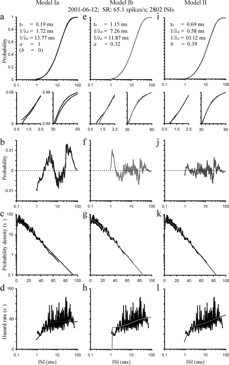
a–l, Fit of models Ia (a–d; left column), Ib (e–h; center column), and II (i–l; right column) to the sample CDF (a, e, i; top rows), the PDF (c, g, k), and the HF (d, h, l; bottom row). The subset panels in a, e, and i show blow-ups of the main panels, with the left subset from the bottom left and the right subset from the top right portion of sample and model CDFs. The best-fitting model functions are shown in gray (smooth curves) and data in black. The parameters of these functions are identified in the top panels. Sample PDFs and HFs were computed using a running average over 30 ISIs; thus, bin width varies with ISI. The center row (b, f, j) shows the residual probabilities between sample and model CDF (data minus fit). Data are for AN fiber 2001–06-12 with an SR of 65.1 spikes/s and are based on 2802 ISIs, as identified at the top of the figure. See Results for additional explanations.

Figure 3.

a–l, Same as in Figure 2, but for a different AN fiber (2001–07-08) from a different cat. Note that for the best fit of model Ib, returned identical values of 1/λ_R and 1/λ_E (within the constraints set) are shown.

To fit a given model to a sample CDF, we minimized a cost function by means of the adaptive Newton's method. For each data point, we calculated the vertical difference (in units of probability) as well as the horizontal difference (in units of time) between the sample CDF and the model CDF. The cost function was the sum of the products of the squared vertical differences and the squared horizontal differences, the latter being weighted with the survival function. The weights were introduced to prevent an undue bias by the ISIs at the upper end of the distributions in a sample, because they display the largest scatter along the horizontal axis.

The estimation of model parameters can be problematic when more than one parameter needs to be estimated simultaneously, as is the case here: the models to be tested had three or four free parameters, with two of those characterizing the refractoriness of a fiber and the other(s) the process providing the excitation to the fiber (see Results). There may be multiple solutions with similar costs, because parameters might compensate each other. Furthermore, given a particular cost function, the solution obtained may depend on the starting values to which the model parameters are set. Therefore, we developed a three-stage procedure specifically designed to guide the fitting routine in its convergence on the absolute minimum of the cost function with a reasonable combination of parameter estimates. From the first to the third stage, one, two (or three for the four-parameter models), and finally all three (or four) free parameters were optimized. The free parameter at the first stage was the time constant of the relative refractory period (RRP) (see Results for details). One (or two) of the other parameters was held constant, whereas the value of the last parameter, a scale parameter, was estimated from the mean ISI by the method-of-moments (Ayyub, 1997). The estimate was updated with every iterative step of the adaptive Newton procedure using this method. At the second stage, the time constant of the RRP and the duration of the absolute refractory period (ARP) (and a third parameter, depending on the model) were free parameters, whereas the scale parameter was again estimated, and continuously updated, from the mean ISI by the method-of-moments.

The starting values of the parameters characterizing the refractory function were selected based on existing knowledge. In a first round of fits, the starting value for the time constant of the RRP was set to 1 ms, a plausible figure according to the experimental findings described in the Introduction, and the starting value of the ARP to 90% of the shortest ISI in the sample. This choice also seemed reasonable given that the ARP, by its definition, can be expected to be shorter than the shortest ISI in the sample. The starting value for the scale parameter was calculated by the methods-of-moments from these values and from the mean ISI of the sample (see Eqs. 6, 13, and 16). For the four-parameter models, the starting value of the fourth parameter, which captures the relative proportions of different components in presumed mixtures of distributions, was set such that the starting conditions were identical to those for the three-parameter model [i.e., the starting values were a = 1 and b = 0 (for models Ib and II, respectively; see Results)]. For each model, we also performed a second round of fits in which we used as the starting value for one parameter the median across all fitted samples obtained from the initial round. For the three-parameter model, this was the time constant of the RRP, and for the four-parameter models, the parameter specifying the proportions in the mixture (i.e., a or b). Both rounds produced identical results for all, or nearly all, samples, emphasizing the reliability of the fitting procedure. These observations render it unlikely that even better solutions might have been obtained for some samples with other starting conditions, although we cannot exclude this possibility for all samples.

Evaluations of the goodness-of-fit of the different models were based on the vertical differences between the sample CDF and the model CDF (the presumed population CDF). We used the sum of the squared vertical differences as well as the maximum absolute vertical difference between sample and model CDF as key measures, because they are the basis of quadratic class statistics, such as those of the Cramér-von Mises family and of supremum class statistics, respectively (Stephens, 1986). The goodness-of-fit of a given model was further quantified by the vertical differences between sample and model CDFs to the cumulative probability averaged across all samples. The randomness-of-fit was assessed based on the shape and amplitude of this function. To allow for averaging, the vertical differences between sample and model CDF were calculated for 10,000 probability values equally spaced between 0 and 1 by linear interpolation between the observed differences as a function of the empirical cumulative probability for each sample. In this way, the differences are obtained at equal probabilities in different samples of spontaneous activity. Each difference was weighted by the square root of the number of ISIs in the sample to normalize for the fact that the magnitude of the maximum difference between a sample and a model CDF is nearly proportional to the inverse of the square root of that number (Sachs, 2002). These differences were then averaged across samples at identical probability values and divided by the mean of the square roots of the number of ISIs in the sample. These mean residuals and their associated SEs (SEM) were plotted as functions of the empirical cumulative probability for each of the models.

The meaningfulness and the reliability of the parameter estimates obtained with this fitting procedure were controlled using extensive simulations for one of the models, as explained in the Results. The fits of these sets of simulated random data (∼30,000 samples in total, with numbers of ISIs between 401 and 3411 to mimic the real data) returned parameter estimates close to the parameter values used to generate the data. The medians of the returned estimates differed from these values by 2.4% (±0.3) for the ARP, −7.2% (±0.7) for the time constant of the RRP, and −5.7% (±0.3) for the parameter specifying proportions. The evaluation of the estimates was complemented by direct comparisons of empirical values of mean ISI, SD, and coefficient of variation (CV) with those calculated from the parameter estimates returned by the fits (see Fig. 7). The parameter estimates were further controlled by applying the fitting procedure to theoretical CDFs. Theoretical CDFs were not generated as random samples but were computed from the inverse model CDF for equally spaced probabilities. These fits showed that our procedure was capable of precisely retrieving the model parameters in this condition. The medians of the parameter estimates obtained from the fits to 186 theoretical CDFs, computed with various numbers of points to mimic the real data, differed from the parameters used to generate the CDFs by <0.03%.

Figure 7.

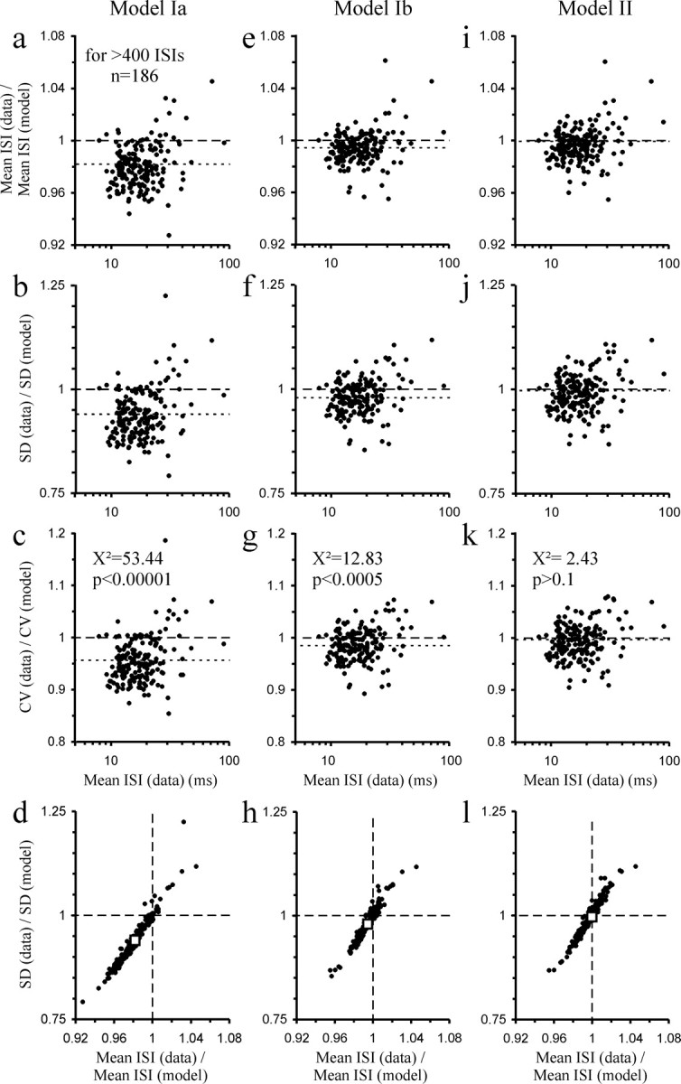
Comparison of the mean ISI, SD, and CV of the 186 samples of spontaneous activity with those predicted by the best fit of the different models. a–l, The left (a–d), center (e–h), and right columns (i–l) show the comparisons for models Ia, Ib, and II, respectively. The top row plots the ratio of the mean ISI in the data to that predicted by each model as a function of ISI; the second and third rows are the corresponding plots for SD and CV. The bottom row plots the ratio of the SDs against that of the means to illustrate their close correlations with slopes >1. The dashed lines mark ratios of 1 (i.e., data and predictions are identical). The dotted lines in the top three rows and the open squares in the bottom row represent the medians obtained from the top 19 of the 186 samples when ranked according to number of ISIs. Note that models Ia and Ib systematically overestimate mean ISI, SD, and CV, whereas model II does not. The results of χ² tests for CV are listed in the third row.

Results

Database

Spontaneous activity was recorded from 171 AN fibers from five cats. From each fiber, we obtained between 1 and 18 samples of spontaneous activity, yielding a total of 461 samples, each lasting between 12.5 and 135 s. The mean spontaneous discharge rates (mean SR) of the fibers (averaged across all unpruned samples from a given fiber) ranged from <0.1 to ∼100 Hz, covering the wide range of spontaneous rates reported in the cat and other species (Kiang et al., 1965; Walsh et al., 1972; Liberman and Kiang, 1978; Müller and Robertson, 1991; Relkin and Doucet, 1991; Yates, 1991; Gleich and Wilson, 1993; Richter et al., 1995; Köppl and Yates, 1999; Yates et al., 2000; Taberner and Liberman, 2005). The distribution of SRs was bimodal, with one maximum at ∼1 Hz (low-SR fibers) and the other at ∼40–80 Hz (high-SR fibers), in agreement with previous reports for the cat (Kiang et al., 1965; Liberman, 1978; Joris and Yin, 1992). The distribution of SRs was independent of CF, except that our sample was devoid of low-SR fibers with CFs below ∼1 kHz. The CFs of the fibers in our sample ranged from ∼0.3–40 kHz. The progressions of CF with depth of the electrode tip from the surface of the nerve were similar to those observed previously [Liberman and Kiang (1978), their Fig. 4A–E]. Together, these observations indicate that we sampled fibers from most areas of the auditory nerve (although not necessarily in each cat).

Figure 4.

Plot of the estimates of 1/λ_R against 1/λ_E obtained from the fits of model Ib. Note that in a large fraction of cases (83 of 186; 45%), the two estimates are essentially identical (symbols on or very close to the dashed line, which represents that condition).

General framework of the models and nomenclature

The goal of the present study is to provide a physiological, yet simple, model that accurately describes the distributions of ISIs derived from the spontaneous activity of AN fibers. Therefore, we take the most common existing model as a starting point. We first show its inadequacy and then develop, via a variant of this model, another model that describes the observed ISI distributions very well and with physiologically plausible values of a minimum number of parameters (four). Hence, the basic constituents of the models that are examined here are essentially the same as those used in nearly all previous accounts of AN fiber spontaneous (and driven) activity. The models assume that excitation to a fiber is provided by a stochastic point process so that excitatory events occur at random times. An excitatory event can be thought of as the release of a package of neurotransmitter from the ribbon synapse in the IHC. Each excitatory event results in a spike unless that fiber is in a refractory state. The refractory state is characterized by an ARP, during which the probability of a spike resulting from an excitatory event is zero, followed by a RRP, during which the probability of a spike resulting from an excitatory event increases monotonically toward 1. The fiber enters a refractory state after each spike, and the refractory memory extends back in time only to the last spike. Furthermore, excitatory events and refractoriness are independent. In other words, the refractory state of the fiber has no influence on release from the IHC. Although these are characteristic features of a renewal process, the analysis of ISI distributions is also meaningful if the processes were nonrenewal. For example, Teich et al. (1990) modeled longer-term rate fluctuations in long records of spontaneous activity as resulting from a fractal doubly stochastic Poisson point process. Such a process is not a renewal process, because the interevent intervals are no longer statistically independent. But the model produces the same distribution of interspike intervals as a dead-time modified homogeneous Poisson point process (Teich et al., 1990). In the following, the interval between two consecutive excitatory events will be referred to as an interevent interval (IEI). This is to be distinguished from the (observed) interval between two consecutive spikes, the ISI. The three specific variants of this general framework, to be described in more detail below, are schematically illustrated in Figure 1.

Figure 1.

Some characteristic features of the models for the distribution of ISIs examined here. Models Ia and Ib assume that the distribution of the IEIs is exponential; model II assumes that it is a mixture of an exponential and a gamma distribution. The scaling factor, λ_E, the shape factor (β), the PDF, the HF, and the mean IEI for each model are shown in the top block (excitation). Note that the PDF, with probability density plotted along a logarithmic axis, is curved, and the HF is monotonically rising when the distribution of IEIs is gamma (β = 2) or when it is a mixture of an exponential (β = 1) and a gamma distribution (center line in the two panels at right), whereas the PDF forms a straight line and the HF is constant when the distribution is exponential (β = 1). Each excitatory event is thought to result in a spike of the afferent fiber unless the fiber is refractory. The refractory functions of the three models are shown in the center block (refractoriness). The bottom row identifies the mean ISI of each model (output). See Results for additional explanations.

We will first introduce the specifics of the models and describe the results obtained with them qualitatively. The models will then be compared quantitatively, and the parameters extracted from the ultimate model will finally be examined in detail.

Model I: the IEIs are distributed exponentially

Model I makes the assumption that the excitatory events are generated by a homogeneous Poisson process. This means that the probability of an event occurring at time t (t > 0), given that the last event occurred at t = 0, is constant and thus independent of the time elapsed since the last release event. This assumption is in accord with a large number of previous studies of AN fiber activity (Kiang et al., 1965; Molnar and Pfeiffer, 1968; Schroeder and Hall, 1974; Manley and Robertson, 1976; Lütkenhöner et al., 1980; Geisler, 1981, 1998; Geisler et al., 1985; Javel, 1986; Young and Barta, 1986; Bi, 1989; Carney, 1993; Li and Young, 1993; Miller and Wang, 1993; Schmich and Miller, 1997; Zhang et al., 2001; Krishna, 2002; Kuhlmann et al., 2002) (for review, see Delgutte, 1996; Mountain and Hubbard, 1996). The CDF of the IEIs is then given by the exponential distribution as follows:

where t (in seconds) denotes the duration of the IEIs and λ_E (in s⁻¹) is the scaling factor. The PDF and the HF, in this case the constant rate λ_E, of the IEIs are shown in Figure 1. The mean IEI, 1/λ_E, is also specified there.

Variant a

In a first variant of this model (model Ia), we assume that the refractory state is composed of an ARP of duration t _D, followed by an RRP, during which the probability r(t) of a spike occurring given an excitatory event increases exponentially from 0 to 1 with time since the previous spike, with a time constant 1/λ_R, so that:

where t is the time since the previous spike. Hence, the refractory period has a random, exponential distribution with a mean duration of (t _D + 1/λ_R). This refractory function has been implemented in many previous modeling studies (Schroeder and Hall, 1974; Lütkenhöner et al., 1980; Young and Barta, 1986; Li and Young, 1993; Prijs et al., 1993; Schoonhoven et al., 1997; Meddis and O'Mard, 2005; Meddis, 2006), and its shape is in excellent agreement with recent physiological data (Brown, 1994; Miller et al., 2001; -Morsnowski et al., 2006); it is also illustrated in Figure 1.

In this scenario, the ISIs should be distributed according to a general-gamma distribution (Young and Barta, 1986; Li and Young, 1993; Lehmann, 2002), the CDF of which is given by the following:

The PDF of this general-gamma distribution is given by the following:

Generally, the HF (Gray, 1967) is the ratio of the PDF and the survival function (1−CDF), so that:

Thus, the HF for this model is easily computed with Equation 5, with F _ISI(t) and f _ISI(t) given by Equations 3 and 4, respectively. The HF describes the tendency for some event to occur at time t (t > 0, given that the last event occurred at t = 0) and is the probability density at time t renormalized by the probability that the event failed to occur before t.

According to this model, the mean ISI is the sum of three components, the ARP, the mean duration or time constant of the RRP, and the mean IEI or time constant of the presumed Poisson process generating the excitation (Fig. 1), so that:

Generally, the variance of the ISI distribution is given by the following:

For model Ia, f _ISI(t) is given by Equation 4 and μ_ISI by Equation 6, so that the SD of the ISIs takes on the simple form:

(Young and Barta, 1986) or, when expressed as a function of the mean (Li and Young, 1993):

Note that if t _D and λ_R are constant, μ_ISI approaches (t _D + 1/λ_R) and σ_ISI approaches 1/λ_R, as λ_E approaches infinity. Thus, σ_ISI decreases monotonically with decreasing μ_ISI. An increase in σ_ISI with decreasing μ_ISI below (t _D + 1/λ_R) [Li and Young (1993), their Fig. 3a] cannot occur in reality, because μ_ISI cannot be shorter than (t _D + 1/λ_R), because λ_E cannot be negative.

Probing model Ia

We evaluated whether and how well this model can account for the ISI distributions of AN fibers by fitting Equation 3 to the sample CDFs, as described in Materials and Methods, and then examining the quality of the fits. Because the difference between a sample CDF and the population CDF decreases to zero with probability 1 as n increases (the Glivenko–Cantelli theorem of probability theory), we restricted the fits to samples of stable spontaneous activity containing at least 400 spikes (n = 186). When λ_R = λ_E, the denominator in Equation 3 is zero, so that the ratio is undefined. Although this was unlikely to happen, λ_R was constrained to ≤0.99 λ_E to ensure a stable fitting procedure. In addition, λ_R and λ_E were constrained to values >0, whereas parameter t _D was unconstrained.

Figures 2 and 3 (left column) show the results of this fit of model Ia for two representative high-SR fibers (AN2001–6-12–02 and AN2001–7-08–01). At first sight and from an overview perspective (Figs. 2 a, 3 a), the model appears to provide a reasonably good description of the data; sample and model CDFs appear to correspond closely over most of the ISI ranges, because the vertical residuals (data minus fit) are all <0.02 (Figs. 2 b, 3 b). A closer look, however, reveals systematic mismatches. The residuals show an M-shape pattern as a function of ISI. Consequently, the model overestimates the proportion of short ISIs, below ∼2 ms in these and many other examples (Figs. 2 a, 3 a, left subsets), whereas it underestimates the proportion of relatively long ISIs (Figs. 2 a, 3 a, right subsets). This mismatch is a clear indication that the model does not correctly describe the distribution of spontaneous ISIs of AN fibers.

The mismatch is, of course, also seen in the PDFs and HFs. When the probability density is plotted on a logarithmic axis, the PDFs resulting from the fits fall off linearly with increasing ISI above ISIs of a few milliseconds. Scrutiny of the sample PDFs, however, reveals that the fall-offs are supralinear (Figs. 2 c, 3 c), a phenomenon also clearly observable in previously published data sets and out to the longest ISIs shown [Kiang et al. (1965), their Fig. 8.6; Molnar and Pfeiffer (1968), their Fig. 2; Manley and Robertson (1976), their Figs. 2A, 5A, 6A; Lowen and Teich (1992), their Fig. 1; Li and Young (1993), their Fig. 4h]. Similarly, the HFs of this model level off after a few milliseconds, whereas the sample HFs continue to increase out to tens of milliseconds and possibly beyond (Figs. 2 d, 3 d). The latter phenomenon has been reported widely in the literature (Gray, 1967; Gaumond et al., 1982, 1983; Young and Barta, 1986; Li and Young, 1993; Prijs et al., 1993; Johnson, 1996), and the failure of the model to capture this phenomenon has already been pointed out by Young and Barta (1986) and Li and Young (1993).

Figure 5.

Quantitative comparisons of the models. a–c, Histograms showing various measures of goodness-of-fit of the three different models as indicated below each column. The right column shows the measures for a simplified version of model II, which has only three parameters. a, The measure of goodness-of-fit is the sum of the squared vertical differences between a given sample CDF and the model CDF; in b, it is the maximum vertical difference; and in c, it is the cost function that was minimized during the fitting procedure. For each sample, the measures for models Ib and II have been normalized with respect to those for model Ia. The vertical bars represent the median and the vertical lines represent the interquartile range; the thick horizontal bars represent the medians of the measures obtained from the top 19 of the 186 samples when ranked according to number of ISIs. d, Plot of the costs of model Ib normalized to those of model Ia and plotted against the ratio of the estimates of λ_E and λ_R. The two larger symbols represent the medians, and the horizontal and vertical bars represent the interquartile ranges of the two subgroups of samples for which the estimates of λ_E and λ_R are nearly identical (triangle) or for which they differ substantially (square). e, Plot, along the abscissa, of the ratio of the costs of a simplified three-parameter version of model II to the costs of model Ia against, along the ordinate, the ratio of the costs of the full four-parameter version of model II to the costs of model Ia. The ratio between the three-parameter models is smaller than 1, indicating a better fit of the simplified model II, in 137 of 186 samples (data points left of vertical dashed line), a highly significant proportion (χ² = 21.99; p < 0.0001). The addition of the fourth parameter to obtain the full version of model II brings about further, although relatively small, improvements (distance of data points from diagonal). See Results for additional explanations.

Figure 6.

Assessments of the goodness- and randomness-of-fit. a–c, Mean and confidence intervals (±2 SEM) of the vertical differences (residual probability) between the observed probability and that predicted by the best fits of models Ia (a), Ib (b), and II (c) plotted as a function of the observed probability. Observed probabilities were obtained at 10,000 points, equally spaced along the abscissa, by linear interpolation, and mean residuals at these points were obtained by averaging the residuals across the 186 samples of stable spontaneous activity. In this way, unsystematic residuals primarily average out, whereas systematic differences remain. Note the large systematic residuals of model Ia and the much smaller residuals of model II. The goodness-of-fit, as assessed by the sum of the squared vertical (sqd. vert.) differences, is ∼30 times better for model II than for Ia, and 2.5 times better than for Ib. Arrowheads point to conspicuous features of the mean function or of the confidence limits, as explained in the Results. d–f, Analogous plots obtained from fits of models Ia (d), Ib (e), and II (f) to 186 simulated data samples generated according to model II and with fixed values of t _D, 1/λ_R, and b, t _D = 0.59 ms, 1/λ_R = 0.65 ms, and b = 0.43 and with numbers of ISIs as in the real data. Note the striking similarities with the estimates obtained from the real data. The light gray smooth M-shaped function in f represents the mean residuals obtained from fits to 162 such simulated sets of 186 samples each. It likely reflects the residuals inherent in the fitting procedure when confronted with random data. g–i, Differences between the mean vertical differences in the real data (a–c, black lines) and the procedure-inherent residuals (light gray function in f) and associated confidence interval. For model II (i), these corrected residuals are very small and confined within the 95% confidence interval, except at very low probabilities (inset). See Results for details.

Additional indications that the model may not be correct are provided by the estimates of ARP and the RRP returned by the fits. The estimates of the ARP appeared too short, and in most cases were even negative (mean t _D across the 186 estimates, −0.041 ms; median, −0.001 ms). The estimates of the RRP (mean 1/λ_R, 2.77 ms; median, 2.45 ms), in contrast, appeared too long in light of the results of direct measurements after electrical stimulation of the AN, which indicate values in the range of 0.2–1.5 ms (Parkins, 1989; Brown, 1994; Dynes, 1996; Cartee et al., 2000; Miller et al., 2001; Shepherd et al., 2004; Morsnowski et al., 2006). Such long estimates of the RRP are also incompatible with the ability of AN fibers to follow high rates of electrical stimulation with 1 spike per pulse, up to at least 800/s (Javel and Shepherd, 2000), which requires the mean refractory period to be ≤1.25 ms. Thus, in summary, based on the qualitative observations described above, it appears that model Ia does not accurately describe the distributions of ISIs from the spontaneous activity of AN fibers. Quantitative analyses supporting this conclusion are provided below.

Variant b

A conspicuous feature that indicated the inadequacy of model Ia was the systematic overestimation of the probability of short ISIs in nearly every sample (Figs. 2 a, 3 a, left subsets). We therefore considered the possibility that this discrepancy between model and data might be an artifact of our recording techniques. As explained in the Materials and Methods, we recorded, as the occurrence times of the spikes, the instances at which the (amplified and filtered) electrode signal crossed the Schmitt trigger level. One inevitable consequence of this procedure is that the phase at which a spike crosses the trigger level varies with the spike amplitude. When a spike S _k has a smaller amplitude than its predecessor S _k-1, then S _k will be triggered at a later phase than S _k-1, and the interval between the stored times of S _k and S _k-1 will slightly overestimate their actual interval [i.e., that between corresponding phases (provided spike shape is identical and independent of ISI)]. This scenario is most likely to occur at short ISIs, when the peak amplitude of S _k is reduced as a consequence of the refractory properties of the fiber and/or as a consequence of contamination by the afterpotential of S _k-1. Gaumond et al. (1982), who demonstrated these effects, estimated that they would prolong the estimated ISIs by ∼100 μs. A second consequence of the combination of these physiological properties with our recording technique, at least theoretically, could be that spikes of very small amplitude remain below the trigger level and thus might go undetected. Because spike amplitude decreases with decreasing ISI at short ISIs [Gaumond et al. (1982), their Fig. 14; Siegel (1992), Fig. 5; Shepherd et al. (2004), their Fig. 9], a failure to detect very small spikes could lead to an underestimation of the probability of short ISIs. The probabilities are estimated correctly, or nearly so, when the spikes are of large enough amplitude to cross the trigger level.

Figure 9.

The true values of parameters t _D, 1/λ_R, and b might be very similar across the population of AN fibers, but estimates show compensatory trade-offs. a, b, Plots of the estimates of t _D against 1/λ_R (a) and of b against 1/λ_R (b), obtained from fits of model II to the data. Note the inverse relationships. c, d, Analogous plots obtained from fits of model II to simulated data generated with fixed values of t _D, 1/λ_R, and b, t _D, 0.59 ms, 1/λ_R 0.65 ms, and b 0.43. Note the striking similarities with the estimates obtained from the real data. e, Distributions of the absolute values of the maximum vertical differences between sample and model CDF (and multiplied by the square root of the number of ISIs in each sample) obtained with fits of model II to real or simulated data. Each distribution contains 186 points. The distributions are not significantly different.

This possible scenario can be approximated by a modified refractory function (Fig. 1, model Ib) where the probability r(t) of a spike resulting from an excitatory event is zero during the ARP, but where it then jumps instantaneously to a value (1−a) greater than zero, from which it then rises exponentially to 1 with time since the previous spike, with a time constant 1/λ_R, so that:

where t is the time since the previous spike. A closely related function has been used by Bruce et al. (1999b) and Litvak et al. (2003) to model the recovery of the spiking threshold of AN fibers. The output of a cascade of a Poisson process of intensity λ_E (Eq. 1) and this modified refractory function (Eq. 10) is a mixture of a general-gamma distribution, as before, and a dead-time modified exponential distribution, with fractions of a and (1 − a), respectively. Its CDF is therefore given by the following:

and its PDF by the following:

The HF is again computed with Equation 5, with F _ISI(t) and f _ISI(t) now given by Equations 11 and 12. Consequently, the mean ISI is:

The variance is again given by Equation 7, with f _ISI(t) given by Equation 12 and μ_ISI by Equation 13.

This variant of model I (model Ib) thus has four covert parameters, one more than the previously examined variant (model Ia), a. For a = 0, it is identical to a simple exponential distribution with intensity λ_E and a constant dead time t _D, and for a = 1, it is identical to model Ia.

Probing model Ib

We fitted model Ib (Eq. 11) to the empirical CDFs of the 186 samples of stable spontaneous activity containing at least 400 spikes. Parameters λ_R and λ_E were constrained as above. Parameter a was constrained to values between 0 and 1, whereas t _D was unconstrained.

In all 186 cases, the fits of model Ib were better than, or at least equal to, those of model Ia. Figures 2 e and 3 e show the results of this fit for the same high-SR fibers as before. The fits of model Ib to the sample CDFs were substantially better (the vertical residuals were clearly smaller) than those of model Ia where a was fixed at 1 (Figs. 2, 3, compare f and b). Nevertheless, a closer look at the CDFs still reveals systematic mismatches between data and model, particularly at short ISIs. In contrast to model Ia, model Ib tends to underestimate the proportion of short ISIs, below ∼2 ms in the samples illustrated in Figures 2 and 3 (Figs. 2 e, 3 e, left subsets) and in most other samples. Consequently, the very short ISIs in most samples are not explained by model Ib. Furthermore, the estimates of the time constant of the RRP are mostly well outside the physiologically plausible range (mean ± SD of 1/λ_R, 8.15 ± 5.40 ms; median, 7.05 ms; interquartile range, 4.34–10.68 ms) (Fig. 4). Also, estimates of (1−a), which according to the model should essentially indicate the proportion of spikes that would have gone undetected because of their small amplitude, were incredibly high, ∼50% [mean ± SD of (1−a), 0.48 ± 0.18; median, 0.51; interquartile range, 0.42–0.58] (data not shown). The signal-to-noise ratio in our recordings was excellent, and it was clear during recording that nothing like this proportion of spikes was undetected.

The most striking, but heuristic, outcome of the fits of model Ib was the fact that in 45% of the cases (83 of 186), the estimates of λ_R and λ_E were identical (within the constraints set). This is reflected in the density of data points falling onto or very close to the diagonal in the plot of 1/λ_R against 1/λ_E (Fig. 4). Thus, in essence, the number of parameters is reduced to three in these cases. The sample shown in Figure 3 is one such example. Nevertheless, even in these cases, the fits were much better than with model Ia (Fig. 3, compare f and b; Fig. 5 d). This observation suggests that in these cases, but possibly also in others, 1/λ_R should no longer be interpreted as the time constant of the RRP. Instead, a very different interpretation is unavoidable, which is developed below, and leads to model II.

Model II: the distribution of IEIs is a mixture of an exponential and a gamma distribution with shape factor 2

After equating λ_R with λ_E, the right side of Equation 13, the formula to derive the mean ISI with model Ib simplifies to (t _D + a/λ_E + 1/λ_E). This term can be rewritten as [t _D + (1−a)×1/λ_E + a×2/λ_E). This reformulation reveals that the mean ISI can also be interpreted to result from a mixture of two distributions of IEIs modified by an ARP of duration t _D. One distribution in the mixture occurs with a fraction of (1−a) and is exponential, with scaling factor λ_E, as before. The other distribution in the mixture occurs with a fraction of a and is a gamma distribution of shape factor β = 2, but importantly with the same scaling factor as the exponential distribution, so that the mean IEI of the gamma distributed IEIs is 2/λ_E.

Based on this interpretation, we developed model II, which makes the assumption that the distribution of IEIs is a mixture of an exponential distribution and a gamma distribution with shape factor β = 2. Both components have the same scaling factor, λ_E. Their relative proportions in the mixture will be denoted as (1−b) and b, respectively, to avoid confusion with model Ib. This mixture can be easily conceived of as emerging from a primary homogeneous Poisson point process with rate λ_E. What is required is that some of these primary events are removed by a subsequent process or simply fail to trigger secondary events further down a cascade of precursor steps that might be required to produce the ultimate excitatory events. If every other event generated by the primary Poisson process is removed, the intervals between the remaining events have a gamma distribution with shape factor β = 2 and scaling factor λ_E (Cox, 1962; Stein, 1965; Koch, 1999). If this happens only intermittently, the distribution of remaining events will be a mixture of a gamma distribution with β = 2 and an exponential distribution of common scaling factor. Equivalently, primary events can be removed from the exponential distribution, if the following simple rule is obeyed: never remove two or more consecutive events.

Figure 1 (model II) illustrates the PDFs and the HFs of a gamma distribution with shape factor β = 2 and scaling factor λ_E of an exponential distribution (which is the same as a gamma distribution with shape factor β = 1 with the same scaling factor and of a mixture of the two with fractions of b and (1−b), respectively. Note that the gamma distribution with shape factor β = 2, and consequently also the mixture of distributions, have PDFs, with fall-offs that are supralinear. Their HFs rise monotonically, from 0 (for the gamma distribution) and from (1−b) λ_E for the mixture, and continue to rise notably toward λ_E, to rather long IEIs, of several times 1/λ_E.

We assume the same refractory function (Eq. 2) as in model Ia, because its shape agrees with direct measurements (see above). Therefore, the number of parameters in model II is the same as in model Ib (4), but one of the parameters has very different meanings in the two models (Fig. 1). The CDF of model II is given by the following:

for t ≥ t _D

Accordingly, the PDF is given by the following:

The HF is again computed with Equation 5, with F _ISI(t) and f _ISI(t) now given by Equations 14 and 15. The mean ISI is given by the following:

The variance is again given by Equation 7, with f _ISI(t) given by Equation 15 and μ_ISI by Equation 16. It is easy to see that for b = 0, model II is identical with model Ia.

Note that according to model II, the slow monotonic rise of the hazard function over at least several tens of milliseconds (Figs. 2, 3) (Gray, 1967; Gaumond et al., 1982, 1983; Li and Young, 1993) [Prijs et al. (1993), their Fig. 7] originates from the fraction of gamma-distributed IEIs of the stochastic process providing the excitation (Fig. 1, right column). The refractory properties of the AN fiber, if brief, only contribute to shaping the initial rapid rise of the hazard function. With the assumption of a Poisson process providing the excitation, the slow rise of the hazard function would have to be attributed to the refractory properties of AN fibers (Kiang et al., 1965; Gaumond et al., 1983; Young and Barta, 1986; Carney, 1993; Li and Young, 1993; Miller and Wang, 1993; Zhang et al., 2001) and modeled, for example, by a second, very long, time constant for the recovery process during the RRP (Carney, 1993; Miller and Wang, 1993; Zhang et al., 2001). Such refractory properties, however, are not supported by the direct measurements (Brown, 1994; Dynes, 1996; Cartee et al., 2000; Miller et al., 2001; Shepherd et al., 2004; Morsnowski et al., 2006).

Probing model II

We fitted model II (Eq. 14) to the empirical CDFs of the 186 samples of stable spontaneous activity containing at least 400 spikes. Parameters λ_R and λ_E were constrained as above. Parameter b was constrained to values between 0 and 1, whereas t _D was unconstrained.

Figures 2 i and 3 i show the results of this fit for the same high-SR fibers as before. As can be seen from an inspection of these panels, model II provided excellent fits to the CDFs over their entire extents. Unlike with models Ia and Ib, we found no evidence for systematic deviations of model II from the data (Figs. 2 j, 3 j) (see below). Even the very short ISIs were captured extremely well (Figs. 2 i, 3 i, subsets).

Model II therefore also fitted the PDFs and the HFs very nicely. In particular, and unlike model Ia, model II captures well the supralinear fall-offs of the PDFs for long ISIs (Figs. 2 k, 3 k). It also captures well the monotonic increase of the HFs, which is initially steep and then shallow and continues out to the longest ISIs recorded (Figs. 2 l, 3 l). The parameters estimated by this model will therefore be scrutinized more carefully than for the other models. This will be done further below. First, we compare the three models more quantitatively.

Quantitative comparisons of the models

Goodness-of-fit

Figure 5 a–c show histograms allowing a gross comparison of the relative goodness-of-fit of the three different models across the 186 samples of stable spontaneous activity. In Figure 5 a, the measure of goodness-of-fit is the sum of the squared vertical differences between a given sample CDF and the model CDF; in b, it is the maximum vertical difference; and in c, it is the cost function minimized during the fitting procedure (see Materials and Methods). For each sample, the measures for models Ib and II have been normalized with respect to those for model Ia. The vertical bars represent the median, and the vertical lines represent the interquartile range. It can be seen that for all three measures of goodness-of-fit, there is a considerable improvement with model Ib relative to Ia and a further, although slight, improvement with model II. The improvement is most pronounced for the cost function (a factor of ∼4), followed by the sum of the squared vertical differences (a factor of ∼2) and the maximum difference (a factor of ∼1.3). The finding that the improvement for the cost function is approximately twice that of the sum of the squared vertical differences results from the facts that the cost function contains that sum as one of two factors and that the other factor, the weighted sum of the squared horizontal differences, was closely correlated with that of the vertical differences (data not shown). The improvements in the measures of goodness-of-fit with model Ib and II relative to Ia are even more pronounced when the comparisons are restricted to the top 10% (n = 19) of samples with respect to the number of ISIs (not with respect to goodness-of-fit), where the fits can be considered most reliable. The medians for this subgroup are represented by thick horizontal lines in Figure 5 a–c.

Importantly, the considerable improvements in goodness-of-fit with model Ib and model II relative to model Ia are not attributable to the fact that models Ib and II have four free parameters, whereas model Ia has only three. Instead, they are caused by a change in the meaning of parameters. This fact is established by Figure 5, d and e. Figure 5 d plots the costs of model Ib normalized to those of Ia against the ratio of the estimates of λ_E and λ_R. When the latter two estimates are identical (within the constraints set for the fitting procedure), so that their ratio is (close to) 1, model Ib has essentially only three parameters, just as model Ia. Nevertheless, the improvements relative to model Ia in these 83 cases are considerable; they are even more pronounced than in the 103 cases in which the estimates of λ_E and λ_R differ (Fig. 5 d, open triangle and square, which represent the medians across these two subgroups). As discussed above, the fact that an optimal solution of model Ib is frequently obtained with identical λ_E and λ_R suggests that 1/λ_R should not be interpreted as an RRP. Instead, that solution would be better interpreted as indicating a mixture of an exponential and a gamma distribution of IEIs, both of intensity λ_E = λ_R, modified by an ARP. In essence, this constitutes a simplified version of model II, one without an RRP and thus with only three parameters, just as with model Ia. To further emphasize the point that it is the change in model rather than the addition of another free parameter, which leads to an improvement in the goodness-of-fit, we fitted all 186 samples with this simplified version of model II. Figure 5 e plots, along the abscissa, the ratio of the costs of this simplified three-parameter version of model II to the costs of model Ia. It can be seen that the ratio is smaller than 1, indicating a better fit of the simplified model II, in 137 of 186 samples (data points left of vertical dashed line), a highly significant proportion (χ² test, χ² = 21.99; p < 0.0001) (Sachs, 2002). The median and interquartile range of this ratio is also plotted in Figure 5 c and for the other two measures of goodness-of-fit in Figure 5, a and b [right column labeled II(3)]. These panels clearly show the substantial improvements in the goodness-of-fits achieved by replacing the time constant of the RRP, parameter 1/λ_R in model Ia, with a proportion of gamma-distributed IEIs, parameter b, in the simplified model II. This improvement results, if the idea of a proportion of gamma-distributed IEIs is correct, because b can influence short and long ISIs, whereas 1/λ_R exerts a noticeable influence mainly on short ISIs only. The addition of 1/λ_R as a fourth free parameter in the full version of model II leads to further improvements in most cases (Fig. 5 e) (data points falling below the diagonal), but overall the added improvement is much less than the improvement achieved with the change in parameter meaning (Fig. 5 a–c, compare differences in the heights between the two right-most bars with those between the left-most and the right-most bars).

The goodness-of-fit of the three models was further quantified by the mean vertical differences between sample and model CDFs averaged across all samples (see Materials and Methods). This averaging reduces the noise and randomness in the individual samples and emphasizes any systematic differences between model and sample CDFs. Figure 6 a–c show these functions, as well as those for ±2 SEM (confidence functions), for model Ia, Ib, and II. For model Ib, the sum of the squared vertical differences of the mean residuals is 8.7%, and for model II, the sum is only 3.5% of that for model Ia. The latter percentage corresponds to an improvement in this measure of the goodness-of-fit by a factor of ∼30 relative to model Ia. Because of the noise-reducing effect of averaging, this factor is much larger than the factor of two derived from the median improvement across the individual samples (compare Fig. 5 a).

Randomness-of-fit

The randomness of the fit of a given model was examined based on the shape of the functions relating the mean vertical differences between sample and model CDFs to the cumulative probability (Fig. 6 a–c). For model Ia (Fig. 6 a), the mean residuals show a pronounced M-shape pattern, just as would be expected from the M-shape pattern relating the residual probabilities to ISI in individual samples (compare Figs. 2 b, 3 b). The function for the mean residuals is much smoother, of course, because the effects of randomness and noise in individual samples have primarily averaged out so that the systematic differences between data and model dominate the function. The mean function exceeds the confidence interval considerably and does so nearly everywhere except near the three points at which it crosses the baseline (at probabilities of ∼0.06, 0.34, and 0.74). Note that at these points, the confidence interval is conspicuously narrow (Fig. 6, arrowheads), indicating that the baseline transitions of the residuals occur at similar probabilities in all individual samples.

For model Ib (Fig. 6 b), the mean residuals are much smaller than for model Ia (see above) but nevertheless frequently exceed the associated confidence interval (Fig. 6 b). The positive peak of the mean residual function at low probabilities reflects the fact that model Ib underestimates the proportion of short ISIs (compare Figs. 2 e,f and 3 e,f).

For model II (Fig. 6 c), the mean residuals are much smaller still, and the mean residual function is primarily contained within the confidence interval, although some possibly systematic differences from zero remain. In particular, at the very low probabilities, the function exhibits a sharp negative peak and exceeds the confidence interval considerably (Fig. 6 c, leftward pointing arrowhead and inset), a feature with a significance that will be discussed below in light of the results obtained with simulations.

Prediction of mean ISI, SD, and coefficient of variation

The parameters returned by the fits of the three models can be used to calculate estimates of, or predictions for, the mean ISI, the SD, and the CV (the ratio between the SD and the mean ISI) of a given sample. The predictions for the mean ISI are derived by equations 6, 13, and 16 for models Ia, Ib, and II, respectively, and of SD by Equation 7. These predictions can then be compared with the values determined directly from the empirical data.

Figure 7 provides such a comparison. The top row plots the ratio between the mean ISI derived from the data and that predicted from the parameters of the fit against the sample mean ISI. The second and third rows show analogous plots for the SD and the CV. The bottom row plots the prediction errors for SD against those for the mean ISI.

The results for model Ia are shown in the left column of Figure 7. This model systematically overestimates the mean ISI and the SD. The prediction errors of mean ISI and SD are highly correlated (r ² = 0.941; n = 186), but the slope of a straight-line fit through the data points is much larger than 1 (3.38). Consequently, the model also overestimates the CV; in 159 of the 186 samples (85%), the CV estimated by the model was greater than that in the data, a highly significant proportion (χ² = 53.44; p < 0.00001). These findings are strengthened by a separate analysis of the top 10% (n = 19) of samples with respect to the largest numbers of ISIs, where the fits can be considered most reliable. For this subgroup, the median ratios were 0.982 for mean ISI, 0.940 for SD, and 0.957 for CV (Fig. 7 a–c, dotted lines, d, open square).

For model Ib, analogous plots are shown in the center column of Figure 7. In comparison with model Ia, the ratios between the mean ISI derived from the data and that predicted from the parameters of the fit, and also those between the corresponding SDs, were considerably closer to 1. Consequently, the CVs predicted from the parameters returned by the fits of model Ib also capture the CVs in the data more closely than model Ia, although still not correctly: in 127 of the 186 samples (68%), the CV predicted by model Ib was greater than that in the data, a significant proportion (χ² = 12.83; p < 0.0005). Again, these findings are confirmed by a separate analysis of the top 10% of samples with respect to the number of ISIs. For this subgroup, the median ratios were 0.994 for mean ISI, 0.980 for SD, and 0.985 for CV (Fig. 7 e–g, dotted lines, h, open square).

Finally, analogous plots for model II are shown in the right column of Figure 7. The ratios between the mean ISI derived from the data and those predicted from the parameters of the fit, and also those between the corresponding SDs, are very close to and scatter rather symmetrically around 1. Consequently, the CVs predicted from the parameters returned by the fits of model II also closely capture the CVs in the data; the CVs predicted from the parameters returned by the fits were higher than the CVs in the data in only 108 of the 186 samples (58%), a nonsignificant proportion (χ² = 2.43; p > 0.1) (Fig. 7 k). This was also the case in a separate analysis of the top 10% of samples with respect to number of ISIs. For this subgroup, the median ratios were 1.000 for mean ISI, 0.997 for SD, and 0.997 for CV (Fig. 7 i–k, dotted lines, l, open square).

Estimates of parameters returned by model II

Given that model II, unlike models Ia and Ib, fits the entire ISI distributions accurately, and hence also accurately predicts the mean, SD, and CV of the ISI distributions, it is instructive to examine the parameters estimated from the fits of model II more closely. The estimates of the ARP and of the time constant of the RRP appear very plausible, in light of independent estimates available through other studies (Parkins, 1989; Brown, 1994; Dynes, 1996; Cartee et al., 2000; Miller et al., 2001; Shepherd et al., 2004; Morsnowski et al., 2006) and in addition were rather narrowly distributed. The estimates of the ARP, t _D, had a median of 0.59 ms and an interquartile range of 0.40–0.78 ms and a mean ± SD of 0.65 ± 0.62 ms. These estimates were shorter than the minimum ISI in the corresponding sample in 172 of 186 cases (92%). Thus, the ARP estimated with model II can generally account for the very short ISIs observed. The estimates of the time constant of the RRP, 1/λ_R, had a median of 0.65 ms and an interquartile range of 0.24–1.08 ms and a mean ± SD of 1.00 ± 1.30 ms. The estimates of b had a median of 0.430 and were also narrowly distributed with an interquartile range of 0.319–0.512 and a mean ± SD of 0.392 ± 0.173. The estimates of the ARP, of the RRP, and of b were independent of the CF and spontaneous discharge rate of the fiber (see also below).

These findings and the narrow distributions raise the possibility that the true values, rather than the estimates, of the parameters t _D, 1/λ_R, and b might be relatively constant across the population of AN fibers (or a vast majority thereof). This issue is explored in the next sections.

The ARP, RRP, and b might be rather constant across the vast majority of fibers

The idea that t _D, 1/λ_R, and b might be relatively constant across the population of AN fibers is not only supported by the narrow distributions of their estimates but also by the observation that the widths of the distributions decreased systematically as the number of ISIs in the sample increased (Fig. 8 a–c). For large numbers of ISIs, the estimates of each of these parameters tended to converge on a value near the median of the estimates of each parameter. Furthermore, Equation 16 predicts that if t _D, 1/λ_R, and b were constant across samples, the mean ISI would be a linear function of 1/λ_E, with slope (1 + b) and intercept (t _D + 1/λ_R) (i.e., the mean refractory period). Figure 8 d provides such a plot. Note that the data points scatter relatively closely around the dashed line in Figure 8 d, which represents the calculation of this function with the medians of the estimates of t _D, 1/λ_R, and b across the 186 samples. Additional support for the idea that t _D, 1/λ_R, and b might be relatively constant despite the observed variability of their estimates comes from the observation of possibly compensatory relationships between the estimates of t _D, 1/λ_R, and b. Figure 9 a illustrates the strong inverse relationship between t _D and 1/λ_R for estimates of 1/λ_R exceeding ∼0.1 ms, and if some samples with very long estimates of the mean refractory period (t _D + 1/λ_R > 3 ms) are excluded. Figure 9 b illustrates a similar inverse relationship between the estimates of b and 1/λ_R. Given the randomness of AN fiber spike trains, the optimal fit of model II to a given ISI distribution might require different combinations of the estimates of these parameters, and the inverse relationships may reflect trade-offs between the estimates of t _D and 1/λ_R, or b and 1/λ_R, in optimizing the fit to a given data set.

Figure 8.

The true values of parameters t _D, 1/λ_R, and b might be very similar across the population of AN fibers. a–c, Plots of the estimates of t _D (a), 1/λ_R, (b), and b (c) obtained from fits of model II against the number of ISIs in each sample. Note that with increasing number, the widths of the distribution become narrower and converge on values near the medians of the estimates across the 186 data samples (t _D, 0.59 ms; 1/λ_R, 0.65 ms; b, 0.43; dashed lines). d, Scatterplot of the mean ISI against the estimate of 1/λ_E. The data points scatter closely around the line predicted if t _D, 1/λ_R, and b were constant across all fibers and were t _D 0.59 ms, 1/λ_R 0.65 ms, and b 0.43 (dashed line). e–h, Analogous plots obtained from fits of model II to simulated data generated with fixed values of t _D, 1/λ_R, and b, t _D 0.59 ms, 1/λ_R 0.65 ms, and b 0.43. Note the striking similarities with the estimates obtained from the real data. See Results for details.

To examine more directly the possibility that the ranges of the estimates of t _D, 1/λ_R, and b seen across our samples might be explained by a single value for each parameter across fibers, the estimates of which vary because of the stochastic firing behavior of AN fibers, we performed extensive simulations, as described below.

Simulations support the view that ARP, RRP, and b can be considered constant across fibers

ISI distributions that would result from model II for particular values of t _D, λ_R, λ_E, and b can be simulated in at least two different ways. One way is to produce each ISI from a single random number, between 0 and 1, which is used as the cumulative probability. The corresponding ISI is found via the inverse of Equation 14. Another way is to produce each ISI as the sum of a fixed ARP, an RRP drawn from a random exponential distribution with mean 1/λ_R, and one (for the fraction of exponentially distributed ISIs) or two (for the fraction of gamma distributed ISIs) intervals drawn from random exponential distributions with mean 1/λ_E (compare Eq. 16). The exponentially distributed intervals are easily computed from the random number r; the RRP, for example, as −1/λ_R ln(1−r). The parameter b can also be randomized around its expected value by drawing another random number and generating the simulated ISI as a sum of either four or three intervals, depending on whether that random number is smaller or larger than the expected value of b. In extensive tests with thousands of simulations, we determined that the two methods yield indistinguishable results. Here, we show those obtained with the second method. We generated ISI distributions, keeping t _D, 1/λ_R, and the expected value of b fixed at the medians obtained from the fits of model II to the real data, t _D = 0.59 ms, 1/λ_R = 0.65 ms, and b = 0.43 for all simulations. We first simulated each of the 186 real samples of spontaneous activity only once using that value for λ_E (calculated by the method-of-moments from Eq. 16) that would be expected to yield a mean ISI identical to that of the data sample to be simulated. Furthermore, each simulated data set contained the same number of ISIs as the sample of real data to be simulated. Each simulated data set was then fitted with model II (and with models Ia and Ib), exactly as described above for the real data.

The medians of the estimates of t _D, 1/λ_R, and b obtained from the fits of model II to these 186 simulated data sets were t _D = 0.61 ms, 1/λ_R = 0.59 ms, and b = 0.42, and thus only a few percent off the values used to generate the data (2.9, −9.3, and −3.1%, respectively). Figure 8 e–g show plots of the estimates of t _D, 1/λ_R, and b derived from the fits of model II to the simulated data against the number of ISIs in the simulated data set. These panels show that the estimates of each parameter are distributed around the values used to generate the data (dashed horizontal lines) and that the widths of these distributions narrowed with increasing number of ISIs. Comparison with the corresponding panels for the real data (Fig. 8 a–c) reveals their striking similarities, both with respect to the absolute widths of the distributions and with respect to the dependence on the number of ISIs. Only the few very long estimates of t _D (>1.2 ms) in the real data are not reproduced by these simulations, suggesting that for these AN fibers, the true ARPs might be considerably longer than 0.59 ms. Figure 8 h plots, for the simulated data, the mean ISI against the estimate of 1/λ_E. Again, the data points scatter around the line predicted from the values used to generate the data (dashed line) in a manner very similar to the points obtained for the real data (compare Fig. 8 d).

Figures 9, c and d, shows that the estimates of t _D, 1/λ_R, and b obtained from the simulated data show compensatory trade-offs just as the corresponding estimates obtained from the real data (compare Fig. 9 a,b).

Also, the absolute values of the maximum vertical differences between sample and model CDFs (multiplied by the square root of the number of ISIs in the sample to eliminate the dependence of that difference on the number of ISIs) obtained from the real data and from the simulated data show indistinguishable distributions (Fig. 9 e).

Finally, as shown in Figure 6, d and e, the fits of these simulated data with models Ia, Ib, and II produced functions relating the mean vertical differences between simulated sample and model CDFs to the cumulative probability, and confidence intervals, that were strikingly similar to those obtained from the real data (compare Fig. 6 a–c). Only the sharp negative peak at the very low probabilities seen in the fits with model II to the real data (Fig. 6 c) is not reproduced by the simulations (Fig. 6 f).

The mean function in Figure 6 f also displays an M-like shape, suggesting that these residuals might reflect some systematic error of the fitting procedure when applied to stochastic data. [The residuals of fits to theoretical CDFs (see Materials and Methods) were two orders of magnitude smaller and would have been invisible when plotted in Fig. 6 f.] To determine the procedure-inherent residuals more accurately, we generated 162 sets of 186 simulated samples, fitted each of the ∼30,000 samples with model II and averaged the vertical differences, as described above. The resulting residuals, which are procedure-inherent, are shown by the light gray line in Figure 6 f. The bottom row of the panels in Figure 6 shows the differences between the residuals in the real data and these procedure-inherent residuals as well as the associated confidence intervals for the three models. For model II (Fig. 6 i), the procedure-corrected residuals are very small. The sum of their squares is only 1.5% of that for model Ia (and 21% of that of model Ib). This corresponds to an improvement in this measure of the goodness-of-fit relative to model Ia by a factor of ∼70, nearly two orders of magnitude.

Together, these results provide strong support for the notion that parameters 1/λ_R and b may be considered constant across AN fibers. This may also be true for t _D, at least for the vast majority of AN fibers, whereas a small minority of fibers may be characterized by somewhat longer ARPs.

An explanation for an occasionally observed early nonmonotonic peak in the hazard function

Several studies have reported the occasional occurrence of a sharp nonmonotonic peak in the hazard functions near the end of the ARP, the origin of which is rather enigmatic (Gray, 1967; Gaumond et al., 1982; Young and Barta, 1986; Li and Young, 1993; Miller and Wang, 1993; Prijs et al., 1993). Our data suggest that this peak is an artifact resulting from the recording technique. The function representing the mean procedure-corrected residuals for model II (Fig. 6 i) hovers irregularly around 0 and is primarily confined within the 95%-confidence interval, with one notable exception. The lower confidence line is exceeded at very low probabilities (<0.01), and the upper confidence line is exceeded at probabilities between ∼0.01 and 0.05 (Fig. 6 i, inset). The sharp negative peak at the very low probabilities means that ISIs marginally longer than the ARP occur more rarely, and slightly longer ISIs occur more frequently, than predicted by model II. This mismatch is likely to be a consequence of the fact (as explained in the rationale for model Ib) (Gaumond et al., 1982) that the reduced amplitude of the second spike at short ISIs leads to a slight delay in the time at which the electrode reaches the trigger threshold so that the true ISI is overestimated. Consequently, the observed probability of very short ISIs, just above the ARP, is less than the true probability and that of slightly longer ISIs is higher than the true probability. Hence, the recorded CDF tends to fall below the true CDF at ISIs just above the ARP and to rise more steeply than the true CDF at slightly longer ISIs. The resulting shoulder in the recorded CDF translates into a nonmonotonic peak in the hazard function.

Model II can explain the tight relationship between SD and mean ISI with constant values of t _D, 1/λ_R, and b across fibers

Here, we demonstrate that model II with the assumption of constant values of t _D, 1/λ_R, and b can successfully describe the tight relationship between the SD and the mean ISI across fibers that has been reported for spontaneous as well as for sound-evoked steady-state activity [Geisler et al. (1985), their Fig. 9; Li and Young (1993), their Fig. 3]. As noted by Li and Young (1993), it is not possible to explain this relationship with constant refractory parameters, when the excitation is assumed to be provided by a Poisson point process (model Ia) (Eq. 9). These authors therefore hypothesized that the time constant of the RRP might decrease as mean ISI decreased. This assumption is counterintuitive, as one would expect the refractory period to, if anything, increase at high spike rates resulting from accumulation of refractory effects (Stein, 1967; Li and Young, 1993).

To derive good estimates of the assumed constant values of t _D and 1/λ_R in a way that allows a fair comparison with the performance of model Ia, we fitted model II to the CDFs again, but this time kept b fixed for each sample at the median value obtained from the previous fits, 0.430. These fits are thus comparable with those of model Ia in the sense that both have three free parameters, whereas b is fixed at 0.43 for model II and at 0 for model Ia. Across the 186 samples, these fits of model II yielded medians of 0.58 ms for t _D and of 0.91 ms for 1/λ_R, values very similar to those obtained from the fits with b free (0.59 ms for t _D and 0.65 ms for 1/λ_R) (see above).

Figure 10 (red line) shows the dependence of SD on mean ISI that results with these constants (t _D = 0.58 ms; 1/λ_R = 0.91 ms; b = 0.43). For comparison, the dependence expected with model Ia (Eq. 9), with the constants (t _D = −0.02 ms; 1/λ_R = 2.45 ms; b = 0) derived in the analogous way, is also shown (Fig. 10, blue line). At first glance (Fig. 10 a, log axes), both models seem to describe the data (black and white circles) well, but magnification (Fig. 10 b, linear axes) shows that model II is clearly superior; the SD values scatter closely around the line for model II, whereas they tend to fall below that for model Ia. This difference becomes even more obvious when the predictions for the CV are examined (Fig. 10 c). Model II captures the data well, whereas model Ia systematically overestimates the CV.

There are a few data points in Figure 10 that deviate more substantially from the line predicted by model II. The four that deviate most stem from a single AN fiber (CF, 0.5 kHz) and are shown by connected open circles. Despite its high spontaneous activity (>100 spikes/s), the shortest ISIs recorded from this fiber were rather long (∼1.4 ms). Consequently, the CVs of the ISI distributions were considerably lower (0.5–0.7) than those of any other sample, even from fibers with comparable SRs (∼0.75–0.85). The fiber displayed one-tone suppression for a frequency of 2.5 kHz (i.e., well above CF) but not for any of the other frequencies tested (ranging from 1 octave below to one-fourth above CF). One-tone suppression to tones with frequencies well above CF has been observed occasionally in a subpopulation of mammalian AN fibers (Rupert et al., 1963; Schmiedt and Zwislocki, 1980; Henry and Lewis, 1992). Finally, the maximum driven firing rates of this fiber to high-SPL tones were by far the highest recorded in this animal and more than twice as high as the fiber with the next highest driven rate. It is interesting in this context that Liberman et al. (1990) reported in the cat the occasional presence of more than one synaptic body per radial fiber. The few other data points that deviated more substantially from the predictions of model II with t _D, 1/λ_R, and b constant also had relatively long minimum ISIs (>2 ms) but were inconspicuous otherwise.

Figure 10 also shows two data points (yellow circle and square) from the study of cat AN fibers by Li and Young (1993), obtained from the responses of the fibers to best frequency tones at relatively high SPLs. The points were selected because they represent the responses with the highest driven spike rates observed across all AN fibers and stimulus levels in that study for two types of stimuli. Responses were recorded to either “continuous tones” (CTs) (115 s duration; response measures obtained from 100 s, starting 15 s after tone onset; one repetition) or to “short tone bursts ” (STBs) (100 ms duration; 400 repetitions). Note that both data points fall very close to the lines relating SD (Fig. 10 a,b) or CV (Fig. 10 c) to mean ISI as predicted by model II with t _D, 1/λ_R, and b constant. In fact, they fall slightly above those lines, a result expected if the driven spike rates are not stationary (e.g., because of persisting adaptation), yielding higher SDs than would stationary rates with the same means. In contrast, for model Ia, the SD, and hence also the CV, are smaller than predicted, particularly those of the STB data point.

In summary, Figure 10 provides additional support for the assumption that parameters t _D, 1/λ_R, and b are, apart from a few possible exceptions, relatively constant across AN fibers and possibly even across stimulus conditions, and that λ_E is variable.

Discussion

The stochastic excitatory process of model II

We have shown here, using real and simulated data, that all features of the distributions of ISIs from the spontaneous activity of cat AN fibers can be very well explained by the assumption of a simple and realistic refractory function operating on a homogeneous stochastic process, which provides the excitation to the fibers, where the distribution of intervals between excitatory events is a mixture of an exponential and a gamma distribution with shape factor β = 2 and a common scaling factor λ_E (model II). The ISI distributions cannot be explained if the excitation were provided by a Poisson process, as assumed in previous studies (for review, see Delgutte, 1996; Mountain and Hubbard, 1996).

This mixture of distributions can emerge from a primary homogeneous Poisson point process with rate λ_E, if some of the primary events are removed by a subsequent process, or fail to trigger secondary events further down a cascade of precursor steps that might be required to produce the ultimate excitatory events, if the rule is obeyed: never remove two or more consecutive events. Primary events cannot simply be removed at random, because the distribution of secondary events would then also be exponential, merely with a smaller scaling factor. A gamma distribution (β = 2) could emerge from an exponential distribution via a perfect integrator that needs to integrate over n = 2 input events before reaching threshold and being reset to zero (Stein, 1965; Koch, 1999). Threshold fluctuations between n ≤ 1 and n ≤ 2 of this integrator would produce a mixture of gamma (β = 2) and exponentially distributed intervals between its output events with a common scaling factor. However, this scenario requires the input events to have negligible decay. Because EPSCs and potentials in the peripheral dendrites of AN fibers are very brief (Glowatzki and Fuchs, 2002; Keen and Hudspeth, 2006), fluctuations in the threshold for spike initiation (Bruce et al., 1999a) are unlikely to be the physiological mechanism. It is also unlikely that the gamma component is caused by activity of lateral olivocochlear efferent neurons. Although their activity can suppress (but also increase) the firing rates of AN fibers (Guinan, 1996, 2006; Ruel et al., 2001, 2007; Oestreicher et al., 2002; Puel et al., 2002; Le Prell et al., 2003), the detailed anatomy of this system (Warr, 1992) rules it out as a candidate.

These considerations strongly suggest that the mixture of gamma and exponentially distributed intervals between excitatory events is present at the level of transmitter release by the ribbon synapses of the IHC. Transmitter-containing vesicles undergo a series of steps, including trafficking to the active zone, docking with the membrane of the cell, and a priming step, before they finally fuse with the cell membrane and release their transmitter (Prescott and Zenisek, 2005). The intervals between events on an early (primary) level in such a cascade might have Poisson statistics. For example, Prescott and Zenisek (2005) have suggested that at ribbon synapses, the replenishment of vesicles at the ribbon occurs through Brownian vesicle motion leading to random collision of vesicles with the ribbon. If the transitions from such a primary level to the next in the maturational cascade of transmitter release were to fail with probability b, but happen the next time an event at the primary level occurred, the distribution of the intervals between the secondary events would automatically be a mixture of a gamma distribution with β = 2 and fraction b and an exponential distribution with fraction 1-b, where both have the same scaling factor. Of course, the average rate of the secondary events is lower than that of the primary events. This scenario is consistent with the suggestions that rate-limiting steps are the binding of vesicles to docking sites on the plasma membrane beneath the ribbon, rather than the “stock-piling” of vesicles by the ribbon (Fuchs, 2005), or the calcium-dependent transmitter release, rather than refilling (Schnee et al., 2005). We do not know at which level of the cascade the fraction b originates, but our observation that b can be considered relatively constant across fibers, independent of their firing rates (Figs. 8 c, 9 b, 10), would indicate that the different ribbon synapses of a given IHC and of different IHCs operate in a similar manner, just at different rates.

The refractory function

The shape of the refractory function (Eq. 2) (Fig. 1) of our successful model (model II) and the brief estimates of the ARP and RRP agree very well with results of direct measurements after electrical stimulation of the AN (Brown, 1994; Dynes, 1996; Cartee et al., 2000; Miller et al., 2001; Shepherd et al., 2004; Morsnowski et al., 2006). Furthermore, our data and simulations suggest that the ARP and the time constant of the RRP might be similar for most fibers, despite anatomical variation (Liberman, 1982; Liberman and Oliver, 1984; Gleich and Wilson, 1993). For the ARP, this notion is supported by other studies (Manley and Robertson, 1976; Li and Young, 1993; Miller et al., 2001). The assumption of constant values for the ARP and RRP, together with a constant fraction b of gamma-distributed IEIs, provides an excellent description of the tight relationship between SD and mean ISI across fibers (Fig. 10) (Geisler et al., 1985; Li and Young, 1993). The rather counterintuitive assumption of a decrease in RRP with an increase in discharge rate (Li and Young, 1993) is not necessary to explain that relationship.

The interaction between excitation and refractoriness

In line with many other studies, we modeled spontaneous AN fiber spike trains resulting from a renewal process in which the ISIs are statistically independent random variables and the probability of the occurrence of a spike depends on the time since the last spike. An assumption that is commonly made when modeling spike trains resulting from such a process is that its intensity h(t) is separable into two independent, extrinsic and intrinsic, components and that h(t) is given by their product. The extrinsic component, s(t), is thought to depend on the stimulus and thus on “absolute” time, whereas the intrinsic component, r(t-t ₋₁), is thought to reflect the refractory properties of the neuron and thus depend on the time since the previous discharge (t-t ₋₁) (for review, see Delgutte, 1996; Johnson, 1996). Because s(t) is thought to represent the excitation of the fiber by the stimulus, it is assumed to be constant in the case of spontaneous activity (Li and Young, 1993; Prijs et al., 1993; Johnson, 1996).

However, our analyses suggest that even in the case of spontaneous activity, s(t) is not constant but rather increases monotonically with time since the last excitatory event (Fig. 1, hazard function for excitation of model II). Only if excitation was provided by a homogeneous Poisson point process would s(t) be constant (and equal to λ_E). But even then, the resulting hazard function would be quite complicated. For example, with the refractory function given by Equation 2, the hazard function is as follows (Li and Young, 1993):

Equation 17 can not be expressed as the product of a term that only depends on λ_E (in the simplest case the constant λ_E) and one that only depends on λ_R. This is possible only in the special case when λ_R is infinite [i.e., when the RRP is 0, and h _ISI(t) = λ_E for t ≥ t _D and h _ISI(t) = 0 for t < t _D. Thus, the simple formula h(t) = s(t)×r(t − t ₋₁) can only be a rather crude approximation and might not be very useful for more accurate modeling approaches.

Conclusions

The unique constellation in the peripheral mammalian auditory system, where a single ribbon synapse primarily determines the activity of an afferent neuron, offers the opportunity of deriving information about the mode of operation of the synapses from analyses of spike trains of these neurons. We have shown that a physiologically plausible, homogeneous, stochastic, but non-Poisson process of transmitter release from that synapse, combined with simple refractory properties, describes very accurately (one to two orders of magnitude better than current models) the ISI distributions of AN fibers during their spontaneous activity. It is conceivable that, with respect to these release statistics, ribbon synapses in other sensory systems, such as vision and balance, might operate in similar ways. This may be true even for other synapses, given that the active zones of all synapses might be organized according to a common principle, differing only in the degree to which their morphologically and functionally distinct components are expressed (Zhai and Bellen, 2004). Our results will likely also lead to a better understanding of the conversion of the representation of time-varying acoustic stimuli at this synapse from a graded receptor potential to spike trains and thus of the fundamentals of temporal coding in the auditory pathway. Finally, our model may also be useful as an element of more comprehensive models of peripheral auditory processing and for the development of more natural stimulation protocols for cochlear implants.

References

- Ayyub BM. Boca Raton, FL: CRC; 1997. Probability, statistics, and reliability for engineers. [Google Scholar]
- Bi Q. A closed-form solution for removing the dead time effects from the poststimulus time histograms. J Acoust Soc Am. 1989;85:2504–25143. doi: 10.1121/1.397745. [DOI] [PubMed] [Google Scholar]
- Brown MC. The antidromic compound action potential of the auditory nerve. J Neurophysiol. 1994;71:1826–1834. doi: 10.1152/jn.1994.71.5.1826. [DOI] [PubMed] [Google Scholar]
- Bruce IC, White MW, Irlicht LS, O'Leary SJ, Dynes S, Javel E, Clark GM. A stochastic model of the electrically stimulated auditory nerve: single-pulse response. IEEE Trans Biomed Eng. 1999a;46:617–629. doi: 10.1109/10.764938. [DOI] [PubMed] [Google Scholar]
- Bruce IC, Irlicht LS, White MW, O'Leary SJ, Dynes S, Javel E, Clark GM. A stochastic model of the electrically stimulated auditory nerve: pulse-train response. IEEE Trans Biomed Eng. 1999b;46:630–637. doi: 10.1109/10.764939. [DOI] [PubMed] [Google Scholar]
- Carney LH. A model for the responses of low-frequency auditory-nerve fibers in cat. J Acoust Soc Am. 1993;93:401–417. doi: 10.1121/1.405620. [DOI] [PubMed] [Google Scholar]
- Cartee LA, van den Honert C, Finley CC, Miller RL. Evaluation of a model of the cochlear neural membrane. I. Physiological measurement of membrane characteristics in response to intrameatal electrical stimulation. Hearing Res. 2000;146:143–152. doi: 10.1016/s0378-5955(00)00109-x. [DOI] [PubMed] [Google Scholar]
- Cox DR. London: Methuen; 1962. Renewal theory. [Google Scholar]
- Delgutte B. Physiological models for basic auditory percepts. In: Hawkins HL, McMullen TA, Popper AN, Fay RR, editors. Auditory computation. New York: Springer; 1996. pp. 157–220. [Google Scholar]
- Dynes SBC. 1996. Discharge characteristics of auditory nerve fibers for pulsatile electrical stimuli. PhD thesis. Massachusetts Institute of Technology. [Google Scholar]
- Fuchs PA. Time and intensity coding at the hair cell's ribbon synapse. J Physiol (Lond) 2005;566:7–12. doi: 10.1113/jphysiol.2004.082214. [DOI] [PMC free article] [PubMed] [Google Scholar]
- Gaumond RP, Molnar CE, Kim DO. Stimulus and recovery dependence of cat cochlear nerve fiber spike discharge probability. J Neurophysiol. 1982;48:856873. doi: 10.1152/jn.1982.48.3.856. [DOI] [PubMed] [Google Scholar]
- Gaumond RP, Kim DO, Molnar CE. Responses of cochlear nerve fibers to brief acoustic stimuli: role of discharge history effects. J Acoust Soc Am. 1983;74:1392–1398. doi: 10.1121/1.390164. [DOI] [PubMed] [Google Scholar]
- Geisler CD. A model for discharge patterns of primary auditory-nerve fibers. Brain Res. 1981;212:198–201. doi: 10.1016/0006-8993(81)90051-2. [DOI] [PubMed] [Google Scholar]
- Geisler CD. New York: Oxford UP; 1998. From sound to synapse. [Google Scholar]
- Geisler CD, Deng L, Greenberg SR. Thresholds for primary auditory fibres using statistically defined criteria. J Acoust Soc Am. 1985;77:1102–1109. doi: 10.1121/1.392228. [DOI] [PubMed] [Google Scholar]
- Gleich O, Wilson S. The diameters of guinea pig auditory nerve fibres: distribution and correlation with spontaneous rate. Hearing Res. 1993;71:69–79. doi: 10.1016/0378-5955(93)90022-s. [DOI] [PubMed] [Google Scholar]
- Glowatzki E, Fuchs PA. Transmitter release at the hair cell ribbon synapse. Nat Neurosci. 2002;5:147–154. doi: 10.1038/nn796. [DOI] [PubMed] [Google Scholar]
- Gray PR. Conditional probability analyses of the spike activity of single neurons. Biophys J. 1967;7:759–777. doi: 10.1016/S0006-3495(67)86621-9. [DOI] [PMC free article] [PubMed] [Google Scholar]
- Guinan JJ., Jr . Physiology of olivocochlear efferents. In: Dallos P, Popper AN, Fay RR, editors. The cochlea. New York: Springer; 1996. pp. 436–502. [Google Scholar]
- Guinan JJ., Jr Olivocochlear efferents: anatomy, physiology, function, and the measurement of efferent effects in humans. Ear Hear. 2006;27:589–607. doi: 10.1097/01.aud.0000240507.83072.e7. [DOI] [PubMed] [Google Scholar]
- Heil P, Irvine DRF. First-spike timing of auditory-nerve fibers and comparison with auditory cortex. J Neurophysiol. 1997;78:2438–2454. doi: 10.1152/jn.1997.78.5.2438. [DOI] [PubMed] [Google Scholar]
- Heil P, Neubauer H. Temporal integration of sound pressure determines thresholds of auditory-nerve fibers. J Neurosci. 2001;21:7404–7415. doi: 10.1523/JNEUROSCI.21-18-07404.2001. [DOI] [PMC free article] [PubMed] [Google Scholar]
- Henry KR, Lewis ER. One-tone suppression in the cochlear nerve of the gerbil. Hearing Res. 1992;63:1–6. doi: 10.1016/0378-5955(92)90066-v. [DOI] [PubMed] [Google Scholar]
- Jackson BS, Carney LH. The spontaneous-rate histogram of the auditory nerve can be explained by only two or three spontaneous rates and long-range dependence. J Assoc Res Otolaryngol. 2005;6:148–159. doi: 10.1007/s10162-005-5045-6. [DOI] [PMC free article] [PubMed] [Google Scholar]
- Javel E. Basic response properties of audiotry nerve fibers. In: Altschuler RA, Hoffman DW, Bobbin RP, editors. Neurobiology of hearing: the cochlea. New York: Raven; 1986. pp. 213–245. [Google Scholar]
- Javel E, Shepherd RK. Electrical stimulation of the auditory nerve. III. Response initiation sites and temporal fine structure. Hearing Res. 2000;140:45–76. doi: 10.1016/s0378-5955(99)00186-0. [DOI] [PubMed] [Google Scholar]
- Johnson DH. Point process models of single-neuron discharges. J Comput Neurosci. 1996;3:275–299. doi: 10.1007/BF00161089. [DOI] [PubMed] [Google Scholar]
- Joris PX, Yin TCT. Responses to amplitude-modulated tones in the auditory nerve of the cat. J Acoust Soc Am. 1992;91:215–232. doi: 10.1121/1.402757. [DOI] [PubMed] [Google Scholar]
- Keen EC, Hudspeth AJ. Transfer characteristics of the hair cell's afferent synapse. Proc Natl Acad Sci USA. 2006;103:5537–5542. doi: 10.1073/pnas.0601103103. [DOI] [PMC free article] [PubMed] [Google Scholar]
- Kiang NYS, Watanabe T, Thomas EC, Clark LF. Cambridge, MA: MIT Press; 1965. Discharge patterns of single fibers in the cat's auditory nerve. [Google Scholar]
- Koch C. Biophysics of computation. Information processing in single neurons, Chap 15. Oxford: Oxford UP; 1999. Stochastic models of single cells; pp. 350–373. [Google Scholar]
- Köppl C, Yates G. Coding of sound pressure level in the barn owl's auditory nerve. J Neurosci. 1999;19:9674–9686. doi: 10.1523/JNEUROSCI.19-21-09674.1999. [DOI] [PMC free article] [PubMed] [Google Scholar]
- Krishna SB. A unified mechanism for spontaneous-rate and first-spike timing in the auditory nerve. J Comp Neurosci. 2002;13:71–92. doi: 10.1023/a:1020116122533. [DOI] [PubMed] [Google Scholar]
- Kuhlmann L, Burkitt AN, Paolini A, Clarke GM. Summation of spatiotemporal input patterns in leaky integrate-and-fire neurons: application to neurons in the cochlear nucleus receiving converging auditory nerve fiber input. J Comp Neurosci. 2002;12:55–73. doi: 10.1023/a:1014994113776. [DOI] [PubMed] [Google Scholar]
- Lehmann G. Heidelberg: Spektrum Akademischer Verlag; 2002. Statistik. [Google Scholar]
- Le Prell CG, Shore SE, Hughes LF, Bledsoe SC., Jr Disruption of lateral efferent pathways: functional changes in auditory evoked responses. J Assoc Res Otolaryngol. 2003;4:276–290. doi: 10.1007/s10162-002-3018-6. [DOI] [PMC free article] [PubMed] [Google Scholar]
- Li J, Young ED. Discharge-rate dependence of refractory behavior of cat auditory-nerve fibers. Hearing Res. 1993;69:151–162. doi: 10.1016/0378-5955(93)90103-8. [DOI] [PubMed] [Google Scholar]
- Liberman MC. Auditory-nerve responses from cats raised in a low-noise chamber. J Acoust Soc Am. 1978;63:442–455. doi: 10.1121/1.381736. [DOI] [PubMed] [Google Scholar]
- Liberman MC. Single-neuron labeling in the cat auditory nerve. Science. 1982;216:1239–1241. doi: 10.1126/science.7079757. [DOI] [PubMed] [Google Scholar]
- Liberman MC, Kiang NYS. Acoustic trauma in cats. Acta Otolaryngol (Stockholm) 1978;358:1–63. [PubMed] [Google Scholar]
- Liberman MC, Oliver ME. Morphometry of intracellularly labeled neurons of the auditory nerve: correlations with functional properties. J Comp Neurol. 1984;223:163–176. doi: 10.1002/cne.902230203. [DOI] [PubMed] [Google Scholar]
- Liberman MC, Dodds LW, Pierce S. Afferent and efferent innervation of the cat cochlea: quantitative analysis with light and electron microscopy. J Comp Neurol. 1990;301:443–460. doi: 10.1002/cne.903010309. [DOI] [PubMed] [Google Scholar]
- Litvak LM, Delgutte B, Eddington DK. Improved temporal coding of sinusoids in electric stimulation of the auditory nerve using desynchronizing pulse trains. J Acoust Soc Am. 2003;114:2079–2098. doi: 10.1121/1.1612493. [DOI] [PMC free article] [PubMed] [Google Scholar]
- Lowen SB, Teich MC. Doubly stochastic point process driven by fractal shot noise. Phys Rev A. 1991;43:4192–4215. doi: 10.1103/physreva.43.4192. [DOI] [PubMed] [Google Scholar]
- Lowen SB, Teich MC. Auditory-nerve action potentials form a nonrenewal point process over short as well as long times scales. J Acoust Soc Am. 1992;92:803–806. doi: 10.1121/1.403950. [DOI] [PubMed] [Google Scholar]
- Lütkenhöner B, Hoke M, Bappert E. Influence of refractory properties on the response of single auditory nerve fibres to sinusoidal stimuli. Hearing Res. 1980;2:565–572. doi: 10.1016/0378-5955(80)90094-5. [DOI] [PubMed] [Google Scholar]
- Manley GA, Robertson D. Analysis of spontaneous activity of auditory neurones in the spiral ganglion of the guinea-pig cochlea. J Physiol (Lond) 1976;258:323–336. doi: 10.1113/jphysiol.1976.sp011422. [DOI] [PMC free article] [PubMed] [Google Scholar]
- Meddis R. Auditory-nerve first-spike latency and auditory absolute threshold: a computer model. J Acoust Soc Am. 2006;119:406–417. doi: 10.1121/1.2139628. [DOI] [PubMed] [Google Scholar]
- Meddis R, O'Mard A computer model of the auditory-nerve response to forward-masking stimuli. J Acoust Soc Am. 2005;117:3787–3798. doi: 10.1121/1.1893426. [DOI] [PubMed] [Google Scholar]
- Miller CA, Abbas PJ, Robinson BK. Response properties of the refractory auditory nerve fiber. J Assoc Res Otolaryngol. 2001;2:216–232. doi: 10.1007/s101620010083. [DOI] [PMC free article] [PubMed] [Google Scholar]
- Miller MI, Wang J. A new stochastic model for auditory-nerve discharge. J Acoust Soc Am. 1993;94:2093–2107. doi: 10.1121/1.407482. [DOI] [PubMed] [Google Scholar]
- Molnar CE, Pfeiffer RF. Interpretation of spontaneous spike discharge patterns of neurons in the cochlear nucleus. Proc IEEE. 1968;56:993–1004. [Google Scholar]
- Morsnowski A, Charasse B, Collet L, Killian M, Müller-Deile J. Measuring the refractoriness of the electrically stimulated auditory nerve. Audiol Neurootol. 2006;11:389–402. doi: 10.1159/000095966. [DOI] [PubMed] [Google Scholar]
- Moser T, Neef A, Khimich D. Mechanisms underlying the temporal precision of sound coding at the inner hair cell ribbon synapse. J Physiol (Lond) 2006;576:55–62. doi: 10.1113/jphysiol.2006.114835. [DOI] [PMC free article] [PubMed] [Google Scholar]
- Mountain DC, Hubbard AE. Computational analysis of hair cell and auditory nerve processes. In: Hawkins HL, McMullen TA, Popper AN, Fay RR, editors. Auditory computation. New York: Springer; 1996. pp. 121–156. [Google Scholar]
- Müller M, Robertson D. Relationship between tone burst discharge pattern and spontaneous firing rate of auditory nerve fibres in the guinea pig. Hearing Res. 1991;57:63–70. doi: 10.1016/0378-5955(91)90075-k. [DOI] [PubMed] [Google Scholar]
- Oestreicher E, Wolfgang A, Felix D. Neurotransmission of the cochlear inner hair cell synapse–implications for inner ear therapy. Adv Otorhinolaryngol. 2002;59:131–139. doi: 10.1159/000059245. [DOI] [PubMed] [Google Scholar]
- Parkins CW. Temporal response patterns of auditory nerve fibers to electrical stimulation in deafened squirrel monkeys. Hearing Res. 1989;41:137–168. doi: 10.1016/0378-5955(89)90007-5. [DOI] [PubMed] [Google Scholar]
- Prescott ED, Zenisek D. Recent progress towards understanding the synaptic ribbon. Curr Opin Neurobiol. 2005;15:431–436. doi: 10.1016/j.conb.2005.07.005. [DOI] [PubMed] [Google Scholar]
- Prijs VF, Keijzer J, Versnel H, Schoonhoven R. Recovery characteristics of auditory nerve fibres in the normal and noise-damaged guinea pig cochlea. Hearing Res. 1993;71:190–201. doi: 10.1016/0378-5955(93)90034-x. [DOI] [PubMed] [Google Scholar]
- Puel JL, Ruel J, Guitton M, Wang J, Pujol R. The inner hair cell synaptic complex: physiology, pharmacology and new therapeutic strategies. Audiol Neurootol. 2002;7:49–54. doi: 10.1159/000046864. [DOI] [PubMed] [Google Scholar]
- Rajan R, Irvine DRF, Cassell JF. Normative N1 audiogram data for the barbiturate-anesthetised domestic cat. Hearing Res. 1991;53:153–158. doi: 10.1016/0378-5955(91)90222-u. [DOI] [PubMed] [Google Scholar]
- Relkin EM, Doucet JR. Recovery from prior stimulation. I: relationship to spontaneous firing rates of primary auditory neurons. Hearing Res. 1991;55:215–222. doi: 10.1016/0378-5955(91)90106-j. [DOI] [PubMed] [Google Scholar]
- Richter CP, Heynert S, Klinke R. Rate-intensity functions of pigeon auditory primary afferents. Hearing Res. 1995;83:19–25. doi: 10.1016/0378-5955(94)00186-t. [DOI] [PubMed] [Google Scholar]
- Ruel J, Nouvian R, Gervais d'Aldin C, Pujol R, Eybalin M, Puel JL. Dopamin inhibition of auditory nerve activity in the adult mammalian cochlea. Eur J Neurosci. 2001;14:977–986. doi: 10.1046/j.0953-816x.2001.01721.x. [DOI] [PubMed] [Google Scholar]
- Ruel J, Wang J, Rebillard G, Eybalin M, Lloyd R, Pujol R, Puel JL. Physiology, pharmacology and plasticity at the inner hair cell synaptic complex. Hearing Res. 2007;227:19–27. doi: 10.1016/j.heares.2006.08.017. [DOI] [PubMed] [Google Scholar]
- Rupert A, Moushegian G, Galambos R. Unit responses from auditory nerve of the cat. J Neurophysiol. 1963;30:769–793. doi: 10.1152/jn.1963.26.3.449. [DOI] [PubMed] [Google Scholar]
- Sachs L. Berlin: Springer; 2002. Angewandte statistik. [Google Scholar]
- Schmich RM, Miller MI. Stochastic threshold characterization of the intensity of active channel dynamic action potential generation. J Neurophysiol. 1997;78:2616–2630. doi: 10.1152/jn.1997.78.5.2616. [DOI] [PubMed] [Google Scholar]
- Schmiedt RA, Zwislocki JJ. Effects of hair cell lesions on responses of cochlear nerve fibers. II. Single- and two-tone intensity functions in relation to tuning curves. J Neurophysiol. 1980;43:1390–1405. doi: 10.1152/jn.1980.43.5.1390. [DOI] [PubMed] [Google Scholar]
- Schnee ME, Lawton DM, Furness DN, Benke TA, Ricci AJ. Auditory hair cell-afferent fiber synapses are specialized to operate at their best frequencies. Neuron. 2005;47:243–254. doi: 10.1016/j.neuron.2005.06.004. [DOI] [PubMed] [Google Scholar]
- Schoonhoven R, Prijs VF, Frijns JHM. Transmitter release in inner hair cell synapses: a model analysis of spontaneous and driven rate properties of cochlear nerve fibres. Hearing Res. 1997;113:247–260. doi: 10.1016/s0378-5955(97)00149-4. [DOI] [PubMed] [Google Scholar]
- Schroeder MR, Hall JL. Model for mechanical to neural transduction in the auditory receptor. J Acoust Soc Am. 1974;55:1055–1060. doi: 10.1121/1.1914647. [DOI] [PubMed] [Google Scholar]
- Shepherd RK, Roberts LA, Paolini AG. Long-term sensorineural hearing loss induces functional changes in rat auditory nerve. Eur J Neurosci. 2004;20:3131–3140. doi: 10.1111/j.1460-9568.2004.03809.x. [DOI] [PubMed] [Google Scholar]
- Siegel JH. Spontaneous synaptic potentials from afferent terminals in the guinea pig cochlea. Hearing Res. 1992;59:85–92. doi: 10.1016/0378-5955(92)90105-v. [DOI] [PubMed] [Google Scholar]
- Stein RB. A theoretical analysis of neuronal variability. Biophys J. 1965;5:173–194. doi: 10.1016/s0006-3495(65)86709-1. [DOI] [PMC free article] [PubMed] [Google Scholar]
- Stein RB. Some models of neuronal variability. Biophys J. 1967;7:37–68. doi: 10.1016/S0006-3495(67)86574-3. [DOI] [PMC free article] [PubMed] [Google Scholar]
- Stephens MA. Tests based on EDF statistics. In: D'Agostino RB, Stephens MA, editors. Goodness-of-fit techniques. New York: Marcel Dekker; 1986. pp. 97–185. [Google Scholar]
- Sterling P, Matthews G. Structure and function of ribbon synapses. Trends Neurosci. 2005;28:20–29. doi: 10.1016/j.tins.2004.11.009. [DOI] [PubMed] [Google Scholar]
- Taberner AM, Liberman MC. Response properties of single auditory nerve fibers in the mouse. J Neurophysiol. 2005;93:557–569. doi: 10.1152/jn.00574.2004. [DOI] [PubMed] [Google Scholar]
- Teich MC, Turcott RG, Lowen SB. The fractal doubly stochastic Poisson point process as a model for the cochlear neural spike train. In: Dallos P, Geisler CD, Matthews JW, Ruggero MA, Steele CR, editors. The mechanics and biophysics of hearing. New York: Springer; 1990. pp. 354–361. [Google Scholar]
- Walsh BT, Miller JB, Gacek RR, Kiang NYS. Spontaneous activity in the eighth cranial nerve of the cat. Int J Neurosci. 1972;3:221–236. [Google Scholar]
- Warr WB. Organization of olivocochlear efferent systems in mammals. In: Webster DB, Popper AN, Fay RR, editors. The mammalian auditory pathway: neuroanatomy. New York: Springer; 1992. pp. 410–448. [Google Scholar]
- Yates GK. Auditory-nerve spontaneous rates vary predictably with threshold. Hearing Res. 1991;57:57–62. doi: 10.1016/0378-5955(91)90074-j. [DOI] [PubMed] [Google Scholar]
- Yates GK, Manley GA, Köppl C. Rate-intensity functions in the emu auditory nerve. J Acoust Soc Am. 2000;107:2143–2154. doi: 10.1121/1.428496. [DOI] [PubMed] [Google Scholar]
- Young ED, Barta PE. Rate responses of auditory nerve fibers to tones in noise near threshold. J Acoust Soc Am. 1986;79:426–442. doi: 10.1121/1.393530. [DOI] [PubMed] [Google Scholar]
- Zhai RG, Bellen HJ. The architecture of the active zone in the presynaptic nerve terminal. Physiology. 2004;19:262–270. doi: 10.1152/physiol.00014.2004. [DOI] [PubMed] [Google Scholar]
- Zhang X, Heinz MG, Bruce IC, Carney LH. A phenomenological model for the responses of auditory-nerve fibers: I. Nonlinear tuning with compression and suppression. J Acoust Soc Am. 2001;109:648–670. doi: 10.1121/1.1336503. [DOI] [PubMed] [Google Scholar]