The Critical Role of Locomotion Mechanics in Decoding Sensory Systems

Abstract

How do neural systems process sensory information to control locomotion? The weakly electric knifefish Eigenmannia, an ideal model for studying sensorimotor control, swims to stabilize the sensory image of a sinusoidally moving refuge. Tracking performance is best at stimulus frequencies less than ∼1 Hz. Kinematic analysis, which is widely used in the study of neural control of movement, predicts commensurately low-pass sensory processing for control. The inclusion of Newtonian mechanics in the analysis of the behavior, however, categorically shifts the prediction: this analysis predicts that sensory processing is high pass. The counterintuitive prediction that a low-pass behavior is controlled by a high-pass neural filter nevertheless matches previously reported but poorly understood high-pass filtering seen in electrosensory afferents and downstream neurons. Furthermore, a model incorporating the high-pass controller matches animal behavior, whereas the model with the low-pass controller does not and is unstable. Because locomotor mechanics are similar in a wide array of animals, these data suggest that such high-pass sensory filters may be a general mechanism used for task-level locomotion control. Furthermore, these data highlight the critical role of mechanical analyses in addition to widely used kinematic analyses in the study of neural control systems.

Introduction

A wide variety of animal locomotor behavior requires the complex integration of sensing, control, and mechanics. Understanding how sensing is integrated with mechanics in biological locomotor systems is a critical step in unraveling the neural bases for locomotor control (Cowan et al., 2006). The mechanics of animal locomotion require the generation of forces that result in the acceleration of masses and the production of momentum and kinetic energy. The challenge for control systems is that the production of momentum and energy at one instant often requires the active generation of opposing forces in the future. The role of mechanics is significant for many locomotor modalities over a very broad range of sizes and morphologies (Blickhan and Full, 1993; Dickinson et al., 2000; Holmes et al., 2006). Surprisingly, the implications of locomotor mechanics on sensory processing for control of task-level locomotion have not been fully vetted experimentally in any animal species.

How does the nervous system process sensory information for the stable closed-loop control of the underlying locomotor system? Eigenmannia virescens, a species of weakly electric fish that employ a ventral ribbon fin for locomotion, is an ideal model system to investigate control of task-level locomotion. Untrained and untethered Eigenmannia actively maintain position within a moving refuge. The fish spontaneously swim forward and backward to stabilize a multisensory image that includes visual and electrosensory feedback (Bastian, 1982; Rose and Canfield, 1993a,b).

During this tracking behavior, the fish generate forces using an undulating ventral fin with minimal body bending. These experiments rely on a critical symmetry: Eigenmannia perform the tracking behavior forward and backward equally well (Rose and Canfield, 1993a,b). In this way, the stimulus input (refuge position) and mechanical output (fish position) occur in the same linear dimension, which facilitates system identification analyses. Consequently, the locomotor mechanics can be approximated by an exceptionally simple template (Full and Koditschek, 1999): a single-degree-of-freedom, force-driven mass system.

We measured the locomotor tracking performance of Eigenmannia virescens to identify, for the first time in any species, the transfer function of a sensor-driven locomotor behavior in untethered animals. Using this transfer function, we generated a closed-loop model of the swimming behavior system that includes models of both the neural controller and swimming mechanics. Finally, we evaluated the models of the neural controller against previously published neural recordings and in a closed-loop model.

Materials and Methods

Longitudinal tracking behavior.

Adult Eigenmannia (∼1 year of age, 10–17 cm length) were purchased from commercial vendors and housed in groups. Individual fish were placed in the experimental tank at least 1 d before experiments. The experimental tank (∼80 L) was filled with water (200–300 μS) at ∼27 C. Most fish quickly entered the “refuge” apparatus, a 20 × 5 cm refuge with a clear polycarbonate top and white sides composed of plastic with six 1.5-cm-wide slots (1.5 cm spacing). The slots were filled with ceramic (Fig. 1). Thewindows provide both visual and electrosensory cues: they are gray in color and are, in contrast to the plastic walls, electrically transparent. The bottom of the moving refuge was within 3 mm of the tank bottom.

Figure 1.

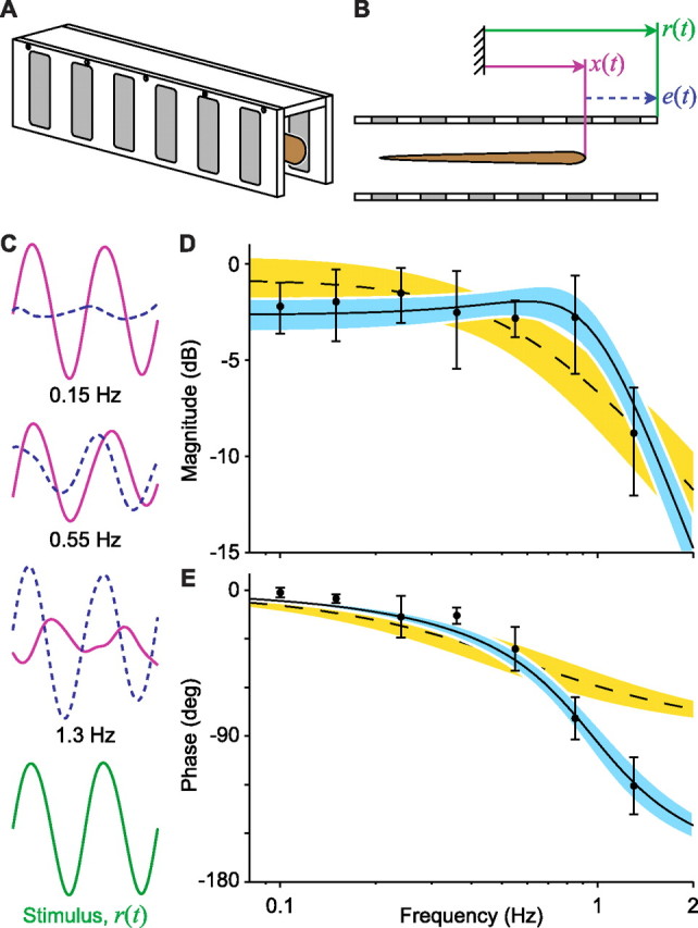
Identifying the whole-animal transfer function for longitudinal tracking behavior in Eigenmannia. A, The fish (brown) maintains its position within a rectangular tube. This refuge has a clear polycarbonate top and white plastic sides with ceramic-filled windows (gray). B, Schematic view of the video data captured using a camera positioned above the fish. Three values are the position of the fish [x(t), purple lines], the position of the refuge [r(t), green lines], and the relative difference between the fish and the refuge [e(t), dashed blue line]. C, Tracking data from a fish (stimulus amplitude, 0.5 cm). The height of each trace is scaled identically; the width of each trace is scaled to show two stimulus cycles (bottom; green) at three rates of motion (labeled). The amplitude of fish movements, x(t), decreased with increasing stimulus frequency with increasing phase lag. D, Bode amplitude. E, Bode phase plots for stimulus rates from 0.1–1.3 Hz. Error bars indicate the SD (N = 4 fish). The dashed curve indicates the first-order model (rejected), and the gold region indicates 95% confidence intervals for this model. The solid curve indicates the second-order model, and the blue region indicates 95% confidence intervals for this model.

Experimental trials consisted of moving the refuge sinusoidally at a particular amplitude (range, 0.5–4 cm) and frequency (range, 0.01–2 Hz). In addition, we ran a small number of 0.1–2 Hz chirp signals with amplitudes of 2–4 cm. There was typically 1 min pause between trials, and the order of the trials (different amplitude/frequency combinations) was randomized. Trials were typically conducted for <1 h/d over a period of 2 or 3 d.

A video camera (320 × 240 resolution, 30.0 Hz frame rate) was placed above the refuge within the armature used to move the refuge to include an overhead view of length of the refuge. Both the silhouette of the fish and a black transverse line placed below the tank were visible in the video field. Data were collected using a video capture system. Parallax was measured in the system, and the requisite compensation was made before data analysis.

The videos were imported into Matlab (MathWorks, Natick, MA), and the position of the fish and the position of the transverse line on the bottom of the tank were extracted in each frame. For each trial, we extracted the refuge position r(t), fish position x(t), and tracking error e(t) = r(t) − x(t) (Fig. 1C). These data were used to compute the gain and phase relationships (Fig. 1D,E).

Behavioral modeling.

We fit linear transfer function models between r(t) and x(t) of the following form:

for n = 1, 2, 3. In the second-order case, the model is rewritten as follows.

where ζ is the damping coefficient, ω_n is the undamped natural frequency, and A is the DC (zero frequency) gain.

Using the nlinfit command in Matlab, we fit the parameters A, a₁, a₂, and a₃ using Gauss-Newton nonlinear least-squares optimization to minimize the error between the model-predicted and observed gain and phase at each frequency for the lowest amplitude trial for each fish. The gain was scaled by a factor of 100, and the phase was measured in degrees so that they would have nearly equal weight over the range of magnitudes and phases observed.

The smooth-pursuit open-loop models of locomotion we used were a first-order kinematic and second-order mechanical model. The kinematic model simply states that the fish velocity is controlled directly by a locomotion “subsystem,” namely ẋ = u, where u is the locomotor control input. This hypothesis states that the transfer function from control input u(t) to fish position x(t) is given by the following:

Our mechanical model states that the fish acceleration is controlled directly according to Newton's second law, namely M ẍ = u + f_drag, where f_drag represents drag forces. A quasi-static model of drag predicts a drag force given by the following:

where ρ is the density of water, A is a characteristic area (in this case, the surface area of the fish), and C_D is the Reynolds-number-dependent drag coefficient (Fox et al., 2004). The characteristic length, L, is taken as the rostral–caudal length of the fish, and the Reynold's number is given byR_e = L v/ξ, where ξ is the kinematic viscosity of water. It follows from quasi-static fluid mechanical theory that for these knifefish, the drag results from laminar flow over a flat plate, namely C_D ∼ (R_e)^0.5 (Fox et al., 2004), and Blake (1983) experimentally confirmed that the drag coefficient for knifefish of similar sizes was consistent with this model. Under these conditions, the quasi-static drag is approximately the following:

where C will differ slightly for each animal. The linearization of the drag force is zero. Moreover, for the fish sizes (mean length, 12.5 cm; SD = 2.4 cm), and refuge motions (0.5 cm amplitude, 0.01–2.0 Hz) used for model fitting, one can bound the drag forces; drag forces are approximately one-tenth of acceleration forces. Therefore, we neglect the drag forces, as in Colgate and Lynch (2004). Thus, the mechanical system hypothesis is given by the transfer function, from control input u(t) to fish position x(t), namely the following:

Determining the sensorimotor transfer function.

Assume the sensory system (vision and electrolocation) measures fish positional error, e(t), relative to the environment, e.g., by integrating relative changes over large regions of the visual and electrosensory receptor arrays, as flies may do for optic flow (Humbert et al., 2005). Our goal is to determine the sensorimotor transformation, C(s), shown in the feedback control diagram in Figure 2A. Given G(s) and the (a priori unknown) sensorimotor transformation C(s), the closed-loop transfer function H(s) is as follows:

The coefficient A arises because mechanosensory lateral line, vestibular and other sensorimotor pathways not directly stimulated by the motion of the shuttle may attenuate (A < 1) the closed-loop response to shuttle motion. For the tracking behavior, we fit H(s) experimentally and compute C(s) from Equation 7 under differing assumptions about G(s) (see Eq. 3, 6).

Figure 2.

Closed-loop model of tracking behavior. A, Block diagram of the closed-loop control system including a model of locomotor dynamics and a neural multisensory controller, C(s). The locomotor dynamics can be modeled either using kinematics alone, 1/s (green), or using a model that includes mechanics, 1/Ms² (purple). B, Models of the C(s) filter; magnitude (in decibels) against frequency (in hertz). Kinematic locomotor plant predicts that C(s) is a low-pass filter (dotted green line); mechanical locomotor plant predicts that C(s) is a high-pass filter (dashed purple line). Tuning curves (blue lines; vector strength in decibels plotted against frequency) from ELL pyramidal neurons obtained under local (squares) and global (triangles) stimulus geometries (data from Chacron et al., 2003) match the high-pass filter prediction. All curves and data points are normalized to 0 dB.

Results

Tracking behavior

Tracking performance was measured for N = 7 fish, body length 12.5 cm (mean, SD = 2.4 cm), over a range of biologically salient frequencies (up to 2 Hz) and amplitudes (up to 4 cm, approximately one-third of body length). For each trial, the input refuge position r(t), output fish position x(t), and tracking error e(t) = r(t) − x(t) were measured (Fig. 1C), and the resulting gain and phase relationships were computed (Fig. 1D,E). For all fish, the tracking phase lag typically exceeded 90° for stimulus frequencies >1 Hz and always exceeded 90° at the highest frequency tested, 2 Hz. These phase lags can potentially be explained by second-order but not first-order linear dynamics.

Unlike the tracking phase, the relative tracking magnitude varied systematically with increasing stimulus amplitude. The relative tracking magnitude for stimulus frequencies >0.5 Hz was increasingly attenuated at stimulus amplitudes >1.0 cm. That is, the nonlinear attenuation was only apparent for stimuli that were both high frequency (>0.5 Hz) and high amplitude (>1.0 cm). This decrease of 3.7 dB cm⁻¹ (mean, SD = 1.8; N = 7), averaged over all frequencies >0.5 Hz, was significant (p < 0.002, one-tailed t test). This sort of amplitude-dependent saturation has also been observed in smooth-pursuit eye movements (Buizza and Schmid, 1986). We simulated the dynamics and included drag forces consistent with Blake's (1983) observations (see Materials and Methods) and determined that drag forces might contribute slightly to the nonlinearity but cannot fully explain it.

For N = 4 fish, we ran the lowest amplitude experiments, 0.5 cm, in which we suspected the saturation nonlinearity would be negligible. Indeed, a linear model fits well (Fig. 1D,E). For these data, second-order models fit significantly better than first-order models for each fish (N = 4, p < 0.05, t test on highest-order coefficient); when all of the trials from all fish are pooled together and fit to a single model, the first-order model is strongly rejected (p < 0.001). Furthermore, using the same criterion, a third-order model does not significantly improve the fit over the second-order model (N = 4, p > 0.05), even when all of the data from these four fish are pooled together. The fish exhibit a closed-loop bandwidth of f_n = 1.049 Hz (mean, SD = 0.16; N = 4), where f_n = ω_n/(2π) (see Materials and Methods). The DC gain is A = 0.73 (mean, SD = 0.09; N = 4), and the damping coefficient is ζ = 0.56 (mean, SD = 0.05; N = 4). Figure 1, D and E, shows the first- and second-order models and their confidence intervals with all four fish pooled together.

Neural control models

How does the nervous system of Eigenmannia transform sensory information into motor commands to achieve the observed second-order locomotor performance? We derived a model for the sensory transformation within a closed-loop system (Fig. 2A). This closed-loop system includes both sensory dynamics and locomotor dynamics. Determining the sensory dynamics requires a model for the locomotor dynamics (see Materials and Methods).

We tested the three lowest-order models for G(s). These models of locomotor dynamics include a zeroth-order saccadic model and two higher-order smooth-pursuit models: a first-order kinematic model and a second-order Newtonian model. A zeroth-order saccadic model describes jumps in position in response to sensory stimuli (Gilbert, 1997; Tammero and Dickinson, 2002; Tammero et al., 2004). This model was rejected for the Eigenmannia tracking behavior by inspection of the data: the animals clearly engage in smooth pursuit, not saccadic jumps.

A first-order kinematic model describes smooth motion in which the motor system generates velocities. This model of locomotor dynamics, when in closed loop (Fig. 2A), requires that the neural controller generate a velocity command to the motor plant. The power of these kinematic approaches, which are commonly used in the description of sensory-mediated locomotion (Collett et al., 1998; Srinivasan et al., 2000; Barron and Srinivasan, 2006; Ghose and Moss, 2006), is that they reduce task-level control of locomotion to simple kinematic movement, enabling one to find direct correlations between salient sensor readings and animal motion.

Here, the kinematic model of fish locomotion is a simple transfer function of the form G(s) = 1/s (see Materials and Methods) that relates the velocity command to fish position. Using the kinematic model, and given the fact that the closed-loop dynamics were found experimentally to be a damped harmonic oscillator, the algebraic solution (see Materials and Methods) for the neural controller C(s) is a first-order low-pass filter (Fig. 2B) of the following form:

The cutoff frequency is p/(2π) = 1.17 Hz (mean, SD = 0.26; N = 4).

A second-order model that includes mechanics describes smooth motion in which the motor system generates forces. In this model, forces produce motion according to Newton's second law. This Newtonian model requires that the neural controller generate a force command to the motor plant. For Eigenmannia, the second-order locomotion model incorporates the mechanical properties, namely inertia, of the fish. The fish must accelerate itself through a fluid, and thus, from Newton's second law, we have a mechanical plant with transfer function of the form G(s) = 1/(Ms²) (see Materials and Methods). The mass M includes the fish mass plus the added mass of the surrounding fluid (Colgate and Lynch, 2004).

Using the mechanics-based model and given that the closed-loop dynamics were found to be a damped harmonic oscillator, the algebraic solution (see Materials and Methods) for the neural controller C(s) is a first-order high-pass filter (Fig. 2B) of the following form:

This filter levels off above the cutoff frequency, which again is p/(2π) = 1.17 Hz (mean, SD = 0.26; N = 4).

Evaluation of the kinematic and mechanical models

The high-pass filter predicted by the mechanical model is categorically different from the low-pass filter predicted by the kinematic model. We evaluated these distinct neural control predictions in two ways. First, we looked for neural correlates of both control models in the electrosensory system. A neural correlate of the high-pass filtering regime occurs in p-type tuberous electrosensory afferents in Gymnotiform fishes and in pyramidal cells in the electrosensory lateral line lobe (ELL). Electrosensory responses in both of these systems exhibit high-pass filtering at frequencies <10 Hz (Bastian, 1986; Shumway, 1989). These responses, which occur in both local and global stimulation regimes (Chacron et al., 2003), appear to closely match the high-pass prediction from the mechanics-based double-integrator model (Fig. 2B). The majority of electrosensory midbrain (torus semicircularis) neurons exhibit bandpass responses in the range of 1–30 Hz, which is also consistent with the high-pass controller prediction C(s), <10 Hz (Rose and Fortune, 1999).

Second, we evaluated the stability and performance of the two controllers in a closed-loop simulation of fish swimming. This closed-loop simulation included a second-order Newtonian model of locomotor dynamics (Colgate and Lynch, 2004) (Fig. 3). The low-pass controller, when placed in closed loop with the Newtonian mechanical system, predicts poor tracking performance and is in fact unstable (some system poles are in the open right-half plane, which implies that the tracking error grows exponentially with time). In contrast, the high-pass controller, when placed in closed loop with the Newtonian mechanical system, is not only stable, but also closely matches the performance of the fish to a novel chirp stimulus (Fig. 3). That the stimulus response characteristics of the high-pass controller to a novel stimulus matches model predictions strongly supports the high-pass neural controller hypothesis.

Figure 3.

Stability and performance of the low-pass and high-pass controllers. Plots of the position of the fish over time are shown. The blue curve indicates the response of a fish to the novel increasing frequency stimulus: a frequency chirp. The dotted green curve indicates the unstable performance of the closed-loop model with a low-pass controller. The dashed purple curve demonstrates that the performance of the closed-loop model with a high-pass controller is similar to actual fish performance. Calibration: 1 s, 1 cm.

Why is the failure of the low-pass controller in the Newtonian closed-loop model important? Indeed, if one places this low-pass controller in a closed-loop model that neglects Newtonian mechanics, namely using a kinematic locomotion model, it exactly matches the performance of the high-pass controller in a closed-loop model that includes Newtonian mechanics shown in Figure 3. That is, the low-pass controller works well within a model that violates a fundamental physical reality, that the fish has mass. Critically, based on first principles, we know that the animal locomotor system must obey second-order Newtonian mechanics, and therefore a kinematic model alone of animal movement is insufficient. In this way, our result elucidates an important danger in the analysis of sensor-driven locomotor behavior: assuming a kinematics-based model in the context of nontrivial mechanics can lead to categorically incorrect predictions of sensory processing.

Discussion

We examined the processing features of a neural controller for locomotion using a combination of behavioral measurements and models. In an ideally suited behavioral model, Eigenmannia follow the longitudinal movement of a refuge by swimming back and forth to maintain position within the refuge. By measuring the performance of fish to a range of frequencies and amplitudes of sinusoidal stimuli, we found that performance is best at the lowest frequencies and has a bandwidth of ∼1 Hz. Phase lags were always >90° at the highest stimulus frequencies.

A model of the neural controller for this behavior that relies on kinematics alone predicts that the nervous system must implement a low-pass filter for stable control, whereas the model that includes mechanics predicts a high-pass filter. The high-pass filter matches the filtering properties of neurons in electrosensory systems and also leads to stable control in a closed-loop model of the behavior. Furthermore, the low-pass filter is unstable in a closed-loop model incorporating Newtonian mechanics.

Kinematic and mechanical analyses of behavior

Notwithstanding the critical role of mechanics highlighted by the results, kinematic analyses remain an important first step in the decoding of sensory systems. Kinematic analyses reveal salient features in the environment for the control of locomotion. An important feature in tracking behavior of Eigenmannia is that the steady-state kinematics are trivial: the fish maintains its position relative to a moving refuge. Indeed, it is this feature that makes tracking in Eigenmannia an ideal system for studying the controller dynamics.

In many systems, however, the sensory goal itself is unknown and must be discovered through kinematic analyses (Srinivasan et al., 1996; Okada and Toh, 2000; Srinivasan et al., 2000; Ghose and Moss, 2006). These analyses can be extended to make predictions about neural control systems using the same approach described above. Our data strongly suggest, however, that the use of kinematics alone is insufficient for the analysis of neural control of behavior. In addition to kinematic data, two additional ingredients are necessary to achieve accurate models for neural control: a set of sensorimotor perturbations (Bohm, 1995; Srinivasan et al., 1996) and a template model of the locomotor mechanics (Full and Koditschek, 1999).

Implications for sensory processing

In weakly electric fish such as Eigenmannia, locomotion simultaneously activates visual, electrosensory, and mechanical sensory systems. A previous report suggests that fish rely on both visual and electrosensory information, but not mechanosensory information, for refuge tracking (Rose and Canfield, 1993a). For this report, we focus on electrosensory processing because, unlike vision, the electrosensory feedback signal is directly linked to body motion and not confounded by ocular movements. Furthermore, there is a large body of quantitative analyses of neural processing in the electrosensory system of these fish (Rose and Fortune, 1999; Fortune, 2006), which we used to evaluate the control model C(s).

Recent work in electroreception has identified two spatiotemporal domains of sensory signals that match two distinct behaviors, prey capture and social signaling (MacIver et al., 2001; Chacron et al., 2003; Fortune et al., 2006). Prey capture involves a localized stimulus on the sensory array, whereas social signaling generates synchronous activation of the entire sensory array. These signals are thus described as “local” and “global,” respectively. A neural correlate of these two behavioral domains (local prey capture and global social communication) occurs in the dynamic receptive field properties of ELL neurons: centered at ∼10 Hz, local stimuli elicit low-pass responses, whereas global stimuli elicit high-pass responses (Chacron et al., 2003).

In tracking behavior, fish minimize local and global electroreceptive flow, which in turn minimizes the activation of the electrosensory system. Not surprisingly, therefore, for the range of stimulus frequencies (<2 Hz) involved in tracking behavior, the receptive field properties appear to agree with the high-pass controller model for both local and global stimuli (Fig. 2B). In contrast, prey capture requires localized flow across the receptor array, which results in strong local activation of receptors at ∼10 Hz (MacIver et al., 2001). These two locomotor tasks, therefore, have starkly different sensory goals and spatiotemporal filtering requirements. This suggests that there are actually three distinct behaviors that define three distinct spatiotemporal sensory regimes: social communication (global, >10 Hz), prey capture (local, ∼10 Hz), and locomotor tracking (local and global, <10 Hz).

Tracking is a form of image stabilization; image stabilization via motor compensation is ubiquitous across animal taxa. Refuge tracking in weakly electric knifefish is ideally suited to investigate sensorimotor control via image stabilization because (1) the locomotor system is bidirectionally symmetric for this behavior, and (2) fish position is directly linked to the electrosensory image. These simplifications in mechanics and sensing result from the unique form of propulsion, a ventral undulatory ribbon fin, used by these fish, and by the features of electrosensation (Fortune, 2006). Nevertheless, these data may be broadly relevant because many studies have shown that the mechanics of locomotion are similar across a wide range of animal morphologies, sizes, and locomotor mechanisms (Blickhan and Full, 1993; Dickinson et al., 2000; Holmes et al., 2006). Within this context, therefore, these data may suggest that similar sensory filtering (high-pass filtering in the low-frequency locomotor regime) is used for locomotor control in many other animal species. That the key temporal processing features of the underlying neural control of locomotion first appear at the level of sensory afferents and their targets in the CNS is not surprising: most animal locomotion generates widespread activation of sensory systems.

References

- Barron A, Srinivasan M. Visual regulation of ground speed and headwind compensation in freely flying honey bees (Apis mellifera L.) J Exp Biol. 2006;209:978–984. doi: 10.1242/jeb.02085. [DOI] [PubMed] [Google Scholar]
- Bastian J. Vision and electroreception: integration of sensory information in the optic tectum of the weakly electric fish Apteronotus albifrons. J Comp Physiol A Neuroethol Sens Neural Behav Physiol. 1982;147:287–297. [Google Scholar]
- Bastian J. Electrolocation: behavior, anatomy, and physiology. In: Bullock TH, Heiligenberg W, editors. Electroreception. New York: Wiley; 1986. pp. 577–612. [Google Scholar]
- Blake RW. Swimming in the electric eels and knifefishes. Can J Zool. 1983;61:1432–1441. [Google Scholar]
- Blickhan R, Full RJ. Similarity in multilegged locomotion: bouncing like a monopode. J Comp Physiol A Neuroethol Sens Neural Behav Physiol. 1993;173:509–517. [Google Scholar]
- Bohm H. Dynamic properties of orientation to turbulent air current by walking carrion beetles. J Exp Biol. 1995;198:1995–2005. doi: 10.1242/jeb.198.9.1995. [DOI] [PubMed] [Google Scholar]
- Buizza A, Schmid R. Velocity characteristics of smooth pursuit eye movements to different patterns of target motion. Exp Brain Res. 1986;63:395–401. doi: 10.1007/BF00236858. [DOI] [PubMed] [Google Scholar]
- Chacron MJ, Doiron B, Maler L, Longtin A, Bastian J. Non-classical receptive field mediates switch in a sensory neuron's frequency tuning. Nature. 2003;423:77–81. doi: 10.1038/nature01590. [DOI] [PubMed] [Google Scholar]
- Colgate J, Lynch KM. Mechanics and control of swimming: a review. IEEE J Oceanic Eng. 2004;29:660–673. [Google Scholar]
- Collett M, Collett TS, Bisch S, Wehner R. Local and global vectors in desert ant navigation. Nature. 1998;394:269–272. [Google Scholar]
- Cowan NJ, Lee J, Full RJ. Task-level control of rapid wall following in the American cockroach. J Exp Biol. 2006;209:1617–1629. doi: 10.1242/jeb.02166. [DOI] [PubMed] [Google Scholar]
- Dickinson MH, Farley CT, Full RJ, Koehl MA, Kram R, Lehman S. How animals move: an integrative view. Science. 2000;288:100–106. doi: 10.1126/science.288.5463.100. [DOI] [PubMed] [Google Scholar]
- Fortune ES. The decoding of electrosensory systems. Curr Opin Neurobiol. 2006;16:474–480. doi: 10.1016/j.conb.2006.06.006. [DOI] [PubMed] [Google Scholar]
- Fortune ES, Rose GJ, Kawasaki M. Encoding and processing biologically relevant temporal information in electrosensory systems. J Comp Physiol A Neuroethol Sens Neural Behav Physiol. 2006;192:625–635. doi: 10.1007/s00359-006-0102-0. [DOI] [PubMed] [Google Scholar]
- Fox R, McDonald A, Pritchard P. Ed 6. New York: Wiley; 2004. Introduction to fluid mechanics. [Google Scholar]
- Full RJ, Koditschek DE. Templates and anchors: neuromechanical hypotheses of legged locomotion on land. J Exp Biol. 1999;202:3325–3332. doi: 10.1242/jeb.202.23.3325. [DOI] [PubMed] [Google Scholar]
- Ghose K, Moss CF. Steering by hearing: a bat's acoustic gaze is linked to its flight motor output by a delayed, adaptive linear law. J Neurosci. 2006;26:1704–1710. doi: 10.1523/JNEUROSCI.4315-05.2006. [DOI] [PMC free article] [PubMed] [Google Scholar]
- Gilbert J. Visual control of cursorial prey pursuit by tiger beetles (Cicindelidae) J Comp Physiol A Neuroethol Sens Neural Behav Physiol. 1997;181:217–230. [Google Scholar]
- Holmes P, Full RJ, Koditschek D, Guckenheimer J. Dynamics of legged locomotion: models, analyses, and challenges. Sci Am Rev. 2006;48:207–304. [Google Scholar]
- Humbert JS, Murray RM, Dickinson MH. Pitch-altitude control and terrain following based on bio-inspired visuomotor convergence. Paper presented at AIAA Conference on Guidance, Navigation and Control; august; San Francisco, CA. 2005. [Google Scholar]
- MacIver MA, Sharabash NM, Nelson ME. Prey-capture behavior in gymnotid electric fish: motion analysis and effects of water conductivity. J Exp Biol. 2001;204:543–557. doi: 10.1242/jeb.204.3.543. [DOI] [PubMed] [Google Scholar]
- Okada J, Toh Y. The role of antennal hair plates in object-guided tactile orientation of the cockroach (Periplaneta americana) J Comp Physiol A Neuroethol Sens Neural Behav Physiol. 2000;186:849–857. doi: 10.1007/s003590000137. [DOI] [PubMed] [Google Scholar]
- Rose GJ, Canfield JG. Longitudinal tracking responses of the weakly electric fish, Sternopygus. J Comp Physiol A Neuroethol Sens Neural Behav Physiol. 1993a;171:791–798. [Google Scholar]
- Rose GJ, Canfield JG. Longitudinal tracking responses of Eigenmannia and Sternopygus. J Comp Physiol A Neuroethol Sens Neural Behav Physiol. 1993b;173:698–700. [Google Scholar]
- Rose GJ, Fortune ES. Mechanisms for generating temporal filters in the electrosensory system. J Exp Biol. 1999;202:1281–1289. doi: 10.1242/jeb.202.10.1281. [DOI] [PubMed] [Google Scholar]
- Shumway CA. Multiple electrosensory maps in the medulla of weakly electric gymnotiform fish. I. Physiological differences. J Neurosci. 1989;9:4388–4399. doi: 10.1523/JNEUROSCI.09-12-04388.1989. [DOI] [PMC free article] [PubMed] [Google Scholar]
- Srinivasan M, Zhang S, Lehrer M, Collett T. Honeybee navigation en route to the goal: visual flight control and odometry. J Exp Biol. 1996;199:237–244. doi: 10.1242/jeb.199.1.237. [DOI] [PubMed] [Google Scholar]
- Srinivasan M, Zhang S, Chahl J, Barth E, Venkatesh S. How honeybees make grazing landings on flat surfaces. Biol Cybern. 2000;83:171–183. doi: 10.1007/s004220000162. [DOI] [PubMed] [Google Scholar]
- Tammero LF, Dickinson MH. The influence of visual landscape on the free flight behavior of the fruit fly Drosophila melanogaster. J Exp Biol. 2002;205:327–343. doi: 10.1242/jeb.205.3.327. [DOI] [PubMed] [Google Scholar]
- Tammero LF, Frye MA, Dickinson MH. Spatial organization of visuomotor reflexes in Drosophila. J Exp Biol. 2004;207:113–122. doi: 10.1242/jeb.00724. [DOI] [PubMed] [Google Scholar]