Topographic Organization in and near Human Visual Area V4

Abstract

The existence and location of a human counterpart of macaque visual area V4 are disputed. To resolve this issue, we used functional magnetic resonance imaging to obtain topographic maps from human subjects, using visual stimuli and tasks designed to maximize accuracy of topographic maps of the fovea and parafovea and to measure the effects of attention on topographic maps. We identified multiple topographic transitions, each clearly visible in ≥75% of the maps, that we interpret as boundaries of distinct cortical regions. We call two of these regions dorsal V4 and ventral V4 (together comprising human area V4) because they share several defining characteristics with the macaque regions V4d and V4v (which together comprise macaque area V4). Ventral V4 is adjacent to V3v, and dorsal V4 is adjacent to parafoveal V3d. Ventral V4 and dorsal V4 meet in the foveal confluence shared by V1, V2, and V3. Ventral V4 and dorsal V4 represent complementary regions of the visual field, because ventral V4 represents the upper field and a subregion of the lower field, whereas dorsal V4 represents lower-field locations that are not represented by ventral V4. Finally, attentional modulation of spatial tuning is similar across dorsal and ventral V4, but attention has a smaller effect in V3d and V3v and a larger effect in a neighboring lateral occipital region.

Introduction

A first aim for researchers studying the visual system is to identify the components, or visual areas (Felleman and Van Essen, 1991; Crick and Jones, 1993), of the system, each of which contributes uniquely to a constellation of functions (Van Essen and Gallant, 1994). One reliable criterion for identifying early and intermediate visual areas is topographic organization (Kaas, 2004; Van Essen, 2004). In addition, topographic organization is itself a suitable substrate for many spatiotemporal neural computations (Kaas, 1997).

Several laboratories have mapped visual topography in human occipital cortex (Sereno et al., 1995; DeYoe et al., 1996; Tootell et al., 1997; Hadjikhani et al., 1998; Smith et al., 1998; Press et al., 2001; Tootell and Hadjikhani, 2001; Huk et al., 2002; Wade et al., 2002; Brewer et al., 2005; Tyler et al., 2005; Wandell et al., 2005; Hagler and Sereno, 2006; Larsson and Heeger, 2006; Swisher et al., 2007). These studies have shown that the topographic organizations of visual areas V1, V2, V3, and V3A are similar in humans and macaques, consistent with the notion that some functional and developmental aspects of these areas are conserved across species. However, the organization of human cortex potentially homologous to macaque V4 is still disputed. There are currently two principal organizational schemes depicting human V4 topography (Tootell and Hadjikhani, 2001; Wade et al., 2002), but these are mutually contradictory.

A consensus on human V4 will further studies of human form and color vision, because much of our understanding of intermediate form and color vision comes from studies of macaque dorsal V4 (Ungerleider and Mishkin, 1982; Desimone and Schein, 1987; Gallant et al., 1993, 1996; Kobatake and Tanaka, 1994; Pasupathy and Connor, 1999). Furthermore, the topography of visual areas neighboring V4 depend on the boundaries of V4, so a consensus on human V4 will also help resolve controversies surrounding nearby visual areas (Hadjikhani and Tootell, 1998; Tootell and Hadjikhani, 2001; Wade et al., 2002; Tyler et al., 2005; Brewer et al., 2005; Larsson and Heeger, 2006).

We performed topographic mapping experiments designed to identify the human counterpart of macaque area V4, if one exists. Our data show that topographic organization immediately anterior to human V3 is consistent with multiple defining characteristics of macaque V4, as observed by Gattass et al. (1988) (Fig. 1). First, in both species a dorsal region adjacent to parafoveal V3d represents one part of the lower field. Second, in both species a ventral region adjacent to V3v represents a different part of the lower field plus the upper field. Third, in both species the dorsal and ventral regions meet in the foveal confluence shared with V1, V2, and V3.

Figure 1.

Topography of human V1, V2, and V3 and macaque V4. Steps of transformations from the visual world and the cortical surface are shown as successive columns. The left column shows the visual field, with the upper field above and lower field below. Before visual information reaches the cortex, it is split into two halves (scissor icon) along the vertical meridian. The second column shows one visual hemifield using the same color legend as the actual fMRI maps (see remaining figures). In this and subsequent columns, the vertical cut is highlighted with circles. The third column shows how the visual hemifield is transformed further before reaching the cortical surface: the lower field is represented on top (i.e., dorsally), and the upper field is represented on the bottom (i.e., ventrally). The arrows link the same visual field locations before and after the transformation (purple-to-purple, blue-to-blue). The fourth column provides a rough illustration of how the visual field transformation might be distorted on the cortical surface. V1, Allman and Kaas (1974) named this type of transformation (a simple continuous map) a first-order transformation of the visual hemifield. V2, This transformation resembles V1 in most respects but includes an additional cut that does not follow the vertical meridian (additional scissors icon and stars). The off-vertical cut splits apart the dorsal and ventral portions (top and bottom, two rightmost panels). Allman and Kaas (1974) named this type of split transformation second order. The V2 and V1 transformations also differ in that V2 is not mirror reversed (upper-to-lower angles run roughly counterclockwise in the V2 panel but in the opposite direction in V1). Visual field coverage in V2d and V2v are complementary (i.e., each region represents part of the hemifield that the other does not). V3, The transformation resembles that of V2, except that it is mirror reversed. V4, The macaque V4 visual field transformation resembles that of V2, except that the off-vertical visual field cut is not always along the horizontal. In some individual macaques, it runs through the lower field, such that both V4d and V4v include some lower-field representation. However, visual field coverage in V4d and V4v (like that in V2d and V2v) are still complementary. V4 (like V2) is a non-mirror-reversed second-order transformation. The top black and white V4 panels are adapted from Figure 22 of Gattass et al. (1988).

Materials and Methods

Data acquisition

All procedures were approved by the University of California (UC) Berkeley Committee for the Protection of Human Subjects. Eight subjects were included in a study that mapped foveal/parafoveal visual space, and six subjects were in a study mapping parafoveal/peripheral visual space. Five of these subjects participated in both studies. All subjects had normal or corrected-to-normal visual acuity.

Blood oxygenation level-dependent (BOLD) functional data were collected with a whole-head volume radiofrequency (RF) coil (subjects 1, 2, and 5; peripheral-attention maps) or a curvilinear quadrature transmit/receive surface RF coil (all other maps) on a 4T Varian (Palo Alto, CA) INOVA scanner at UC Berkeley.

The foveal study used a one-shot gradient-echo echo planar imaging (EPI) sequence [repetition time (TR), 1 s; echo time (TE), 28 ms]. Twenty-four (in subjects 1–4) or 16 (in subjects 5–8) 2 mm coronal slices of the occipital lobe were acquired; the in-plane matrix size was 64 × 64, and the nominal resolution was 2 × 2 mm. The peripheral-attention study used a two-shot gradient-echo EPI sequence (TR, 1 s per shot; TE, 29 ms). Sixteen 3 mm coronal slices of the occipital lobe were acquired; the in-plane matrix size was 64 × 64, and the nominal resolution was 3 × 3 mm.

T1-weighted images were acquired in-plane with the functional images to permit coregistration to high-resolution anatomical images. High-resolution anatomical images were collected on a 1.5T Philips Eclipse scanner at the Veterans Affairs Hospital in Martinez, California. For each subject, two MP-RAGE (magnetization prepared rapid gradient echo) three-dimensional (3D) anatomical datasets were acquired, coregistered, and averaged. The matrix size was 256 × 212 × 256, and the resolution was 0.9375 × 1.3 × 0.9375 mm. Any differences between the Martinez 3D anatomical images and the Berkeley in-plane coronal anatomical images were minimal (<0.5 mm at all points).

Visual stimuli were backprojected onto a translucent screen by a liquid crystal display projector. An obliquely positioned mirror allowed the supine subjects to view a virtual image of the screen. A rigid plastic occluder prevented the appearance of a double image in the lower periphery of the visual field. Head motion was minimized with foam padding.

Matlab (versions 6.0 and 7.0; Mathworks, Natick, MA) functions written by the authors were used to generate all stimuli and to perform all data analyses and data visualization, unless indicated otherwise. Matlab functions from the Psychophysics Toolbox (Brainard, 1997; Pelli, 1997) were used to present stimuli in the scanner.

Stimuli and tasks

Foveal/parafoveal maps and foveal attention.

Angle stimuli (Fig. 2) consisted of a 90° wedge rotating continuously around a 0.1° fixation point with a period of 36 s. The wedge was filled with a high-contrast, flickering, black-and-white radial checkerboard texture that also rotated continuously, at the same speed and direction as the wedge. The space inside the circle swept out by the wedge but outside the wedge itself was filled by the same checkerboard texture at very low contrast. The low-contrast texture also rotated continuously, at the same speed and direction as the wedge.

Figure 2.

Stimuli and tasks. A, Foveal angle-mapping stimuli. A wedge, 90° in angular width and 5.1° in radial eccentricity, rotated around a fixation point in continuous motion. The texture within the wedge was a high (100%)-contrast, black-and-white radial checkerboard, scaled exponentially. The texture inside the circle swept out by the wedge (but outside the wedge itself) was the same checkerboard at low (2%) contrast. The screen outside this circle was isoluminant gray. Both the high- and the low-contrast textures rotated around the fixation point at the same speed as the wedge (one period was 36 s). B, Foveal eccentricity-mapping stimuli. A ring (the thickness of which was scaled logarithmically with distance from fixation) expanded or contracted around the fixation point in discrete jumps. The maximal eccentricity subtended by the ring was 5.1 radial degrees. At all positions, the ring was as wide as two checks. C, Peripheral angle-mapping stimuli. The m-sequence controlling wedge presentation was 255 frames long; onset time is indicated above each image. The figure suggests static images, but the phase of each grating was varied systematically to produce a dynamic animation. D, Peripheral eccentricity-mapping stimuli. The same m-sequence as in C controlled the presentation of four individual rings, of thickness scaled with distance from fixation. The underlying grating texture and timing parameters were the same as those used for the wedges. E, Attention task. The mapping experiment was repeated a multiple of eight times (wedge, shown here) or four times (ring). Each time, the subject fixated a central cross and covertly attended the texture in a different wedge or ring. F, Control task. Subjects reported subtle changes in luminance in a small (0.3°) circle around the fixation cross. The stimuli were identical to those used in the attention task.

Our early pilot datasets, which did not use the low-contrast background texture, often contained an artifact that suggested subjects were unintentionally tracking the innermost portion of the rotating wedge. Specifically, an artifactual stripe of apparent lower-field spatial tuning appeared just ventral to the cortical fovea, and an artifactual stripe of apparent upper-field spatial tuning appeared just dorsal to the cortical fovea. [Many examples of this familiar artifact exist in the functional magnetic resonance imaging (fMRI) literature. The one in Figure 6B from Tootell and Hadjikhani (2001) is helpful because hash marks overlay the data to illustrate explicitly where the estimated spatial tuning was likely caused by artifact.] The purpose of the background texture was to help subjects maintain better fixation at the central point. Adding the rotating low-contrast background effectively placed the fixation cross at the center, rather than the edge, of a perceptually coherent texture. When the low-contrast background was added to the wedge stimuli, the characteristic artifactual stripes disappeared from the angular maps.

Figure 6.

Complementary visual field coverage in dorsal and ventral V4. A, The V4 data from Figure 5 are divided into ventral V4 (top, purple), dorsal V4 (middle, green), and V4 as a whole (bottom, overlapping purple and green). Across subjects and hemispheres, the ventral V4 data consistently do not cover the parafoveal lower visual field, but the dorsal V4 data do, and area V4 data as a whole cover the entire stimulated visual field. B, Each numeral gives the number of hemispheres (of 12) in which the estimated spatial tuning of at least two surface vertices in ventral V4 (left) or dorsal V4 (right) was within the corresponding sector. The sectors are shown to scale; each is 1° of eccentricity by 30° of polar angle. C, The same information as in B is represented graphically. Two key observations are apparent. First, visual field coverage in dorsal V4 is complementary to visual field coverage in ventral V4 (compare similar observation in macaque V4 in Fig. 1). Second, the visual field cut that splits the dorsal and ventral portions is typically not along the horizontal meridian, as is the case in the more familiar areas V2 and V3. Instead, the visual field cut tends to occur at intermediate lower-field angles (compare macaque V4 in Fig. 1).

Eccentricity stimuli (Fig. 2) consisted of logarithmically scaled rings that expanded or contracted at 4.5 s intervals. During the 36 s period, the ring occupied one of eight distinct positions. The ring was filled by a high-contrast, static, black-and-white radial checkerboard, identical to the texture used inside the wedge. For consistency, the space outside the ring was filled by a low-contrast but perceptible black-and-white radial checkerboard texture identical to the texture used outside the wedge. Adding the low-contrast background texture did not alter the eccentricity maps. The distance between the fixation point and the maximum eccentricity covered by the high-contrast checkerboard was 5° (at 0.025° per pixel).

During data acquisition, the fixation point stochastically switched between red and blue every 500–2667 ms. Subjects pressed a button every time they detected that the fixation point turned blue. This task forced the subjects to maintain close fixation.

Each 3.6 min phase-encoded stimulus covered one of four conditions: wedge clockwise; wedge counterclockwise; ring expanding; ring contracting. In each scan session, the set of all four 3.6 min fMRI experiments was presented four times. Between sets, the subject rested while an in-plane anatomical reference image was acquired. The in-plane images allowed each set to be registered independently to the cortical surface. This step minimized potential contamination from small, cumulative changes in head position across the session.

Parafoveal/peripheral maps and parafoveal/peripheral attention.

Angle stimuli consisted of eight adjacent 45° wedges, and eccentricity stimuli consisted of four concentric rings (Fig. 2). Each wedge or ring turned ON (containing a texture described below) or OFF (isoluminant gray, like the background) over the course of the stimuli. The texture consisted of overlapping polar and hyperbolic non-Cartesian gratings (Gallant et al., 1993, 1996). Gratings were assigned random locations within the wedges or rings. The radii of the gratings were chosen so that the resulting stimulus approximated a 1/f² spatiotemporal power spectrum (each image contained n gratings of size a, 2n gratings of size a/2, 4n gratings of size a/4, etc.). The spatial phase of each grating was advanced slightly on each image frame to create dynamic stimuli (spiral gratings rotated clockwise or counterclockwise, hyperbolic gratings expanded or contracted). The color, spatial frequency, and apparent velocity of each grating were assigned randomly. The central 2° (1° radius) of visual angle was excluded from the wedges to minimize potential artifact from subtle eye movements. The distance between the fixation point and the maximal eccentricity covered by the dynamic texture was 18° (at 0.072° per pixel) for experiments involving the whole-head coil and 15.5° (at 0.062° per pixel) for experiments involving the surface coil.

This dynamic texture was not used for the foveal/parafoveal maps (section above) for two reasons. First, we were concerned that placing a dynamic texture adjacent to the fixation point might lead to fixation inaccuracy. Second, the use of a black-and-white flickering checkerboard for at least one set of topographic maps eliminated the possibility that differences between our conclusions and those of other laboratories might be attributable to stimulus texture.

A small central cross (0.25°) was present at all times and served as a fixation target. A faint white disk of the same radius as the fixation cross appeared in varying contrasts behind the cross; the disk was unobtrusive and did not overlap any of the attended regions. In a control task, subjects pressed a button when the disk was brighter than what the subjects perceived as average; the control data allowed us to verify that maps made by averaging data from different peripheral-attention conditions (see below) were comparable to maps made from data acquired while subjects performed an easy attention task at the fixation point.

In the attention task, subjects pressed a button when they detected target spirals (polar gratings) centered within the attended wedge or ring. Target spirals were defined by their size alone and could be of any color, polarity, phase, or spatial or temporal frequency. Targets were always large enough to be detectable at the maximum eccentricity of the attended region, and usually one or more target spirals were present whenever a given wedge or ring was ON. Before each run, a text instruction (e.g., “lower right wedge near the horizontal meridian”) indicated to the subject which wedge should be attended; data acquisition began only after the subject confirmed that s/he understood the instruction.

Subjects (two of them authors) were aware that the purpose of the detection task was simply to help them direct covert attention to a specific region of the visual field. It was made clear to all subjects that the most important part of the task was to maintain fixation, even at the potential expense of missing some targets. Data were acquired from eight subjects. The data from one subject were discarded because this subject's V1 topographic maps shifted across runs, indicating that the subject maintained poor fixation. The data from another were discarded because the signal-to-noise ratio fluctuated widely across runs, indicating that the subject's general arousal level varied greatly across conditions.

The temporal ON/OFF sequence for a given wedge or ring was controlled by a binary 8-bit m-sequence of length 2⁸ − 1 = 255. Each element of the sequence lasted for 4 s, so that a single experiment required 17 min of scan time. Although a 17 min scan is relatively long, maps from individual subjects were similar to maps from the same subjects produced with short 3.6 min phase-encoded stimuli. Between each 17 min experiment, subjects rested while an in-plane anatomical reference image was acquired. The in-plane images allowed us to register each set independently to the cortical surface. This process minimized potential contamination from small, cumulative changes in head position across the session.

Each scan session included four attention conditions, covering the complete left visual field, the complete right visual field, or the complete set of rings. Thus, multiple scan sessions were required to collect one complete dataset for one subject. To avoid potential order artifacts, we used a randomly generated order for the attention conditions in each scan session. To increase signal in experiments involving the volume coil, and to check for map stability over multiple days, wedge attention conditions were repeated four times in subject 1 and two times in subjects 2 and 5, and ring attention conditions were repeated three times in subject 1 and two times in subjects 2 and 5.

Motion localizer.

MT+ was localized in separate experiments in subjects who participated in the parafoveal/peripheral mapping study. Each 400 s localizer scan alternated between 10 s “motion” and 30 s “no-motion” blocks. During motion blocks, a set of randomly positioned white dots moved radially inward and outward, and during no-motion blocks, the randomly positioned white dots remained stationary. Subjects fixated on a central cross for the duration of the experiment. Mean signal levels during motion and no-motion blocks were compared via a t test. The results were consistent with previous reports (Tootell et al., 1995; Huk et al., 2002): motion blocks evoked significantly higher signal in parts of V1, V3A, and parietal cortex and in a cluster in/near the dorsal part of the inferior temporal sulcus, which we identified as MT+.

Preprocessing

Functional brain volumes were reconstructed to image space using software written by J. J. Ollinger at the Berkeley Brain Imaging Center (available at http://cirl.berkeley.edu). The software reduced Nyquist ghosts using a reference scan from the start of the time series; corrected the data for differences in slice acquisition times; and, for the two-shot data, linearly interpolated the brain volume images over time to 1 s per image. Images were inspected to verify an absence of excessive head motion using the motion detection/correction algorithm in SPM99 (http://www.fil.ion.ucl.ac.uk/spm/). Images were then linearly detrended and high-pass filtered at 1/60 Hz.

Volume-to-surface transformations

Reconstruction of the cortical surface and flattening were performed using SureFit and Caret [http://brainmap.wustl.edu/caret (Van Essen et al., 2001)]. We found that this package produced relatively accurate initial segmentations. Because of the small folds in the cortical surface, the thinness of the gray matter, and contrast variations in the anatomical images, substantial additional manual corrections were made to fully represent every sulcus and gyrus.

To visualize the topographic maps, in-plane anatomical images were coregistered to the 3D high-resolution anatomical image from which the cortical surface was reconstructed. In-house software was used to coregister the images. This software permits manual coregistration of images using affine transformations. Accuracy of coregistration was confirmed via visual inspection of all three slice orientations. Before using this software in the current study, we compared the transformation parameters given by our software to those given by the automatic and manual alignment functions in a commercial package. In the hands of experienced users, our software produced considerably more accurate transformation parameters; these were closely replicated by different users. The surfaces consisted of vertices generally separated by <1 mm. Voxel data from each fMRI run were linearly interpolated onto the vertices. Data from different runs were combined on a vertex-by-vertex basis, and statistical analyses were performed on a vertex-by-vertex basis.

Data analysis

Foveal/parafoveal maps.

For clockwise or counterclockwise wedge data, the phase of the Fourier component at the stimulus frequency (1/36 Hz) was calculated using the discrete Fourier transform. The two phases were then averaged, producing the phase associated with peak wedge tuning. The phase associated with peak ring tuning was calculated similarly with expanding and contracting ring data.

The phase-encoded wedge data (in units of seconds) were converted directly to polar angles in the visual field. This practice is routine in most phase-encoded topographic mapping studies (Press et al., 2001; Brewer et al., 2005). Recent validation studies from our laboratory (Kay et al., 2005) have confirmed that this conversion step produces reasonable estimates of polar angle in most voxels.

The phase-encoded ring data were left in units of seconds. This practice is routine in most phase-encoded topographic mapping studies (Press et al., 2001; Brewer et al., 2005). It is theoretically possible to convert the data from seconds to degrees of visual angle subtended, because there is a one-to-one relationship between phase and eccentricity. However, conversion would implicitly assume that voxels in every visual area respond with time courses of the same shape to expanding and contracting rings. To the best of our knowledge, this assumption has not been tested explicitly. In this study, therefore, we have followed common practice and left phase-encoded ring data in units of seconds.

The map data were thresholded by the SE of phase estimates across different scans (supplemental material, available at www.jneurosci.org). Estimates with a SE of ≥3 s of the 36 s period do not appear (i.e., are colored white) on the maps.

Visual field coverage plots.

Regions of interest (ROIs) were defined based on boundaries of topographic regions (see Results). The preferred angle and eccentricity values at each point within each ROI were then identified. Finally, each pair of angle and eccentricity values was projected back into retinal coordinates to obtain two-dimensional visual field coverage plots.

The final transformation assumes that two-dimensional spatial tuning estimates of angle/eccentricity combinations can be estimated accurately by combining independent measurements of angle and of eccentricity. A previous publication from our laboratory (Hansen et al., 2004a) validated this assumption in V1.

Parafoveal/peripheral-attention-modulated maps.

For the peripheral-attention data, reverse correlation was used to estimate the response of each voxel to all wedges and rings (Hansen et al., 2004a). The stimulus design matrix consisted of a baseline term and the ON/OFF state of each wedge or ring at different time lags. This matrix was used to obtain the ordinary least-squares estimate of the kernel of each voxel. To quantify the response of a voxel to a given wedge or ring, the kernel response between 3 and 5 s after stimulus onset was summed. We chose this lag window (associated with the rise and peak of the estimated hemodynamic responses) because we observed that time courses were more consistent across voxels in this window than at other lags.

Negative response amplitudes were discarded by setting them to zero. This conservative step allowed us to verify that our conclusions about topographic organization were based on true stimulus responsivity rather than on a potential artifact first noted by Sereno and Tootell (2005): visual stimuli can suppress BOLD signal in parts of cortex preferring nearby visual field locations, but periodic suppression is translated into false-positive spatial preference by the phase-encoding analysis. In practice, the maps of the regions described in this study were very similar before and after this step. (For more details on positive vs negative responses to stimuli, see supplemental material, available at www.jneurosci.org.)

Error bars and statistical significance were estimated using nonparametric jackknifing (Efron and Tibshirani, 1993). In jackknifing, the data are randomly divided into n disjoint subsets. Parameter estimates are obtained n times, each time excluding a different subset of the data. SEs are calculated based on the variance across the n parameter estimates.

A vector-averaging procedure was used to convert responses evoked by discrete wedges into a continuous-valued estimate of angle preference. Each vertex on the virtual cortical surface was assigned eight vectors, representing responses to each of the eight wedges. The angular value of the average of these eight vectors was plotted on the maps. Maps were constructed by averaging data from all attention conditions together. Thus, the maps reflect attention to stimuli in all parts of the stimulated visual field.

To create threshold values for the map data, the uncertainty of retinotopic angle tuning was used as a statistic in a randomization procedure. First, error bars on the actual response amplitude to each wedge were calculated. Then, a distribution of 200 randomized tuning values was obtained via resampling, and the 95% confidence interval on this distribution was calculated. The process was repeated for 200 randomized dummy amplitudes, producing a distribution of 95% confidence interval values that could have resulted if there were no angular tuning. The statistical significance (p value) of the actual confidence interval was calculated as the proportion of randomized confidence intervals that were narrower than the observed confidence interval.

A center-of-mass procedure was used to convert response amplitudes to discrete rings into continuous-valued estimate of eccentricity preference. The eccentricity tuning was calculated as

where a₁, a₂, a₃, a₄ are the response amplitudes to the four rings, and k₁, k₂, k₃, k₄ are the mean eccentricities of the four rings (mean eccentricities for the parafoveal/peripheral rings are 12.7, 5.1, 3.4, and 0.5° for datasets acquired in the volume coil and 10.6, 4.2, 2.8, and 0.4° for datasets acquired in the surface coil).

When a center of mass analysis is applied to a dataset containing only positive values, the analysis cannot produce results smaller than the minimum or larger than the maximum values. For example, in parts of peripheral V1, the largest ring elicited positive responses and other rings elicited no responses (or negative responses that were set to zero; see above), so the center of mass analysis assigns the mean eccentricity of the largest ring to the surface vertices. To take this bias into account, the color scale was designed so that eccentricities between the mean and maximum eccentricities of the largest ring all received the same purple color. As a rough assessment of overall bias, we compared maps from nonrectified BOLD data. Apart from regions that apparently represented eccentricities beyond the mean of the largest ring, the maps were very similar.

For each surface vertex, the statistical significance (p value) of an eccentricity tuning value was taken to be the minimum p value associated with any of the four rings. All p values were multiplied by 0.25 to compensate for multiple comparisons between four rings.

The lower-resolution 3 × 3 × 3 mm parafoveal/peripheral topographic maps, averaged across attention conditions (supplemental material, available at www.jneurosci.org), were in good agreement with the higher-resolution 2 × 2 × 2 mm foveal/parafoveal maps. Given the 3 × 3 × 3 and 2 × 2 × 2 maps for the same hemispheres, most of the boundary criteria (described in Results) appeared equally clearly in both. However, because dorsal V4 is a narrow region that extends a relatively short distance outside the foveal confluence (Fig. 3), dorsal V4 and lateral occipital (described in Results) were much easier to distinguish on the higher-resolution foveal/parafoveal maps than on the lower-resolution parafoveal/peripheral maps. Because we prefer to overlay boundaries on data only when the relevant criterion occurs clearly in the map, the dorsal V4/lateral occipital boundary is shown on the higher-resolution foveal/parafoveal maps shown in Figures 3–4 and supplemental Figures 1–3 (available at www.jneurosci.org as supplemental material) but not on the lower-resolution parafoveal/peripheral maps shown in the supplemental material (available at www.jneurosci.org).

Figure 3.

Transitions used as boundary criteria. Each transition indicated by a letter in the figure is described in detail in the text and is clearly visible in at least 75% of the 16 hemispheres with 2 × 2 × 2 mm voxel data. The terms “working boundary” and “peripheral observed boundary” are defined in the text. A, V1/V2; B, V2/V3; C, V3d/V3A; D, V3d/V3B; E, V3d/dorsal V4; F, dorsal V4/V3B; G, working V3B/V3A boundary; H, anterior boundary of V3A; I, anterior boundary of V3B; J, V3v/ventral V4; K, peripheral observed boundary of V1; L, peripheral observed boundary of V2; M, peripheral observed boundary of V3; N, peripheral observed boundary of V3A; O, peripheral observed boundary of upper-field ventral V4; P, peripheral observed boundary of lower-field ventral V4; Q, posterior/lateral boundary of lower-field ventral V4; R, lateral boundary of upper-field ventral V4; S, dorsal V4/lateral occipital; T, peripheral observed boundary of dorsal V4; U, inferior boundary of lateral occipital; V, peripheral observed boundary of lateral occipital.

Figure 4.

Right-hemisphere (RH) foveal/parafoveal maps. Maps from subjects 1–4 (S1–S4) are shown. (For the left-hemisphere maps from the same subjects and for maps from both hemispheres of subjects 5–8, see supplemental figures, available at www.jneurosci.org as supplemental material.) A, Eccentricity maps. Solid lines indicate boundary criteria as in Figure 3. Points where the SE on the phase exceeded 3 s are thresholded out of the map (white). B, Angle maps, formatted as in A. In these and all other angle maps in this study, the upper vertical meridian is shown as dark blue, the horizontal meridian is shown as yellow, and the lower vertical meridian is shown as purple. Green and orange correspond to intermediate upper- and lower-field angles, respectively. C, Top row, inferodorsal view of the inflated hemisphere, selected to maximize visibility of cortex both dorsal and ventral to the foveal confluence; bottom row, posteromedial view of the inflated hemisphere, selected to maximize visibility of V1.

Quantifying attentional modulations.

To compare attentional modulation across hemispheres, we quantified the degree to which spatial responses in an ROI followed the locus of spatial attention:

Here, i is a given attention condition, A_i is the number of significant (p < 0.05) surface vertices in the ROI where the angular value appearing on the map is inside the attended wedge, and N_i is the total number of significant (p < 0.05) surface vertices in the ROI. We used jackknifing to determine the SE of S_match.

An ROI not modulated by attention has an S_match = 1, and an ROI where spatial tuning shifts toward the attended wedge has an S_match > 1. Because there are eight wedges, S_match can reach a maximum of 8. Noise does not inflate S_match, because only consistent shifts of estimated angular tuning into the attended wedge can raise S_match above 1.

In some cortical regions, S_match values were high, reflecting dramatic shifts in spatial tuning associated with changes in spatial attention (see Results). It is important to consider whether high S_match values could be an artifact of differential retinal stimulation. If subjects tended to move their eyes toward the attended wedge, differential retinal stimulation across attention conditions could produce spurious shifts between maps. Our experimental design included two features to prevent this confound. First, the wedge stimuli included a 1° (radial) aperture around the fixation point where no grating texture appeared. Second, subjects were made aware of the risk of eye-movement contamination and were encouraged to prioritize accurate fixation over successful target detection.

In addition, we performed two analytical checks on the fMRI data to be certain that the high S_match values were not attributable to differential retinal stimulation. First, we ruled out differential retinal stimulation from long saccades as the source of the high S_match values. To do this, we checked for systematic modulation of V1 spatial tuning. If long saccades were the source of the high S_match values in higher areas, V1 should also have had high S_match values. This was not the case; in the six subjects described, V1 S_match values were consistently very close to 1. (We discarded the data from a seventh subject, whose V1 data did imply that the subject did not maintain fixation during the attention tasks.)

Second, we ruled out differential retinal stimulation from subtle changes in eye position as the source of the high S_match values. To do this, we compared S_match values obtained from the entire ROIs with S_match values obtained from subsets of the ROIs associated with different eccentricities on the overall maps. If differential retinal stimulation associated with subtle changes in eye position were the source of the high S_match values, the highest S_match values should have been observed at the parafovea, where stimulated visual space would have been moving in and out of the neuronal receptive fields. This was not the case; S_match values were largest at middle eccentricities.

The analytical checks were possible because our attention data were in the form of detailed topographic maps acquired during the attentional task itself. In standard attention experiments, however, such data are not available; our design was the first to combine whole-field topographic mapping with simultaneous attentional manipulation (Hansen et al., 2004b). Instead, the typical solution is to record eye position while the subject performs the experimental task either during fMRI acquisition or in some other environment at a different time. For consistency, therefore, we went back and acquired additional behavioral data on the experimental task during eye tracking of the subject with a ViewPoint eye tracker (Arrington Research, Scottsdale, AZ). These data (supplemental material, available at www.jneurosci.org) were consistent with our analytical checks on the attention fMRI data.

Results

We used fMRI to obtain two types of visual topographic mapping information: foveal/parafoveal topographic maps at 2 × 2× 2 mm voxel resolution and parafoveal/peripheral-attentional modulation maps at 3 × 3 × 3 mm voxel resolution. We used these data to identify several human occipital regions, including ventral and dorsal V4. Ventral and dorsal V4 meet in the foveal confluence shared by V1, V2, and V3. Ventral V4 is adjacent to V3v and represents the upper field and a subregion of the lower field; dorsal V4 is adjacent to parafoveal V3d and represents lower-field locations not represented in ventral V4.

The detailed results of these studies are organized into three main sections. First, we describe a number of characteristic transitions in the patterns of topographic data that appeared in ≥75% of the 16 hemispheres. Our claim, supported by converging lines of evidence in the second and third sections, is that the boundaries of human ventral and dorsal V4 occur at certain of these topographic transitions. Second, we present detailed measurements of visual field coverage across visual areas. These data clearly demonstrate that ventral and dorsal V4 represent complementary parts of the visual field. Finally, we present results of an attentional modulation experiment that further supports our organizational scheme. Comparisons between human ventral and dorsal V4 and macaque V4v and V4d, and between our scheme and competing schemes in human, are presented in the Discussion. The anatomical location of each visual area or region described in Results is given in Table 1.

Table 1.

Summary of regions described in this study

Region	Locationa	Visual field coverage	Previous overlapping regionsb	Notes
V1	CaS	First-order (Allman and Kaas, 1974) hemifield representation	Striate cortex; Brodmann's area 17
V2	Cu, LiS, p.CoS	Second-order (Allman and Kaas, 1974) hemifield representation	V2d/V2v
V3	Cu, p.CoS, p.LOS	Second-order hemifield representation	V3/VP (Sereno et al., 1995, and many others); V3d/V3v (Wade et al., 2002, and many others)
Ventral V4	p.CoS	All stimulated upper-field and lower-field angles at middle eccentricities; the parafoveal lower field and the far peripheral lower field are typically not apparent	V4v [field-sign defined (Sereno et al., 1995)]; V4v [meridian defined (DeYoe et al., 1996)]; hV4 (Wade et al., 2002; Brewer et al., 2005); V8 (Hadjikhani et al., 1998); VO-1 (variable) (Brewer et al., 2005); V4 (Tyler et al., 2005); VMO (Tyler et al., 2005); volumetric V4 (McKeefry and Zeki, 1997; Kastner et al., 1998)	Foveal upper field usually continuous or near-continuous with dorsal V4; the ventral V4 upper field extends farther anterior and to farther eccentricities than the ventral V4 lower field
Dorsal V4	p.LOS	Most lower-field angles at parafoveal eccentricities typically not apparent in ventral V4	V3B (Smith et al., 1998); V4d-topo (Tootell and Hadjikhani, 2001); DLO (Tyler et al., 2005); LO1 (Larsson and Heeger, 2006)	Usually continuous or near-continuous with the foveal upper field of ventral V4
V4	See above	Second-order representation, equal to dorsal plus ventral V4	See dorsal and ventral V4 above	See above
Lateral occipital	LOS	Many locations within the stimulated hemifield; internal topography fractured; precise cortical locations preferring given angular values vary	V4d-topo (Tootell and Hadjikhani, 2001); LOC/LOP (Tootell and Hadjikhani, 2001); DLO (Tyler et al., 2005); lateral occipital (Hagler and Sereno, 2006); LO2 and upper field part of LO1 (Larsson and Heeger, 2006)	Measured spatial tuning is strongly affected by stimuli and task
V3A	p.TOS	Most of the stimulated peripheral hemifield; scant fovea/parafovea	Previous studies also called this region V3A; see notes for variants on nomenclature	Some studies define V3A to include V3B, or group both into a region called V3A/B
V3B	a.TOS	Most of the stimulated peripheral hemifield; scant fovea/parafovea	V3B (Press et al., 2001); V3A (Tootell and Hadjikhani, 2001)	V3B of Press et al. (2001) does not overlap V3B of Smith et al. (1998)

^aNearest anatomical landmark: a, anterior; CaS, calcarine sulcus; CoS, collateral sulcus; Cu, cuneus; LiS, lingual sulcus; LOS, lateral occipital sulcus; p, posterior; POS, parieto-occipital sulcus; TOS, transverse occipital sulcus.

^bInclusion in this column means that at least part of the previously defined region overlaps with at least part of our region. In some cases, the overlapping portions are small relative to the portions of both regions that do not overlap (see Discussion and supplemental material, available at www.jneurosci.org).

In describing our data, it is useful to distinguish between first-order and second-order transformations of the visual hemifield (Allman and Kaas, 1974). A first-order transformation is one in which the hemifield representation is continuous across the cortical surface. Visual area V1 is a familiar example of a first-order transformation. A second-order transformation is one in which the hemifield representation is split by a discontinuity. Visual areas V2 and (macaque) V4 are familiar examples of second-order transformations. Note that the discontinuity splitting V2 into ventral and dorsal regions falls along the horizontal meridian (Allman and Kaas, 1974; Gattass et al., 1988), whereas the discontinuity splitting macaque V4 into ventral and dorsal regions often falls along an angle lower than the horizontal meridian (Gattass et al., 1988). Despite this difference, however, V2 and macaque V4 share a basic attribute: the ventral and dorsal regions within each area fit together to comprise a more complete hemifield representation than either the ventral or dorsal region does alone. We use the term “complementary” to refer to this type of fit between different portions of any hemifield transformation.

To avoid confusion, a brief note on nomenclature is in order here. Our data show that topography within the human region anterior to V3 is remarkably similar to topography in macaque V4. This topographic mapping scheme conflicts with a well known alternative organization called hV4 (Wade et al., 2002; Brewer et al., 2005). To avoid confusion between our proposal and the hV4 proposal, in this study we refer to this human region as V4 and to its dorsal and ventral parts as dorsal and ventral V4, instead of following the common naming convention of adding the letter “h” to some human visual areas.

Consistently observed transitions in the topographic maps

Figure 3 summarizes characteristic transitions in the topographic mapping patterns. Each of these was clearly apparent in at least 75% of the available maps (i.e., 12 of the 16 hemisphere maps acquired using the foveal/parafoveal stimuli at 2 × 2 × 2 mm voxels, shown in Fig. 4 and supplemental Figs. 1–3, available at www.jneurosci.org as supplemental material). We used these transitions to identify the boundaries of several early and intermediate human visual areas (V1, V2, V3, V3A, V3B, ventral V4, dorsal V4, and lateral occipital). To indicate the quality and consistency of the data, the number of clear occurrences of each transition is noted in this section, and the small minority of outliers are described individually in the supplemental material (available at www.jneurosci.org).

Transition A: V1/V2 boundary

There are several upper and lower vertical meridians near the calcarine sulcus, but only one pair of upper and lower vertical meridians in this vicinity enclose a first-order hemifield transformation. The vertical meridians enclosing this first-order transformation constitute transition A (Fig. 3). The upper and lower vertical meridians occur in 16 of 16 hemispheres.

Transition B: V2/V3 boundary

The horizontal meridians dorsal and ventral to transition A constitute transition B (Fig. 3). The ventral horizontal meridian occurs in 16 of 16 hemispheres and the dorsal horizontal meridian occurs in 13 of 16 hemispheres.

Transition C: V3d/V3A boundary

Starting from farther eccentricities in the dorsal part of transition B and moving away from V1, the next lower vertical meridian is transition C (Fig. 3). It occurs in 15 of 16 hemispheres.

Transition D: V3d/V3B boundary

Starting from parafoveal/middle eccentricities in the dorsal part of transition B and moving away from V1, the next lower vertical meridian is transition D (Fig. 3). It occurs in 15 of 16 hemispheres.

Transition E: V3d/dorsal V4 boundary

Starting from foveal/parafoveal eccentricities in the dorsal part of transition B and moving away from V1, the next lower vertical meridian is transition E (Fig. 3). It occurs in 15 of 16 hemispheres.

Transition F: dorsal V4/V3B boundary

Transitions D and E form a “Y”-junction with another lower vertical meridian, which is transition F (Fig. 3). It occurs in 13 of 16 hemispheres.

Transition G: V3A/V3B boundary

Parafoveal/middle eccentricity measurements intervene between the V3 fovea and the most central eccentricities of V3A and V3B, which typically reach the parafovea only, not the true fovea (Figs. 3, 4) [compare the same observation by Press et al. (2001) and Swisher et al. (2007)]. Thus, this part of the human brain includes a parafoveal representation offset from the foveal confluence shared by V1, V2, and V3. In the macaque, a very similar offset parafovea is enclosed within V3A (Gattass et al., 1988). However, currently we know of no evidence in human to support a claim that the whole offset parafovea belongs inside human V3A. For simplicity, therefore, we currently assign half of the offset parafovea to region V3A and half to region V3B, drawing the line through the minimum value in the eccentricity map (Press et al., 2001). This local minimum, transition G (Fig. 3), occurs in 16 of 16 hemispheres.

In this study, we use transition G as a working boundary (i.e., a regional boundary intended to facilitate communication of observed results rather than to make a claim about visual area status). Transition G is shown as a dashed line in Figure 3 to indicate that we consider it a working boundary. Given the available data, it would also be reasonable to avoid using transition G as a boundary and to group the regions we call V3A and V3B together as a single region. Several previous studies have taken this approach, referring to the grouped region either as V3A (Tootell et al., 2001) or as V3A/B (Larsson and Heeger, 2006).

Transition H: anterior boundary of V3A

The upper vertical meridian anterior to transition C is transition H (Fig. 3). It occurs in 13 of 16 hemispheres.

Transition I: anterior boundary of V3B

The upper vertical meridian anterior to transition D is transition I (Fig. 3). It occurs in 13 of 16 hemispheres.

Transition J: V3v/ventral V4 boundary

In ventral cortex, starting from transition B and moving away from V1, the next upper vertical meridian is transition J (Fig. 3). It occurs in 16 of 16 hemispheres.

Transitions K, L, M, N, and O: peripheral observed boundaries of V1, V2, V3, V3A, and upper field ventral V4

Starting from the foveal confluence and moving out, eventually the eccentricity values approach the limits of the stimuli. We placed working boundary lines (transitions K, L, M, N, and O) at the eccentricity limits of the stimuli (Fig. 3). Because our stimuli did not cover the entire visual field, these peripheral boundaries may underestimate the true extent of peripheral cortex in these areas (peripheral observed boundaries). Transitions K–O are shown as dashed lines in Figure 3 to indicate that the observed boundaries may appear in different locations given smaller or larger stimuli. In 12 of 16 hemispheres, every one of these five transitions is visible.

Transition P: peripheral lower-field ventral V4 boundary

Starting from foveal/parafoveal eccentricities anterolateral to transition J and moving away from the foveal confluence, the eccentricity gradient in the ventral V4 lower field reverses. The precise eccentricity value at which the reversal occurs varies slightly across hemispheres; the reversal is visible in some of the maps made using 5° stimuli (Fig. 4 and supplemental Figs. 1–3, available at www.jneurosci.org as supplemental material) and in all of the maps made using 15.5 or 18° stimuli (supplemental Figs. 4–6, available at www.jneurosci.org as supplemental material). In the case of 5° maps in which the activation evoked by the small stimulus did not extend to an eccentricity reversal, such as that in Figure 3, we assigned a line at the eccentricities farthest from the fovea that lay within a gradient continuous to the foveal confluence shared with V1. We called the reversal or the farthest-observed eccentricity transition P (Fig. 3). Note that either type of transition (reversal or farthest-observed eccentricity) typically coincides with an angular discontinuity, in which the isoangle contours abruptly stop after fanning out in rays. Transition P occurs in 12 of 16 hemispheres.

Transition Q: posterior/lateral lower field ventral V4 boundary

Starting from parafoveal/middle eccentricities in transition J and moving away from V1, the next lower vertical meridian or (commonly) the angle closest to the lower vertical meridian is transition Q (Fig. 3). It occurs in 14 of 16 hemispheres.

Transition R: posterior/lateral upper field ventral V4 boundary

Starting from foveal/parafoveal eccentricities in transition J and moving away from V1, the next horizontal meridian or (commonly) the upper field angle closest to the horizontal meridian is transition R (Fig. 3). It occurs in 12 of 16 hemispheres.

Inspection of the maps reveals that transitions P, Q, and possibly R lie along a common field-sign reversal but at the same time span a wide range of polar angles and eccentricities. This observation is worth noting, because it breaks the V1, V2, and V3 pattern in which each field-sign reversal falls along a single isopolar contour.

Transition S: dorsal V4/lateral occipital boundary

Starting from transition E and moving away from V1, the next horizontal meridian, or (commonly) the lower-field angle closest to the horizontal meridian is transition S (Fig. 3). It occurs in 14 of 16 hemispheres.

Transition T: peripheral dorsal V4 boundary

Starting from the foveal confluence anterolateral to transition E and moving out along a continuous eccentricity gradient, eventually the eccentricity values reach a maximum value, which we called transition T (Fig. 3). Because the eccentricity gradient in this region was continuous in 16 of 16 hemispheres, transition T occurs in 16 of 16 hemispheres.

Transitions U and V: remaining lateral occipital boundary

Starting from the foveal confluence anterior to transition S and moving away from V1, significant eccentricity estimates overlap with significant contralateral angle tuning estimates. The edge of this overlap constitutes transitions U and V (Fig. 3). Transition V is the portion of the overlap coinciding with the peripheral edge of a central-to-peripheral gradient. Typically, this gradient is monotonic (i.e., it proceeds from central to peripheral without reversal). However, a robust interruption of the eccentricity gradient occurs near (but not in) dorsal V4 in 5 of the 16 hemispheres (Fig. 4, S1 RH, S2 RH, and S3 RH) (subject 1 LH and subject 7 RH in supplemental Figs. 1, 2, respectively, available at www.jneurosci.org as supplemental material).

The edge of a region of angle/eccentricity overlap may seem a relatively imprecise transition to use as a boundary. However, a flexible criterion appropriately accounts for the observed variability across hemispheres in overall topographic map patterns in this region [see lateral occipital visual field coverage in the next section; compare previous reports of variations in topographic organization in the same general part of the brain, quantified by Tootell and Hadjikhani (2001) and mentioned by Larsson and Heeger (2006)]. At the same time, it could be that future studies using different stimuli or tasks will find grounds to prune or extend the anterior lateral occipital boundary. Contralateral angle/eccentricity overlap, and thus transitions U and V, occurs in 15 of 16 hemispheres.

Visual field coverage in identified topographic regions

This section describes the visual field coverage in each area. Unless specified otherwise, the term “visual field coverage” refers to data acquired using the foveal/parafoveal (5° radius) stimuli.

Figure 5 shows visual field coverage in ROIs, the boundaries of which we identified by locating the transitions listed above. (ROI locations for each hemisphere are shown in supplemental Fig. 13, available at www.jneurosci.org as supplemental material.) The plots in Figure 5 provide a variety of interesting information, but in terms of supporting evidence for our boundary assignments, two results are key. (1) Spatial tuning estimates of angle plus eccentricity combinations are not redundant between ventral and doral V4; instead, they are complementary. (2) Estimates of spatial tuning to all angle plus eccentricity combinations do occur in visual area V4 as a whole (i.e., ventral V4 plus dorsal V4).

Figure 5.

Visual field coverage in the central 5° of V1, V2, V3, and V4. Each polar plot shows the portion of the central 5° observed within one ROI. Peak eccentricity and angle tuning at each point on the virtual cortical surface appear as the radial distance and angular value of each point on the plot. The number of 2 × 2 × 2 mm voxels that intersect each ROI is shown at the top right of each plot, indicating how the voxel data correspond to the displayed surface data. Red points are from the left hemisphere, and blue points are from the right hemisphere. The V1, V2, and V3 data represent the entire stimulated hemifield; what patchiness exists in these plots presumably reflects measurement artifacts such as those reported previously (Dougherty et al., 2003). The V4 data represent the entire stimulated hemifield (see also Fig. 6). The lateral occipital (lat. occ.) data represent most angles in most hemispheres, but there is a consistent gap in the middle stimulated eccentricities (see Results). The V3A and V3B data represent most angles in most subjects, but there is a consistent gap in the central visual field (see Results).

V1 (enclosed by transitions A and K)

The transformation of the contralateral visual hemifield onto the V1 cortical surface is first-order (Fig. 4). Visual field coverage in V1 includes combinations of all angles and eccentricities (Fig. 5). These observations are consistent with previous studies of human V1 (Sereno et al., 1995; DeYoe et al., 1996; Tootell et al., 1997; Dougherty et al., 2003).

V2 (enclosed by transitions A, B, and L)

The transformation of the contralateral visual hemifield onto the V2 cortical surface is second-order (Fig. 4). Visual field coverage in V2 includes combinations of all angles and eccentricities (Fig. 5). These observations are consistent with previous studies of human V2 and V3 (Sereno et al., 1995; DeYoe et al., 1996; Tootell et al., 1997; Dougherty et al., 2003).

V3 (enclosed by transitions B, C, D, E, F, J, and M)

The transformation of the contralateral visual hemifield onto the V3 cortical surfaces is second-order (Fig. 4). Visual field coverage in V3 includes combinations of all angles and eccentricities (Fig. 5). These observations are consistent with previous studies of human V2 and V3 (Sereno et al., 1995; DeYoe et al., 1996; Tootell et al., 1997; Dougherty et al., 2003).

V3A (enclosed by transitions C, G, H, and N)

The transformation of the contralateral visual hemifield onto the V3A cortical surface is first-order (Fig. 4). Visual field coverage in V3A includes combinations of all angles at farther stimulated eccentricities, but the V3A data do not cover the fovea (Fig. 5, gaps in the centers of the V3A plots). Some hemispheres show spots of foveal tuning, but these are probably errors, because the maps show that these points (Fig. 4, purple specks in V3A eccentricity maps) are located amid cortex tuned to 5° (Fig. 4, dark blue regions in V3A eccentricity maps). Note that the SE on these points spans both 0 and 5°, because the 5° stimuli occur immediately before or after the 0° stimuli in the cyclic phase-encoded design.

The scant fovea/parafovea is not an artifact associated with phase-encoded mapping, because it appears in both the phase-encoded (Fig. 4A, lack of deep red/purple colors) and m-sequence (supplemental Figs. 4–6A, lack of blue colors, available at www.jneurosci.org as supplemental material) datasets. The scant fovea/parafovea is also consistent with previous electrophysiology (Gattass et al., 1988) and fMRI maps (Brewer et al., 2002; Fize et al., 2003) of macaque V3A and with previous fMRI maps of human V3A (Press et al., 2001).

V3B (enclosed by transitions D, F, G, and I)

The transformation of the contralateral visual hemifield onto the V3B cortical surface is first-order (Fig. 4). Visual field coverage in V3B includes combinations of all angles at farther stimulated eccentricities, but the V3B data do not cover the fovea (Fig. 5, gaps in the centers of the V3B plots). The portion of V3B that represents middle eccentricities separates the fovea/parafovea of V3A from the foveal confluence of V1, V2, and V3. This V3B is the region delineated first by Press et al. (2001); see Discussion for comparisons with a different V3B described previously by Smith et al. (1998), which refers to a different cortical location.

V4 (enclosed by transitions E, J, O, P, Q, R, S, and T)

The transformation of the contralateral visual hemifield onto the V1 cortical surface is second-order (Fig. 4). Visual field coverage in the central 5° of V4 includes combinations of all angles and eccentricities (Fig. 5).

Figure 6 compares visual field coverage within the central 5° of ventral V4 and dorsal V4. The plots are in a format similar to that of Figure 5, but the green and purple colors divide the data into ventral and dorsal V4 instead of into right and left hemispheres. This figure shows that ventral and dorsal V4 are complementary in their visual field coverage (i.e., that each region represents a part of the visual field that the other does not).

Visual field coverage in ventral V4 (Fig. 6) includes combinations of all upper-field angles at all stimulated eccentricities and combinations of some lower-field angles at some stimulated eccentricities. Middle eccentricities at most lower-field angles are seen in the ventral V4 data. However, at parafoveal eccentricities, lower-field angles (other than those very near the horizontal meridian) are typically missing from the ventral V4 data.

Visual field coverage in dorsal V4 (Fig. 6) includes combinations of most lower-field angles at most stimulated eccentricities. Parafoveal/middle eccentricities at lower-field angles, and particularly lower-field angles near the vertical meridian, are typically seen in the dorsal V4 data.

The dorsal and ventral V4 plots typically overlap slightly (Fig. 6A, green/purple overlap in bottom row); compare similar dorsal/ventral overlap in macaque V4 (Gattass et al., 1988). The degree of overlap between dorsal V4 and ventral V4 is roughly comparable to the degree of overlap between left and right hemisphere V4 (Fig. 5, red/blue overlap in fourth row).

The grayscale plots in Figure 6 quantify consistency of coverage in ventral versus dorsal V4 across hemispheres. To make these plots, contralateral estimates of spatial tuning from both hemispheres were collapsed together. Then the visual hemifield was divided into 30 sectors, each spanning 30° of polar angle by 1° of visual angle in the eccentricity direction. Finally, a count was made of the number of hemispheres in which each sector was represented at more than one surface vertex. (This permissive criterion tends to overestimate rather than underestimate coverage, because just two specks on a map can, and in some cases did, raise the tally by one. We chose a permissive criterion to ensure that our conclusion about ventral incompleteness was not attributable to inappropriately strict selection bias.) The tallies, shown as digits on the left and as a graphic on the right, confirm that the complementary pattern of visual field coverage in ventral and dorsal V4 is consistent across hemispheres.

In mapping data acquired with larger 15.5 or 18° stimuli (supplemental Figs. 4–6, available at www.jneurosci.org as supplemental material), combinations of all angles and stimulated eccentricities are evident in upper- and lower-field V1, V2, and V3 and in upper-field V4. However, lower-field angular tuning at eccentricities beyond ∼8° did not appear in or near dorsal V4 or ventral V4. The same pattern is apparent in the mapping data from other studies that used stimuli of ≥20° (e.g., Wade et al., 2002). For comments on this observation, see Discussion.

Table 2 lists the individual hemispheres in which the dorsal and ventral V2/V3 and V3/V4 boundaries were segmentable and continuous. Five of 16 hemispheres had a segmentable and continuous V2/V3 boundary, and 7 of 16 hemispheres had a segmentable, continuous V3/V4 boundary. It is striking that ventral V4/dorsal V4 contiguity is demonstrable in more hemispheres than V2v/V2d contiguity. Despite the relatively low incidence of demonstrable contiguity between V2d and V2v, no fMRI publication (to our knowledge) questions the notion that these regions are parts of a single visual area V2. Therefore, the higher incidence of demonstrable contiguity between dorsal and ventral V4 strongly supports our organizational scheme.

Table 2.

Continuity across the fovea in segmentable V2/V3 and V3/V4 boundaries

	V2/V3 border		V3/V4 border
	LH	RH	LH	RH
S1	C	N	C	C
S2	N	N	C	C
S3	N	C	N	C
S4	C	N	N	L
S5	N	L	C	L
S6	L	C	L	C
S7	N	C	N	L
S8	N	N	L	L
Totals of the 16 hemispheres
	C	5		7
	N	9		3
	L	2		6

C, Hemispheres in which the foveal data were reliable from scan to scan and the boundary that was segmentable under our criteria was continuous across the fovea; N, hemispheres in which the foveal data were reliable from scan to scan and the boundary that was segmentable under our criteria was not continuous across the fovea; L, hemispheres in which low signal-to-noise ratios in the foveal confluence may have interfered with boundary segmentation.

The structure of the mapping data in V4 strongly suggests that the shape of V4 does not conform to a strip of uniform width. Instead, the width of V4 varies along its length, roughly consistent with the range of polar angles represented at each eccentricity (Figs. 3, 4).

Lateral occipital (enclosed by transitions S, U, and V)

Topographic patterns in lateral occipital do not appear to follow a simple first- or second-order transformation from the visual hemifield to the cortical surface. Instead, the lateral occipital topography is complex and variable, consistent with the observations of a previous study of an overlapping region by Tootell and Hadjikhani (2001). Both upper- and lower-field locations are typically represented in our lateral occipital datasets [compare DLO of Tyler et al. (2005), described in the Discussion], but the specific points in cortex that represent a given visual location vary across hemispheres. For example, in subject 1 RH (Fig. 4) isoangle contours in lateral occipital run in repeated bands at approximate right angles to isoangle contours in dorsal V4, whereas in subjects 2 RH and 3 RH (Fig. 4), isoangle contours in lateral occipital are patchy.

We were concerned that the variability in measured lateral occipital topographic patterns might have been attributable to artifacts associated with surface generation or cortical folding. To check for potential artifacts, we reinspected the cortical surfaces and their concordance with the anatomical and fMRI images but found that the surfaces were of comparable quality in lateral occipital and earlier areas.

Visual field coverage measured within the central 5° of lateral occipital includes combinations of most stimulated angles, typically at foveal and middle eccentricities only (Fig. 5, ring-shaped gaps in most of the lateral occipital plots) but occasionally at a wider range of eccentricities (Fig. 5, gaps much smaller in the second lateral occipital plot from the left). The eccentricity gap in our lateral occipital data are consistent with the abrupt foveal-to-peripheral transition in the same anatomical location plotted quantitatively by Tootell and Hadjikhani (2001) and mentioned by Larsson and Heeger (2006). Our eccentricity gap is thus inconsistent with the smooth gradient described by Wandell et al. (2005). However, our attentional datasets (introduced in the next section) point to task- or stimulus-dependent effects, not error, as the likely source of interlaboratory discrepancies in lateral occipital eccentricity measurements (for details, see supplemental material, available at www.jneurosci.org).

Degrees of attentional modulation support our V4 boundaries

The visual field coverage data (above) suggested that dorsal and ventral V4 are complementary parts of a single visual area. Therefore, we hypothesized that some functional property (other than the topographically organized spatial tuning specificity documented already) would be consistent across dorsal and ventral V4 and different in neighboring regions. We decided to examine attention, because the neurophysiology literature suggests that the modulatory effects of attention might differ across early and intermediate visual areas (Reynolds and Chelazzi, 2004).

Figures 7 and 8 show how attention modulates estimates of spatial tuning. The modulations themselves are illustrated in Figure 7: in maps (top row) made from data acquired while subjects attended different wedges, spatial tuning in some but not all areas tends to shift toward the location of the attended stimulus. The degree of hue change from column to column corresponds to the degree of attentional modulation. In early areas (second row), the hues barely change across attentional conditions. In dorsal and ventral V4 (third row), the hues change moderately across attentional conditions; for example, compare the position of the yellow stripe in ventral V4 in the first through fourth columns. In farther anterior cortex including lateral occipital (bottom row), the hues change dramatically across attention conditions. The modulation pattern is consistent with our hypothesis, because changes in spatial attention have similar effects on spatial tuning in dorsal V4 and ventral V4 but different effects between V4 and neighboring areas V3 and lateral occipital.

Figure 7.

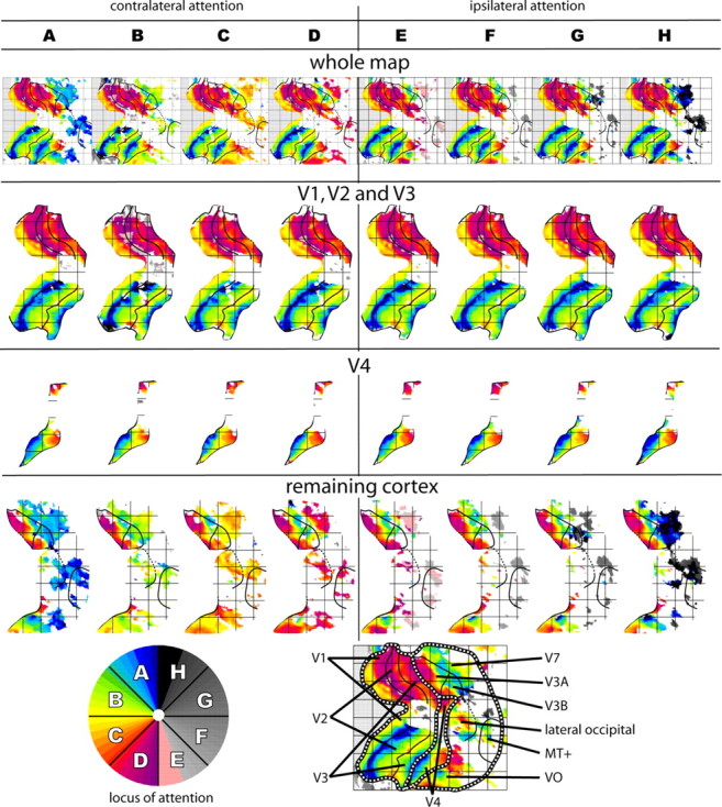
Modulation of spatial tuning by attention: map examples. Columns A–H show angular mapping data acquired during attention to a single contralateral wedge. The scale at the bottom left indicates the attended wedge for each panel. Top row, Each map represents one-eighth of the data acquired from subject 1 right hemisphere. The more that attention shifts the spatial tuning estimates, the more the colors change across columns. To aid visualization, the maps in the top row have been divided into three parts: V1/V2/V3 (second row), where attentional modulations are negligible and the colors barely change; V4 (third row), where attentional modulations are moderate and the colors change slightly; the remainder of cortex on the map (bottom row), including regions where attentional modulations are dramatic and the colors change vividly.

Figure 8.

Modulation of spatial tuning by attention: ROI analysis. ROIs were defined in all hemispheres in which both foveal/parafoveal data (for dorsal V4 ROI assignment) and attentional data (for attention analysis) were available. The ROIs themselves were defined by the foveal/parafoveal data, and the data analyzed within the ROIs are the attentional data. The top row shows upper-field ROIs; the bottom row shows lower-field ROIs. Modulation of spatial tuning by attention is quantified as S_match. This index increases as spatial tuning shifts toward the attended wedge, and it is not artificially inflated by noise. An unmodulated ROI would have an S_match of 1; larger values represent greater modulation toward attended wedges (upper limit 8). Error bars give the SE, calculated for each ROI by jackknifing. S_match in upper-field ventral V4, lower-field ventral V4, and lower-field dorsal V4 are not significantly different from one another but are significantly different from S_match in both upper- and lower-field portions of the neighboring regions V3 and lateral occipital (lat-occ). LH, Left hemisphere; RH, right hemisphere.

Degrees of modulation within the various ROIs were quantified using an index, S_match (see Materials and Methods). This index allowed us to compare degrees of modulation within and across V4 and other areas. Upper- and lower-field ROIs were created using spatial tuning from maps obtained by averaging across all attention conditions (supplemental Figs. 4–6, available at www.jneurosci.org as supplemental material), except when the coarse 3 × 3 × 3 mm voxel size did not permit boundary transitions to be distinguished. In the latter case, ROIs were created using the spatial tuning from the foveal/parafoveal maps. An ROI not modulated by attention has S_match = 1, and an ROI where spatial tuning shifts toward the attended wedge has S_match > 1. Because there are eight wedges, S_match can reach a maximum of 8.

Figure 8 gives S_match for all hemispheres and ROIs. S_match in lateral occipital is significantly higher (p < 0.05; all p values by two-tailed t test across hemispheres) than S_match in both dorsal and ventral V4. This result supports our conclusion from the topography that V4 and lateral occipital are distinct. S_match in dorsal V4 is significantly higher (p < 0.01) than S_match in V3d. This result supports our conclusion from the topography that dorsal V4 and V3d are distinct.

S_match in dorsal V4 is not significantly different (p > 0.8) from S_match in ventral V4 lower field and also is not significantly different (p > 0.3) from S_match in ventral V4 upper field. In addition, S_match in ventral V4 lower and upper field are not significantly different from each other (p > 0.15). These results support our conclusion from the topography that dorsal V4, ventral V4 lower field, and ventral V4 upper field are all portions of a single visual area, V4.

In lateral occipital, S_match is quite high (Fig. 8), reflecting the degree to which attention modulates estimates of spatial tuning in this area. Note that it is not correct to infer an absence of topography based on observed attentional modulation of estimated spatial tuning (see Discussion). However, observing large attentional modulations does imply that spatial tuning estimates in that part of the brain are at least partially dependent on the specific tasks and stimuli used during individual mapping experiments.

Discussion

These experiments indicate that human cortex anterior to V3d plus V3v consists of a dorsal and a ventral region that together comprise a single second-order transformation of contralateral visual space.

Comparisons with macaque

We call these human regions dorsal V4 and ventral V4 because they share multiple defining properties with macaque V4d and V4v (Fig. 9). First, both species exhibit dorsal and ventral topographic organization anterior to V3d plus V3v. Second, in both species the dorsal and ventral topographic regions meet in the fovea. Third, in both species the V4 topography is laid out similarly: The upper field and a limited portion of the lower field are represented ventrally, anterior/lateral to ventral V3 (Gattass et al., 1988), and the parafoveal lower field is represented dorsally, anterior/lateral to parafoveal V3d.

Figure 9.

Macaque V4 and human V4. Data are formatted as in Figure 1. To aid in comparison, the top row is repeated from the bottom row of Figure 1 (macaque V4); the plots represent neurophysiological responses to stimuli located at ≤30°. The bottom two rows depict the organization observed in two individual human subjects; these plots represent fMRI spatial tuning estimates to stimuli located at ≤5°. The figure as a whole illustrates that macaque V4 and human V4 share remarkably similar topographic organizations.

Macaque area V4 (Felleman and Van Essen, 1991; Gattass et al., 1988) is also called the V4 complex to acknowledge redundant visual field coverage within its borders (Van Essen and Zeki, 1978) and has been subdivided into V4-proper and V4A (Zeki, 1983) and into DLc and DLr (Stepniewska et al., 2005). [Note that V4t is equivalent to part of MTc (Stepniewska et al., 2005), not to V4A/DLr.] However, the relevant macaque topography has not been measured in detail [for coarse maps, see Gattass et al. (1988) and Fize et al. (2003); for detailed but cropped maps, see Brewer et al. (2002)]. If future macaque maps support a V4-proper (DLc) plus V4A (DLr) distinction, it may be interesting to investigate analogies between macaque V4-proper plus V4A (DLc plus DLr) and human V4 plus lateral occipital.

The human V4 data differ from accepted macaque V4 properties in two respects. First, in macaque V4v, spatial tuning substantially below the horizontal meridian has been seen only at eccentricities of approximately ≥20°, with only a hint at lower eccentricities [Gattass et al. (1988), their Fig. 9]. In human ventral V4, spatial tuning substantially below the horizontal meridian is seen at much lower eccentricities (Fig. 6). If this apparent difference is not an artifact of sparse sampling in macaque, the off-horizontal V4 discontinuity occurs, on average, at somewhat lower angles in humans (Fig. 9).

Second, farthest-peripheral tuning in our V4 data are restricted to the upper field, so peripheral visual field coverage is asymmetric. The same observation appears on other groups' maps (e.g., Wade et al., 2002). In macaque V4, several studies (Gattass et al., 1988; Boussaoud et al., 1990; Felleman and Van Essen, 1991; Fize et al., 2003) depicted an upper-field-biased surface area asymmetry, but because the lower field extends to at least 30° (Gattass et al., 1988; Stepniewska et al., 2005), the visual field coverage asymmetry is mild. It is unclear why peripheral visual field coverage in human V4 maps is so asymmetric. Possible explanations include asymmetries in distance to other visual areas [hence, the cost of developing and maintaining topographic connections is asymmetric; compare concepts by Mitchison (1991) and Van Essen (1997)], asymmetries in neuronal receptive field size (hence, symmetric stimuli evoke responses of asymmetric magnitude), or some fMRI artifact(s) consistently obscuring the V4 lower periphery only. Alternatively, although we observed no topographic transition dividing the upper periphery from the rest of V4, the upper periphery might belong to a different area [compare a previous argument for relieving surface area asymmetry by reassigning part of macaque V4 upper periphery (Stepniewska et al., 2005) and VMO below (Tyler et al., 2005)].

Previous schemes that conflict conceptually with our V4

Regions hV4 plus LO1, defined by Wade et al. (2002) and Larsson and Heeger (2006), respectively, are conceptually interrelated. The hV4 plus LO1 parcellation defines cortex anterior to human V3d plus V3v as two first-order transformations, hV4 (ventral) and LO1 (dorsal). This organization would be unique to humans among studied primates. Our results, however, indicate that human cortex anterior to V3d plus V3v consists of a single second-order transformation, as in New World (Pinon et al., 1998) and Old World (Gattass et al., 1988; Stepniewska et al., 2005) monkeys.

The map transitions bounding ventral V4 (Fig. 3) replicate most of the hV4 boundaries (Wade et al., 2002; Brewer et al., 2005). However, ventral V4 differs from hV4 in three ways. First, hV4 does not include the part of upper-field ventral V4 extending into the cortical fovea and meeting dorsal cortex, so transition R (Fig. 3) is unique to our study. Second, hV4 has no dorsal complement. Third, although hV4 is called a hemifield, spatial tuning estimates there typically lack the lower-field parafovea [Larsson and Heeger (2006), their Fig. 7]; our dorsal V4 fills in the gap. For clarity, we note a remaining difference. The hV4 map does not separate peripheral V3v from the VO maps [Brewer et al. (2005), their Figs. 4, 5], but in some of our hemispheres (Fig. 11), the V4 upper periphery separates peripheral V3v from the VO maps. Note that local variability at the merger of the V3v, ventral V4, and VO map peripheries would impact neither our main conclusions nor those of the hV4 authors. Larger stimuli will be needed to characterize this region more conclusively.

Figure 11.

Our V4 parcellation in a chronological context. The locations of various regions described in the literature are shown. Because the ventral map literature has been particularly controversial, the figure focuses on a ventral view. The figure does not include the converging lines of evidence that support our scheme over hV4+LO1 and V4v/V4d-topo+V8; for this material, see Figure 10 and the Discussion. The panels show a single map segmented according to boundaries used in several studies that focused on different aspects of the data. We attempt to portray each set of boundaries objectively, but the figures in the original studies may better reflect the authors' intended claims. The map itself is from our parafoveal/peripheral across-attention dataset (subject 1 LH), which provides good coverage of the peripheral region where several boundary schemes overlap. The central small white disk in the angle color legend is a reminder that the central ±1° was unstimulated in the parafoveal/peripheral angle experiments (see Materials and Methods). The eccentricity color legend is scaled to account for the center-of-mass bias inherent in the analysis of the eccentricity m-sequence data (see Materials and Methods) and uses different colors to avoid confusion with the foveal/parafoveal maps in previous figures. U, Upper visual field; L, lower visual vield; UL, both upper and lower visual field; CaS, calcarine sulcus; POS, parieto-occipital sulcus; CoS, collateral sulcus; FuG, fusiform gyrus. A, Field-sign-defined V4v (no dorsal component defined). B, Meridian-defined V4v (no dorsal component defined). C, V4v, as in B, and V8. D, hV4 (no dorsal component defined), VO-1, and VO-2. E, V4 (equivalent to hV4; no dorsal component defined), VMO, and VOF. F, Ventral V4 (paired with dorsal V4). Ventral V4 overlaps with field-sign-defined V4v, with meridian-defined V4v plus additional cortex, with a small part of V8, with hV4 plus additional cortex (as shown here, plus the extension of the upper field into the foveal confluence visible in the foveal/parafoveal data from Fig. 4), and with part of VMO. Ventral V4 does not overlap with the majority of V8, with VO-1, or VO-2 (given some variability at farthest-peripheral upper-field ventral V4), or with VOF.

The anterior boundary of dorsal V4 falls in the middle of LO1 as defined by Larsson and Heeger (2006). The difference between dorsal V4 and LO1 boundaries is shown as an overlay on our subject 2 RH (Fig. 10A). We chose this hemisphere because its topography strongly resembles that in the first LO1 exemplar [Larsson and Heeger (2006), their Fig. 1, top panels] and so establishes that data from both laboratories are comparable. Although putative hV4/LO1/LO2 boundaries can be delineated, the mapping data (in this hemisphere and the Larsson and Heeger exemplar) leave a lower-field parafoveal gap in hV4. The gap can be seen on visual coverage plots of hV4 [Larsson and Heeger (2006), their Fig. 7], or on maps by identifying cortex tuned to lower-field angles and comparing eccentricity tuning in the identical location. The hV4 gap begs the question of whether part of LO1 might be the missing part of hV4.

Figure 10.

Our V4 parcellation versus alternative parcellations (hV4+LO1 and V4v/V4d-topo+V8). A, Right-hemisphere maps from our subject 2. This hemisphere is very similar to that in the first exemplar hemisphere from the LO1 study [the right hemisphere of subject 8 in Fig. 1 of Larsson and Heeger (2006) (LH 2006)]. In both, an elongated patch of upper-field angles appears within lateral occipital, roughly parallel to the anterior boundary of parafoveal V3d. This patch is the defining feature of the putative LO1 anterior boundary (dark blue arrow, as in the dark blue top vertical meridian; compare our anterior dorsal V4 boundary, marked with a yellow arrow as in the yellow horizontal meridian). B, Right-hemisphere maps from our subject 1. As in A, the ventral V4 data do not include parafoveal-stimulated eccentricities at lower-field angles. However, in this hemisphere, the lateral occipital topographic patterns do not include the defining feature of the LO1/LO2 boundary, described above. Instead, multiple reversing upper- and lower-field stripes run roughly at right angles to the isoangle contours in dorsal V4 and to the parafoveal V3d boundary. C, The relationship between our V4 and V4v/V4d-topo+V8 is illustrated as a schematic adapted from that in Tootell and Hadjikhani (2001) (TH 2001). The V4v/V4d-topo scheme predicted that in the future, a V4d parallel would be found within V4d-topo (lavender); our dorsal V4 (yellow overlay) fulfills that prediction. D, A series of tests demonstrates that our V4 scheme (HKG) accounts better for the available data than hV4+LO1 or V4v/V4d-topo+V8. ①, Point 1 was central to Tootell and Hadjikhani (2001). ②, The hV4+LO1 scheme requires hV4 to be a complete hemifield. Problematically, the LO1/LO2 scheme describes hV4 as a hemifield, but the hV4 visual field coverage plots (Larsson and Heeger, 2006) are closer to quadrant V3v. ③, Uniquely human features in visual cortex are rare enough to be perceived as exceptional (Preuss 2004), so claims of human uniqueness require compelling data (see Discussion).

Figure 10B shows a different hemisphere (our subject 1 RH) where the data are consistent with V4, but not with LO1. Larsson and Heeger (2006) do acknowledge substantial variability in LO1 and LO2. However, the LO1 plus LO2 argument posits that LO1/LO2 variability is attributable to some type(s) of error, based on an explicit assumption that topographic maps in LO1 and LO2 should be as consistent across hemispheres as maps in V1, V2, and V3 (Larsson and Heeger, 2006). We contend that this assumption is without basis in the literature and that the large, variable topographic gaps and irregularities compromise the claim that LO1 and LO2 are visual areas (because the basis for presenting them as visual areas is the premise that the data consistently cover continuous hemifields).

The LO1/LO2 boundary criterion is field-sign reversal. To support this criterion, Larsson and Heeger (2006) call reversals the “gold standard for defining visual area boundaries retinotopically.” This description is straightforward but is unsupported by citation or the literature as a whole. For example, neighboring capuchin areas PO and POd are not separated by a reversal, but each area covers the visual hemifield (Neuenschwander et al., 1994). Similarly, neighboring macaque regions V4-proper and V4A (DLc/DLr) share the same field sign but have redundant visual field coverage (Van Essen and Zeki, 1978), and the question of whether they are parts of a single area is debated (Stepniewska et al., 2005). Conversely, it is conceivable that local reversals, large enough to appear in BOLD maps, might occur inside coarsely topographic visual areas [compare smaller local reversals within V2 (Roe and Ts'o, 1995; Shipp and Zeki, 2002)].

Other previous schemes

Field-sign-defined V4v (Sereno et al., 1995), meridian-defined V4v (DeYoe et al., 1996), V4d-topo (Tootell and Hadjikhani, 2001), V8 (Hadjikhani and Tootell, 1998), V3B defined by Smith et al. (1998), DLO (Tyler et al., 2005), VMO (Tyler et al., 2005) and lateral occipital (Hagler et al., 2006) overlap in part with V4. In general, comparisons with these regions (Figs. 10, 11; Table 2) involve precise boundary locations rather than conceptual issues and are discussed in the supplemental material (available at www.jneurosci.org).

Attentional effects on estimated spatial tuning

Our attentional data show that fMRI spatial tuning in some extrastriate regions depends on attention, consistent with claims that some extrastriate regions code visual responses nonretinally (Connor et al., 1996; Grill-Spector et al., 1999). The mechanism could reflect BOLD amplitude changes (Kastner et al., 1998; Tootell et al., 1998; Brefczynski and DeYoe, 1999; Smith et al., 2000; Silver et al., 2005), or neuronal receptive field shifts (Connor et al., 1996).

Spatial tuning modulations do not imply absence of topography. For example, attention modulates lateral occipital spatial tuning, but neighboring cortical locations still respond best to neighboring visual locations (local progression of topographic contours) (Fig. 4), and specific cortical locations respond to only some attended wedges (S_match is high but under 8). Large modulations simply imply nonretinal input, such that point-to-point organization might be described more accurately as topographic than as retinotopic.

References

- Allman JM, Kaas JH. The organization of the second visual area (VII) in the owl monkey: a second order transformation of the visual hemifield. Brain Res. 1974;76:247–265. doi: 10.1016/0006-8993(74)90458-2. [DOI] [PubMed] [Google Scholar]
- Boussaoud D, Ungerleider LG, Desimone R. Pathways for motion analysis: cortical connections of the medial superior temporal and fundus of the superior temporal visual areas in the macaque. J Comp Neurol. 1990;296:462–495. doi: 10.1002/cne.902960311. [DOI] [PubMed] [Google Scholar]
- Brainard DH. The psychophysics toolbox. Spat Vis. 1997;10:433–436. [PubMed] [Google Scholar]
- Brefczynski JA, DeYoe EA. A physiological correlate of the “spotlight” of visual attention. Nat Neurosci. 1999;2:370–374. doi: 10.1038/7280. [DOI] [PubMed] [Google Scholar]
- Brewer AA, Press WA, Logothetis NK, Wandell BA. Visual areas in macaque cortex measured using functional magnetic resonance imaging. J Neurosci. 2002;22:10416–10436. doi: 10.1523/JNEUROSCI.22-23-10416.2002. [DOI] [PMC free article] [PubMed] [Google Scholar]
- Brewer AA, Liu J, Wade AR, Wandell BA. Visual field maps and stimulus selectivity in human ventral occipital cortex. Nat Neurosci. 2005;8:1102–1109. doi: 10.1038/nn1507. [DOI] [PubMed] [Google Scholar]
- Connor CE, Gallant JL, Preddie DC, Van Essen DC. Responses in area V4 depend on the spatial relationship between stimulus and attention. J Neurophysiol. 1996;75:1306–1308. doi: 10.1152/jn.1996.75.3.1306. [DOI] [PubMed] [Google Scholar]
- Crick F, Jones E. Backwardness of human neuroanatomy. Nature. 1993;361:109–110. doi: 10.1038/361109a0. [DOI] [PubMed] [Google Scholar]
- Desimone R, Schein SJ. Visual properties of neurons in area V4 of the macaque: sensitivity to stimulus form. J Neurophysiol. 1987;57:835–868. doi: 10.1152/jn.1987.57.3.835. [DOI] [PubMed] [Google Scholar]
- DeYoe EA, Carman GJ, Bandettini P, Glickman S, Wieser J, Cox R, Miller D, Neitz J. Mapping striate and extrastriate visual areas in human cerebral cortex. Proc Natl Acad Sci USA. 1996;93:2382–2386. doi: 10.1073/pnas.93.6.2382. [DOI] [PMC free article] [PubMed] [Google Scholar]
- Dougherty RF, Koch VM, Brewer AA, Fischer B, Modersitzki J, Wandell BA. Visual field representations and locations of visual areas V1/2/3 in human visual cortex. J Vision. 2003;3:586–598. doi: 10.1167/3.10.1. [DOI] [PubMed] [Google Scholar]
- Efron B, Tibshirani R. An introduction to the bootstrap. New York: Chapman and Hall; 1993. [Google Scholar]
- Felleman DJ, Van Essen DC. Distributed hierarchical processing in the primate cerebral cortex. Cereb Cortex. 1991;1:1–47. doi: 10.1093/cercor/1.1.1-a. [DOI] [PubMed] [Google Scholar]
- Fize D, Vanduffel W, Nelissen K, Denys K, Chef d'Hotel C, Faugeras O, Orban GA. The retinotopic organization of primate dorsal V4 and surrounding areas: a functional magnetic resonance imaging study in awake monkeys. J Neurosci. 2003;23:7395–7406. doi: 10.1523/JNEUROSCI.23-19-07395.2003. [DOI] [PMC free article] [PubMed] [Google Scholar]
- Gallant JL, Braun J, Van Essen DC. Selectivity for polar, hyperbolic, and Cartesian gratings in macaque visual cortex. Science. 1993;259:100–103. doi: 10.1126/science.8418487. [DOI] [PubMed] [Google Scholar]
- Gallant JL, Connor CE, Rakshit S, Lewis JW, Van Essen DC. Neural responses to polar, hyperbolic, and Cartesian gratings in area V4 of the macaque monkey. J Neurophysiol. 1996;76:2718–2739. doi: 10.1152/jn.1996.76.4.2718. [DOI] [PubMed] [Google Scholar]
- Gattass R, Sousa AP, Gross CG. Visuotopic organization and extent of V3 and V4 of the macaque. J Neurosci. 1988;8:1831–1845. doi: 10.1523/JNEUROSCI.08-06-01831.1988. [DOI] [PMC free article] [PubMed] [Google Scholar]
- Grill-Spector K, Kushnir T, Edelman S, Avidan G, Itzchak Y, Malach R. Differential processing of objects under various viewing conditions in the human lateral occipital complex. Neuron. 1999;24:187–203. doi: 10.1016/s0896-6273(00)80832-6. [DOI] [PubMed] [Google Scholar]
- Hadjikhani N, Liu AK, Dale AM, Cavanagh P, Tootell RB. Retinotopy and color sensitivity in human visual cortical area V8. Nat Neurosci. 1998;1:235–241. doi: 10.1038/681. [DOI] [PubMed] [Google Scholar]
- Hagler DJ, Jr, Sereno MI. Spatial maps in frontal and prefrontal cortex. NeuroImage. 2006;29:567–577. doi: 10.1016/j.neuroimage.2005.08.058. [DOI] [PubMed] [Google Scholar]
- Hansen KA, David SV, Gallant JL. Parametric reverse correlation reveals spatial linearity of retinotopic human V1 BOLD response. NeuroImage. 2004a;23:233–241. doi: 10.1016/j.neuroimage.2004.05.012. [DOI] [PubMed] [Google Scholar]
- Hansen KA, Kay KN, Gallant JL. Spatial attention biases BOLD retinotopic maps of intermediate visual areas. Soc Neurosci Abstr. 2004b;34:717–4. [Google Scholar]
- Huk AC, Dougherty RF, Heeger DJ. Retinotopy and functional subdivision of human areas MT and MST. J Neurosci. 2002;22:7195–7205. doi: 10.1523/JNEUROSCI.22-16-07195.2002. [DOI] [PMC free article] [PubMed] [Google Scholar]
- Kaas JH. Topographic maps are fundamental to sensory processing. Brain Res Bull. 1997;44:107–112. doi: 10.1016/s0361-9230(97)00094-4. [DOI] [PubMed] [Google Scholar]
- Kaas JH. Early visual areas: V1, V2, V3, DM, DL, and MT. In: Kaas JH, editor. The primate visual system. Boca Raton, FL: CRC; 2004. pp. 139–160. [Google Scholar]
- Kastner S, De Weerd P, Desimone R, Ungerleider LG. Mechanisms of directed attention in the human extrastriate cortex as revealed by functional MRI. Science. 1998;282:108–111. doi: 10.1126/science.282.5386.108. [DOI] [PubMed] [Google Scholar]
- Kay KN, Hansen KA, David SV, Gallant JL. Artifacts in phase-encoded fMRI retinotopic mapping. Soc Neurosci Abstr. 2005;35:508–12. [Google Scholar]
- Kobatake E, Tanaka K. Neuronal selectivities to complex object features in the ventral visual pathway of the macaque cerebral cortex. J Neurophysiol. 1994;71:856–867. doi: 10.1152/jn.1994.71.3.856. [DOI] [PubMed] [Google Scholar]
- Larsson J, Heeger DJ. Two retinotopic visual areas in human lateral occipital cortex. J Neurosci. 2006;26:13128–13142. doi: 10.1523/JNEUROSCI.1657-06.2006. [DOI] [PMC free article] [PubMed] [Google Scholar]
- McKeefry DJ, Zeki S. The position and topography of the human colour centre as revealed by functional magnetic resonance imaging. Brain. 1997;120:2229–2242. doi: 10.1093/brain/120.12.2229. [DOI] [PubMed] [Google Scholar]
- Mitchison G. Neuronal branching patterns and the economy of cortical wiring. Proc Biol Sci. 1991;245:151–158. doi: 10.1098/rspb.1991.0102. [DOI] [PubMed] [Google Scholar]
- Neuenschwander S, Gattass R, Sousa APB, Pinon MC. Identification and visuotopic organization of areas PO and POd in Cebus monkey. J Comp Neurol. 1994;340:65–86. doi: 10.1002/cne.903400106. [DOI] [PubMed] [Google Scholar]
- Pasupathy A, Connor CE. Responses to contour features in macaque area V4. J Neurophysiol. 1999;82:2490–2502. doi: 10.1152/jn.1999.82.5.2490. [DOI] [PubMed] [Google Scholar]
- Pelli DG. The VideoToolbox software for visual psychophysics: transforming numbers into movies. Spat Vis. 1997;10:437–442. [PubMed] [Google Scholar]
- Pinon MC, Gattass R, Sousa AP. Area V4 in Cebus monkey: extent and visuotopic organization. Cereb Cortex. 1998;8:685–701. doi: 10.1093/cercor/8.8.685. [DOI] [PubMed] [Google Scholar]
- Press WA, Brewer AA, Dougherty RF, Wade AR, Wandell BA. Visual areas and spatial summation in human visual cortex. Vision Res. 2001;41:1321–1332. doi: 10.1016/s0042-6989(01)00074-8. [DOI] [PubMed] [Google Scholar]
- Preuss TM. Specializations of the human visual system: the monkey model meets human reality. In: Kaas JH, Collins CE, editors. The primate visual system. Boca Raton, FL: CRC; 2004. pp. 231–260. [Google Scholar]
- Reynolds JH, Chelazzi L. Attentional modulation of visual processing. Annu Rev Neurosci. 2004;27:611–647. doi: 10.1146/annurev.neuro.26.041002.131039. [DOI] [PubMed] [Google Scholar]
- Roe AW, Ts'o DY. Visual topography in primate V2: multiple representations across functional stripes. J Neurosci. 1995;15:3689–3715. doi: 10.1523/JNEUROSCI.15-05-03689.1995. [DOI] [PMC free article] [PubMed] [Google Scholar]
- Sereno MI, Tootell RB. From monkeys to humans: what do we now know about brain homologies? Curr Opin Neurobiol. 2005;15:135–144. doi: 10.1016/j.conb.2005.03.014. [DOI] [PubMed] [Google Scholar]
- Sereno MI, Dale AM, Reppas JB, Kwong KK, Belliveau JW, Brady TJ, Rosen BR, Tootell RB. Boundaries of multiple visual areas in humans revealed by functional magnetic resonance imaging. Science. 1995;268:889–893. doi: 10.1126/science.7754376. [DOI] [PubMed] [Google Scholar]
- Shipp S, Zeki S. The functional organization of area V2, II: the impact of stripes on visual topography. Vis Neurosci. 2002;19:211–231. doi: 10.1017/s0952523802191176. [DOI] [PubMed] [Google Scholar]
- Silver MA, Ress D, Heeger DJ. Topographic maps of visual spatial attention in human parietal cortex. J Neurophysiol. 2005;94:1358–1371. doi: 10.1152/jn.01316.2004. [DOI] [PMC free article] [PubMed] [Google Scholar]
- Smith AT, Greenlee MW, Singh KD, Kraemer FM, Hennig J. The processing of first- and second-order motion in human visual cortex assessed by functional magnetic resonance imaging (fMRI) J Neurosci. 1998;18:3816–3830. doi: 10.1523/JNEUROSCI.18-10-03816.1998. [DOI] [PMC free article] [PubMed] [Google Scholar]
- Smith AT, Singh KD, Greenlee MW. Attentional suppression of activity in the human visual cortex. NeuroReport. 2000;11:271–277. doi: 10.1097/00001756-200002070-00010. [DOI] [PubMed] [Google Scholar]
- Stepniewska I, Collins CE, Kaas JH. Reappraisal of DL/V4 boundaries based on connectivity patterns of dorsolateral visual cortex in macaques. Cereb Cortex. 2005;15:809–822. doi: 10.1093/cercor/bhh182. [DOI] [PubMed] [Google Scholar]
- Swisher JD, Halko MA, Merabet LB, McMains SA, Somers DC. Visual topography of human intraparietal sulcus. J Neurosci. 2007;27:5326–5337. doi: 10.1523/JNEUROSCI.0991-07.2007. [DOI] [PMC free article] [PubMed] [Google Scholar]
- Tootell RB, Hadjikhani N. Where is “dorsal V4” in human visual cortex? Retinotopic, topographic and functional evidence. Cereb Cortex. 2001;11:298–311. doi: 10.1093/cercor/11.4.298. [DOI] [PubMed] [Google Scholar]
- Tootell RB, Reppas JB, Dale AM, Look RB, Sereno MI, Malach R, Brady TJ, Rosen BR. Visual motion aftereffect in human cortical area MT revealed by functional magnetic resonance imaging. Nature. 1995;375:139–141. doi: 10.1038/375139a0. [DOI] [PubMed] [Google Scholar]
- Tootell RB, Mendola JD, Hadjikhani NK, Ledden PJ, Liu AK, Reppas JB, Sereno MI, Dale AM. Functional analysis of V3A and related areas in human visual cortex. J Neurosci. 1997;17:7060–7078. doi: 10.1523/JNEUROSCI.17-18-07060.1997. [DOI] [PMC free article] [PubMed] [Google Scholar]
- Tootell RB, Hadjikhani N, Hall EK, Marrett S, Vanduffel W, Vaughan JT, Dale AM. The retinotopy of visual spatial attention. Neuron. 1998;21:1409–1422. doi: 10.1016/s0896-6273(00)80659-5. [DOI] [PubMed] [Google Scholar]
- Tyler CW, Likova LT, Chen CC, Kintsevich LL, Schira MM, Wade AR. Extended concepts of occipital retinotopy. Curr Med Imaging Rev. 2005;1:319–329. [Google Scholar]
- Ungerleider LG, Mishkin M. Two cortical visual systems. In: Ingle DJ, Mansfield RJW, Goodale MS, editors. The analysis of visual behavior. Cambridge, MA: MIT; 1982. pp. 549–586. [Google Scholar]
- Van Essen DC. A tension-based theory of morphogenesis and compact wiring in the central nervous system. Nature. 1997;385:313–318. doi: 10.1038/385313a0. [DOI] [PubMed] [Google Scholar]
- Van Essen DC. Organization of visual areas in macaque and human cortex. In: Chalupa LM, Werner JS, editors. The visual neurosciences. Cambridge, MA: MIT; 2004. [Google Scholar]
- Van Essen DC, Gallant JL. Neural mechanisms of form and motion processing in the primate visual system. Neuron. 1994;13:1–10. doi: 10.1016/0896-6273(94)90455-3. [DOI] [PubMed] [Google Scholar]
- Van Essen DC, Zeki SM. The topographic organization of rhesus monkey prestriate cortex. J Physiol (Lond) 1978;277:193–226. doi: 10.1113/jphysiol.1978.sp012269. [DOI] [PMC free article] [PubMed] [Google Scholar]
- Van Essen DC, Lewis JW, Drury HA, Hadjikhani N, Tootell RB, Bakircioglu M, Miller MI. Mapping visual cortex in monkeys and humans using surface-based atlases. Vision Res. 2001;41:1359–1378. doi: 10.1016/s0042-6989(01)00045-1. [DOI] [PubMed] [Google Scholar]
- Wade AR, Brewer AA, Rieger JW, Wandell BA. Functional measurements of human ventral occipital cortex: retinotopy and colour. Philos Trans R Soc Lond B Biol Sci. 2002;357:963–973. doi: 10.1098/rstb.2002.1108. [DOI] [PMC free article] [PubMed] [Google Scholar]
- Wandell BA, Brewer AA, Dougherty RF. Visual field map clusters in human cortex. Philos Trans R Soc Lond B Biol Sci. 2005;360:693–707. doi: 10.1098/rstb.2005.1628. [DOI] [PMC free article] [PubMed] [Google Scholar]
- Zeki S. The distribution of wavelength and orientation selective cells in different areas of monkey visual cortex. Proc R Soc Lond B. 1983;217:449–470. doi: 10.1098/rspb.1983.0020. [DOI] [PubMed] [Google Scholar]