A Simple Connectivity Scheme for Sparse Coding in an Olfactory System

Abstract

Recent studies, using unbiased sampling of neuronal activity in vivo, indicate the existence of sparse codes in the brain. These codes are characterized by highly specific, associative (i.e., dependent on combinations of features) and often invariant neuronal responses. Sparse representations present many advantages for memory storage and are, thus, of wide interest in sensory physiology. Here, we study the statistics of connectivity in an olfactory network that contributes to the generation of such codes: Kenyon cells (KCs), the intrinsic neurons of the mushroom body (a structure involved in learning and memory in insects) receive inputs from a small population of broadly tuned principal neurons; from these inputs, KCs generate exquisitely selective responses and, thus, sparse representations. We find, surprisingly, that KCs are on average each connected to about 50% of their input population. Simple analysis indicates that such connectivity indeed maximizes the difference between input vectors to KCs and helps to explain their high specificity.

Introduction

Ever since the study by Ramon y Cajal (1990), neuroscientists have recognized that network connectivity must play a key role in brain function. On a large scale, connectivity is clearly not random (Sporns and Tononi, 2002; Song et al., 2005): interneuronal connections thus result from some optimization process. The constraints acting on this optimization are physical (e.g., to minimize wiring length), developmental (address specification has limits defined by genetics and developmental rules), and functional; for example, networks should be stable, but also able to switch states rapidly (Tsodyks and Sejnowski, 1995) and particular dynamics (e.g., synchronization) require particular types of connectivity (Traub et al., 1999). Finally, connectivity must be constrained also by computation; associativity, for instance, requires convergence and arbitrariness (Fuster, 2000). How these different pressures eventually shaped and optimized neural circuits is a fascinating problem. Marr (1969) and Albus (1971) were among the very first to address this issue. In his explorations of cerebellar architecture, Marr (1969) examined the statistics of connectivity between mossy fibers, granule, Golgi, and Purkinje cells in the context of memory functions (e.g., pattern association, capacity). His work may be the first to point to localized versus distributed strategies for pattern storage.

Studies in mammals (including humans), in songbirds, and in insects (Thompson and Best, 1989; Rolls and Tovee, 1995; Vinje and Gallant, 2000; Hahnloser et al., 2002; Laurent, 2002; Perez-Orive et al., 2002, 2004; DeWeese et al., 2003; Olshausen and Field, 2004; Quian Quiroga et al., 2005) reveal that activity in some neural populations is very sparse, specific (Willmore and Tolhurst, 2001), and in some instances, invariant to low-level features (Stopfer et al., 2003). The firing of such neurons usually occurs on a low background of baseline activity; thus, each action potential carries a lot of information. In these coding schemes, each stimulus evokes responses in only a small subset of neurons. Conversely, each neuron responds to only a small subset of stimuli; such neurons are often called “grandmother” or “cardinal neurons.” Early work by Attneave (1954), Barlow (1969), and Marr (1969), as well as more recent theoretical work (Willshaw and Longuet-Higgins, 1970; Kanerva, 1988; Tsodyks and Feigel'man, 1988; Perez-Vicente and Amit, 1989; Garcia-Sanchez and Huerta, 2003; Huerta et al., 2004; Olshausen and Field, 2004) noted the potential relevance of such coding schemes: they can increase the capacity of associative networks and be beneficial for learning, classification, and read-out in noisy systems. The experiments we report here examine the issue of network connectivity and its relationship to representation sparseness, using a small, well defined, and easily accessible system, the locust olfactory system. We ask the following question: what are the statistics of connectivity between a small population of nonspecific principal neurons [the projection neurons (PNs) of the antennal lobe] and their targets [the Kenyon cells (KCs) of the mushroom body], whose responses are highly specific? We then examine the surprising (yet, in hindsight, straightforward) combinatorial implications of these results for representation sparseness.

Materials and Methods

Physiology

Preparation and odor stimulation.

Results were obtained from young adult locusts (Schistocerca americana) of either sex taken from an established, crowded colony. Locusts were immobilized, with both antennae intact for olfactory stimulation. The brain was exposed, desheathed, and superfused with locust saline, as described previously (Laurent and Naraghi, 1994). Odors were delivered by injection of a controlled volume of odorized air within a stream of desiccated, carbon-filtered air, custom-designed to maintain a constant flow over time. Odor pulses of 1 s duration were delivered at a minimum interval of 10 s. Teflon tubing was used at and downstream from the mixing point to prevent odor lingering and cross-contamination. Odors were used at 100% vapor pressure, further diluted in the desiccated air stream. Odorants used were pentanol, hexanol, hexanal, cis-3-hexen-1-ol, heptanol, isoamyl acetate (Aldrich, Milwaukee, WI), cineole, geraniol (Sigma, St. Louis, MO), cherry (Bell Flavor and Fragrances, Northbrook, IL), and clean air. Odors were delivered for the sole purpose of cell identification: all measurements geared toward estimating PN–KC connectivity were done using spikes produced during spontaneous activity.

Intracellular and LFP recordings.

Intracellular and local field potential (LFP) recording was done using an Axoclamp-2B amplifier (Molecular Devices, Union City, CA). KCs were impaled in their soma with intracellular borosilicate micropipettes (DC resistance, ∼250–400 MΩ) pulled on a Sutter horizontal puller and filled with 0.5 m potassium acetate. Intracellular recordings of PNs were done with similar micropipettes with a DC resistance of ∼150–300 MΩ. Local field potentials were recorded in the mushroom body calyx, using saline-filled heat-polished patch pipettes (DC resistance, ∼5–10 MΩ). LFPs were amplified online with gain 1000× using a Brownlee (San Jose, CA) 440 amplifier. KC firing threshold (voltage) was that measured at the time of peak d²V_m/dt² preceding spike peak, minus mean membrane potential (V_m) before odor-pulse onset (see Fig. 6A, bottom right).

Figure 6.

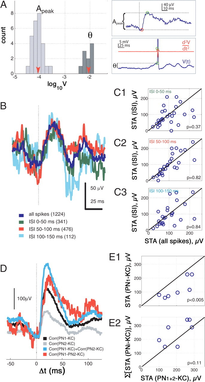
KC firing threshold and summation. A, Histograms of PN–KC EPSP peak-amplitudes (A_peak) and KC threshold values (θ) plotted on the same logarithmic scale (log₁₀V). PN–KC EPSPs are very small and mostly distributed around 60–110 μV. KC thresholds are mostly within 5–10 mV. Means of distributions are indicated by arrowheads. Note that two orders of magnitude of voltage separate the two distributions. Insets, Top, A_peak is the difference between peak voltage and voltage before EPSP onset. Bottom, KC firing threshold θ, calculated for odor-evoked spikes, defined as the membrane potential at the time of peak of the second time derivative of the membrane potential before the spike peak, minus the mean membrane potential before odor-pulse onset. B, C, No evidence is found for paired-pulse facilitation (or depression). B, Examples of spike-triggered averages calculated from one PN–KC pair using only spikes with preceding ISIs in ranges indicated. All ISI-STAs are aligned on the voltage at the time of EPSP onset in the STA including all the spikes. Note that ISI-STAs are more noisy than the STA for all spikes, because events available for averaging are much fewer (up to 10-fold). C1–C3, Group data over all connected pairs showing that peak amplitude distributions for ISIs as in B (indicated in top left of scatter plots) are not significantly different from controls (all spikes). D, E, EPSP summation is near-linear when close to V_rest. D, STAs of two PN–KC pairs [corr(PN1-KC), black; corr(PN2-KC), gray; same KC for PNs 1 and 2], compared with STA constructed using only spikes from the two PNs occurring within 0–15 ms of each other [corr(PN1-PN2-KC), red]. Arithmetic sum of black and gray STAs is shown in blue. Slightly sublinear summation occurs in this example. E1, E2, Group data over pairs fulfilling conditions as in D and analyzed in the same way. E1, Combined-event STAs (abscissa) were always larger than any single-event STAs with the same PNs (ordinate; p < 0.005), indicating summation. E2, Most combined-event STAs (abscissa) were slightly smaller (6 of 7 experiments), although not statistically different from the arithmetic sum of single-event STAs for the same PN (ordinate), indicating that EPSP summation is close to linear within this range of V_m.

Tetrode recordings.

Extracellular recordings were done with silicon probes generously provided by the University of Michigan Center for Neural Communication Technology. Tetrodes were placed within soma clusters in the antennal lobe, and the tissue was allowed to stabilize around the probe tips for 30 min. Custom-built 16-channel preamplifiers (×1) and amplifiers (×10,000) were used. Data from each channel were acquired continuously (15 kHz/channel, 12 bit), filtered online (custom-built amplifiers, bandpass 0.3–6 kHz), and stored on computer memory.

Data acquisition and analysis.

Electrophysiological data (intracellular, extracellular and LFP) were acquired using a NI-DAQ acquisition board (National Instruments, Austin, TX) via the LabView (National Instruments) interface. Data analysis was performed using Matlab (Mathworks, Natick, MA) and Igor (WaveMetrics, Lake Oswego, OR).

Spike sorting.

Tetrode recordings were analyzed as described previously (Pouzat et al., 2002). Briefly, events were detected on all channels as voltage peaks above a preset threshold (usually 2.5–3.5 times each channel's SD). For any detected event on any channel, the same 3 ms window (each containing 45 samples) centered on that peak was extracted from each one of the four channels in a tetrode. Each event was then represented as a 180-dimension vector (4 × 45 samples). Noise properties for the recording were estimated from all the recording segments between detected events by computing the auto- and cross-correlations of all four channels. A noise covariance matrix was computed and used for noise whitening. Events were then clustered using a modification of the expectation maximization algorithm. Because of noise whitening, clusters consisting of, and only of, all of the spikes from a single source should form a Gaussian (SD, 1) distribution in 180-dimension space. This property enabled us to perform several statistical tests to select only units that met quantifiable criteria of cluster isolation. Categories 1 and 2 required that each cluster contain no event classified as belonging to a different cluster, within a 7- and 5-SD envelope, respectively, around its cluster center (supplemental information part 1 and supplemental Fig. 1, available at www.jneurosci.org as supplemental material). Category 3 required at least 5 SDs between cluster centers. Connectivity analysis was done using only clusters that (1) passed all standard tests [interspike interval (ISI) distribution, SD, and projection tests] (Pouzat et al., 2002) and (2) belonged to above categories 1 and 2. Spike sorting, tests, and assignment of separation quality were done before assessing connectivity.

Spike-triggered statistics and connectivity assessment.

KC membrane potential was correlated with PN firing over a time window of ±300 ms from the PN spike detection time to produce a spike-triggered average (STA) (Moore et al., 1970; Jack et al., 1971; Mendell and Henneman, 1971; Cope et al., 1987; Kang et al., 1988; Komatsu et al., 1988; Laurent and Burrows, 1989; Mason et al., 1991; Matsumura et al., 1996). The delay was measured from the detection-threshold crossing by the extracellular PN spike (∼200 μs before peak) to the onset of the EPSP, determined as the peak of the second time derivative of voltage. STAs were calculated with PN spike clusters of categories 1 and 2 above, only if at least 200 spikes of spontaneous PN activity were available and if KC membrane potential was stable over the time of recording. The existence of a connection between a PN and KC was assessed using three methods. For methods 1 and 2, the STAs were bandpass filtered (Butterworth sixth order digital filter, band 2–1000 Hz), smoothed by convolution with a Gaussian (SD, 1 ms); 5% were trimmed off their start/end margins to cancel edge effects resulting from this preprocessing. Method 1 was based on the correlation between time of peak voltage (t_max[V], generally corresponding to EPSP peak in the STA) and time of peak time-derivative (t_max[dV/dt], generally corresponding to the middle of EPSP rising phase). We defined the section (0 < t_max[dV/dt] < t_max[V] < +40ms) of the t_max[V], t_max[dV/dt] space (see Fig. 2C,D) as corresponding to EPSPs. All PN–KC pairs yielding (t_max[V], t_max[dV/dt]) pairs within this section were thus counted as connected. Method 2 defined as EPSPs those STAs for which V(t) crossed v = 2.5 SD of the average STA voltage within the time interval [0, +50ms], and crossed v_1/2 = 1.25 SD only once within the time interval [0, (t | V(t)= v)]. Method 3 relied on visual inspection of the STAs: time delay and waveform were the critical features (see Fig. 2B, asterisks). To address particular issues such as facilitation or EPSP summation, STAs were computed with special constraints; we thus also allowed cases with <200 spikes. ISI-STAs were computed by selecting as triggers only spikes separated from the previous one by a delay that fell within a defined range. Combined events between two PNs were defined as events where spikes from both PNs fell within ≤15 ms of each other (average time-to-peak); the trigger for averaging was the first action potential of the two.

Figure 2.

Synaptic connections between PNs and KCs occur with ∼0.5 probability. A, Superimposed intracellular voltage traces from one KC (black) triggered from spontaneous extracellular spikes of one PN (PN spike at Δt = 0). V_KC (red), Average of 1,000 sweeps, revealing an EPSP-shaped waveform with a delay of ∼5 ms from the PN spike (see Results for PN–KC convergence). B, STAs from 14 different PN–KC pairs (STA in A is fifth from top). STAs were selected only on the basis of unit isolation (highest quality category) (see Materials and Methods) and sorted according to the numbers of traces used for the average (indicated for each average). Vertical calibration, 100 μV. Asterisks indicate pairs classified by eye as synaptic connections. Note (conduction plus synaptic) delay δ. C–D2, Method 1 for classifying STAs into connected versus unconnected. C, The peak times of the averaged intracellular voltage (t_max[V_m]; red dot) and of its time derivative (t_max[dV_m/dt]; green dot) are indicated for each of six PN–KC pairs. The numbers of spikes used for each STA are indicated in brackets. Left column, Three examples classified as connected (with high, intermediate, and low spike numbers); right column, three examples classified as not connected, with comparable spike numbers. Note that t_max[V_m], t_max[dV_m/dt], and Δt = 0 are clustered (left) and scattered (right). Vertical calibration, 100 μV. D1, D2, Scatter plot of all the data that passed quality criteria (categories 1 and 2) (see Materials and Methods). t_max[V_m] is plotted against t_max[dV_m/dt]; points within window ([0,40ms]) suggest direct connection, with added condition that t_max[dV_m/dt] < t_max[V_m]. The expanded section in D2 shows a tight cluster of STAs, indicative of connection. E, Statistics of connectivity, as determined with three different classification tests (methods 1–3) (see Materials and Methods). PN–KC pairs are treated independently. All three tests find the mean probability of connection between a PN and a KC to be around 0.5. F, Distribution of connectivity measured between individual KCs and the PNs recorded simultaneously with those KCs. KCs connected to ∼50% of simultaneously recorded PNs form the largest group.

Simulated EPSPs.

To assess the effect of PN firing statistics on STA shape, EPSPs were modeled using the α-function, A(t) = α te^−αt (Rall, 1967; Jack and Redman, 1971), with α = 0.075 ms⁻¹, which fits the rise and decay of “clean” STA-EPSPs (i.e., ones calculated from PNs whose spontaneous discharge deviated the least from Poisson statistics). Postsynaptic V_m was modeled by linearly summing the α-functions, a constant delay (5 ms, based on the PN–KC STAs) after each PN spike time, taken either from our recordings or from an artificial distribution with chosen statistics. We added Gaussian noise (SD equal to the α-function peak amplitude) to the modeled KC potential with some tests. Quantification of similarity between these modeled STAs and the real KC STAs was done using three separate measures: correlation coefficient, root-mean-square (RMS) error, and “fit,” (as defined here, fit computes how well two vectors match in their rising and falling phases). The rise-fall vector s(x), where x is a vector of continuous values, is defined as s(x) = sign(dx/dt), and the fit is the scalar product of two rise-fall vectors, normalized by their size, producing +1 for identity, −1 for “flipped” waveforms, and 0 for randomly correlated ones.

Anatomy

KCs and PNs from adult locusts (Schistocerca americana) were filled using intracellular electrodes containing 1 m LiCl and tip-filled with either 10% Lucifer yellow (PNs and KCs) or 10 mm Alexa Fluor 568 (Invitrogen, Eugene, OR) (KCs). Five-hundred-millisecond-long pulses of negative current (2–7 nA) were applied at 1 Hz for 5 min (KCs) or 30 min (PNs). After 10–30 min diffusion time, brains were fixed in situ with 5% formaldehyde in deionized water for 30 min. Brains were dissected out, washed in water for 2 h, dehydrated in ethanol, cleared, mounted in methyl-salycilate, and imaged on a Zeiss (Oberkochen, Germany) confocal microscope system. For each cell, stacks of images were taken through the brain and exported for analysis. The profiles of the neurons were isolated from the background using a dedicated Matlab (Mathworks) script. The calyx was manually outlined for each reconstruction using Scion (Frederick, MD) Image. Isolated neurons and their traced calyces were exported to Imaris (Bitplane AG Scientific Solutions, St. Paul, MN) where three-dimensional volumes were rendered using the Surpass function. Rendered images were exported as .tif files and prepared for publication using Photoshop (Adobe, San Jose, CA).

Results

Hints of high PN convergence onto Kenyon cells

Using an in vivo preparation (for details about the locust olfactory system and odor-evoked activity, see supplemental information part 2, available at www.jneurosci.org as supplemental material), we recorded KC activity intracellularly, mushroom body LFP extracellularly, and antennal lobe PN spike output using tetrodes (see Materials and Methods) (Fig. 1A,B). Because PN axon collaterals branch throughout the mushroom body calyx, LFPs are nearly identical across the entire calyx (Laurent and Naraghi, 1994) and reflect both mean activity and coherence of the PN population's spiking output. Confirming previous observations (Perez-Orive et al., 2002, 2004; Stopfer et al., 2003), most KCs had extremely low background firing rates (mean, 0.052 spike/s; median, 0.001 spikes/s) and always responded to odors with subthreshold oscillations of membrane potential, locked to the LFP (Fig. 1B). These membrane potential oscillations are caused by phase-delayed nicotinic excitation (from PNs) and GABA-ergic inhibition (from lateral horn interneurons) (Perez-Orive et al., 2002). Careful inspection of such recordings revealed that the instantaneous variations of KC membrane potential were often highly correlated with those of the LFP, both during odors (Fig. 1B,C) and during baseline (Fig. 1B,D). For each one of 42 KCs tested with the odor pentanol, we calculated the cross-correlation between membrane potential and LFP; we then identified, for each trial (n = 512), the time lag at which the correlation was the highest. The values of peak correlation and corresponding time lag are plotted against each other in Figure 1E (red triangles). Correlation coefficients were distributed around 0.3 and tracked the LFP with very little jitter (±5 ms). The same analysis was performed with 22 PNs recorded intracellularly from their soma in the antennal lobe. In this case, peak correlations were smaller, and distributed broadly in time (Fig. 1E, squares). If, as initially assumed (Perez-Orive et al., 2002), individual KCs are contacted by only few PNs, how could their membrane potential reflect so well the activity of the PN population as reported by LFPs? This suggested that individual KCs might receive inputs from a larger fraction of the PN population than we initially estimated. We next looked for direct physiological evidence for synaptic connections between the two cell populations.

Figure 1.

Intracellular voltage in single KCs is correlated with local field potentials. A, Reconstruction of the dendritic tree of a KC within the mushroom body calyx (top) and of two PNs (red and green) filled simultaneously within the same antennal lobe (bottom). PN somata and axons lie above and below the plane of glomerular projections. PNs and KC were stained by intracellular injection of Lucifer yellow. B, Simultaneous recording of mushroom body LFP (top, red), KC intracellular voltage (middle, black) and six single-unit PNs (bottom, raster plots) in response to an odor (cis-3-hexen-1-ol, horizontal bar indicates odor delivery; top) and at baseline (bottom). Note V_m oscillations in response to odor and correlation between Vm and LFP. Calibrations: vertical, 10 mV (V_m), 1 mV (LFP); horizontal, 1 s. C–E, KC membrane potential is highly correlated with the LFP. C, D, Examples of filtered KC V_m (KC_f) and LFP recorded simultaneously, and sliding cross-correlograms averaged over nine such trials (bottom). Note frequent covariations of amplitude between KC and LFP in both odor (C; pentanol, black bar) and baseline (D) conditions. KC_f and LFP filtered with the same 5–50 Hz bandpass digital filter. The look-up table represents correlation coefficients: (C) −0.4 (blue) to +0.4 (red); (D) −0.07 (blue) to +0.07 (red). Calibrations: vertical, 1mV (KCf), 100μV (LFP); horizontal, 1 s. E, Plot of peak correlation coefficients between LFP and V_m traces (5 ms time bins) versus time delay for which correlation coefficient is maximal (Δt_max), for 42 KCs (red triangles) and 22 PNs (blue squares). Each Δt_max is the median over 7–20 trials (pentanol, 512 trials total). KCs and PNs lock to the LFP at different phases; the relevant parameter is the variance of Δt_max, indicating tightness of coupling between single-cell membrane voltage and LFP.

PN–KC convergence: direct electrophysiological measurements

Spiking activity was recorded extracellularly from PNs in the antennal lobe using silicon-based tetrode arrays (Fig. 1B). In locusts, PNs are the only antennal lobe neurons that produce sodium action potentials (Laurent and Davidowitz, 1994): all spikes so detected could thus be unambiguously attributed to PNs. In each recording session, spikes from 2–10 well isolated PN clusters (Pouzat et al., 2002) (for criteria, see Materials and Methods, supplemental Fig. 1, available at www.jneurosci.org as supplemental material) were taken. We simultaneously recorded intracellularly from the soma (6–8 μm diameter) (Leitch and Laurent, 1996) of one randomly chosen KC anywhere in the ipsilateral mushroom body (Fig. 1A,B). These KCs responded to all odors tested with subthreshold oscillations, indicating that they received olfactory input; among 42 KCs, only three showed a reliable spiking response to one of the tested odors, consistent with previous results (Perez-Orive et al., 2002). Because PNs tend to synchronize transiently with one another during responses to odors (Laurent and Davidowitz, 1994; Wehr and Laurent, 1996; Mazor and Laurent, 2005), we used PN spikes produced solely during spontaneous activity (Fig. 1B, bottom, baseline) to signal-average KC intracellular voltage traces (see Materials and Methods). PN spikes during baseline (2.5–4 spikes/s) are not correlated across PNs over short time scales (see below). For a number of PN–KC pairs, STAs of KC voltage revealed, after much averaging, an EPSP-shaped waveform, with a clearly defined delay (δ) of 5.81 ± 0.9 ms (mean ± SD, n = 28) (Fig. 2A,B). Separate experiments (Perez-Orive et al., 2004) measured the PN spike conduction delay between the antennal lobe and the mushroom body calyx at 4.6 ± 0.7 ms (n = 6 PNs). The remaining ∼1 ms is consistent with known delays at insect central cholinergic synapses (Laurent and Burrows, 1989). PNs are known from electron-microscopy to make direct chemical synapses onto KCs (Distler and Boeckh, 1997). We thus interpret these STAs as representing EPSPs generated directly by the recorded PN onto the recorded KC.

EPSP amplitudes were very small and narrowly distributed (86 ± 44 μV, n = 28) (see below). Because EPSPs were always much smaller than the SD of the intracellular voltage trace (Fig. 2A), they were revealed only after averaging many hundreds of sweeps (Fig. 2B). Over all recordings, we selected 57 PN–KC pairs for which recording conditions matched our selection criteria (low intracellular recording noise, stability, stationarity and separability of PN clusters) (see Materials and Methods), and used them to estimate the connection probability between the two cell populations. We obtained a variety of STAs (Fig. 2B, 14 examples are shown); in a subset (Fig. 2B, asterisks), we detected the shape and delays consistent with direct synaptic connections. We used three methods to assess whether each STA should be classified as indicative of a direct connection (Fig. 2C,D) (see Materials and Methods). With all three methods, ∼50% of the STAs were classified as indicating direct PN–KC connections (Fig. 2E). Assuming that our classification of STAs is correct and that our sampling is random, this sample size indicates that the PN–KC connection probability (over the entire population) lies between 0.36 and 0.63 (p < 0.05), and that individual KCs each receive ∼400 PN inputs. Because we often sampled several PNs simultaneously with each Kenyon cell intracellular recording, we could also assess the connection probabilities over these subsets. The most commonly sampled KCs were those that appeared to be connected with half of the PNs that had been recorded simultaneously (Fig. 2F).

Effects of PN firing statistics

The shape and delay of the STAs were generally consistent with those of monosynaptic EPSPs. Yet, some STAs had complicated shapes (e.g., membrane potential sag around EPSP proper) (Fig. 2A,B), warranting additional analysis. We show here that those nonclassical shapes are spurious effects of PN firing statistics. Consider for instance a hypothetical neuron that fires action potentials at regular 100 ms intervals. The STA of the membrane potential in a postsynaptic neuron would reveal not only a shape consistent with an EPSP right after the presynaptic spike, but also other similarly shaped events at ±100 ms intervals around it. In a more realistic case, in which presynaptic firing contains an oscillatory component around 10 Hz, the spike-triggered average would, in addition to the EPSP waveform, contain deflections of decreasing amplitude at intervals of about ±100 ms around trigger time. Other features linked to presynaptic spike discharge, such as refractoriness, could have yet additional consequences on the shape of the STA (e.g., a sag before EPSP onset time). Even though our averages were all calculated from long sequences of PN activity at baseline, thus ruling out strong 20 Hz periodicity, interspike-interval statistics might have introduced biases. We thus examined the contribution of PN baseline discharge statistics on the shape of the averaged EPSPs. We used the spike trains of each recorded PN to average the voltage of a putative monosynaptic target, in which the EPSP was modeled as an α-function (Rall, 1967; Jack and Redman, 1971) (Fig. 3A) (see Materials and Methods). The shape modulation of the averaged model waveform was then compared with that of the recorded KC (Fig. 3B), using three different metrics (fit, correlation, and RMS error) (see Materials and Methods). With all three metrics, the model waveform predicted the shape of the real STA better than the α-function alone (p < 0.0001, 0.005, and 0.0001, respectively) (Fig. 3B,C). We conclude that PN baseline-discharge statistics account for our observations on averaged EPSPs.

Figure 3.

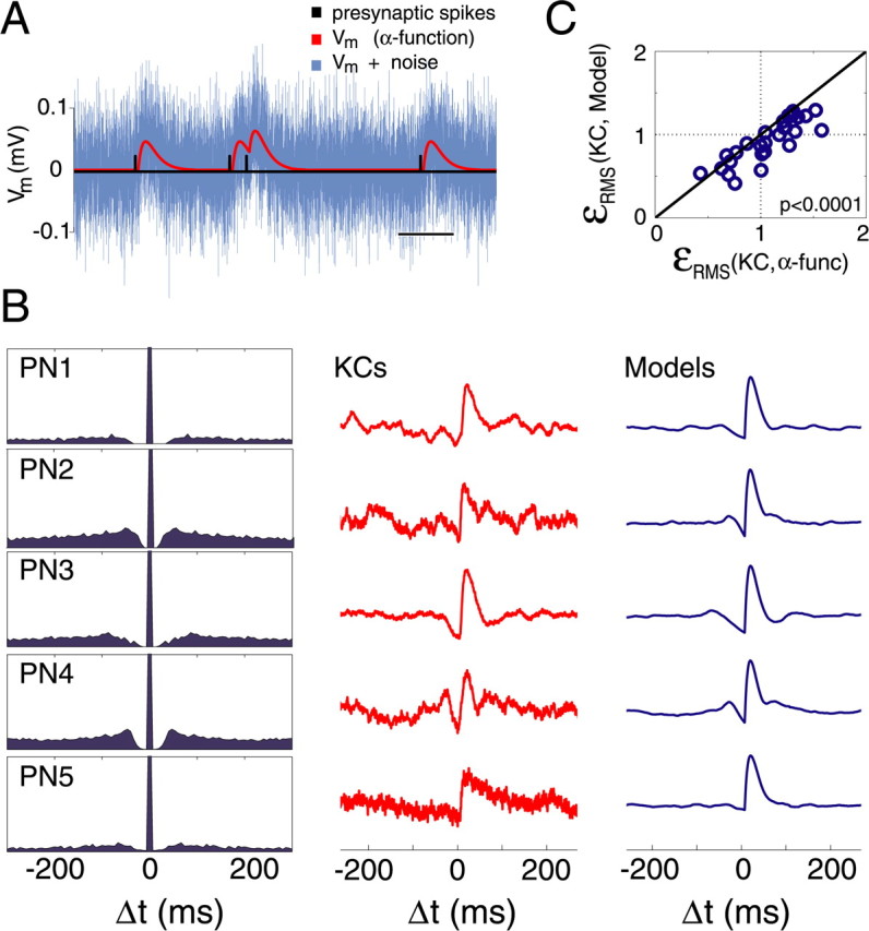
STA waveform around the EPSP is explained by non-Poisson firing statistics of PNs at rest. A, Model KC membrane potential data are generated by triggering an α function 5 ms after each spike of a recorded PN. Black, Segment of recorded PN-spike time series; red, model V_m; cyan, model V_m plus Gaussian noise (for details, see Materials and Methods). Horizontal calibration, 100 ms. The vertical scale is arbitrary. B, Examples of STAs calculated for (connected) PN–KC pairs (KCs) compared with those computed by applying the model EPSPs to the same PN spikes trains (Models). Left, Autocorrelation function for each PN spike train (PNi). Note that potential deflections around EPSPs (KCs) are well explained by PN firing statistics. C, RMS error between KC STAs and model STAs is smaller than between KC STAs and the α-function (p < 0.0001).

We next considered the possibility that high PN–KC connectivity was an artifact of high inter-PN correlations. We reasoned that, if the path between a recorded PN and a recorded KC is indirect, jitter caused by the interposed PNs would produce detectable changes in the STAs. As a test, we introduced into the PN spike times artificial jitter drawn from uniform distributions bounded at ±1, 2, 5, 10 and 20 ms (Fig. 4A) and calculated the new STAs. Jitter between 5 and 10 ms blunted the rising phase of the STAs: their onset occurred at or before the spike time of the presumed presynaptic PN (Fig. 4A). With 20 ms jitter, the STAs began before the trigger and lost the asymmetric shape characteristic of EPSPs (fast rise, slow decay) (Fig. 4A), ruling out the possibility that we would classify them as connections. Overall, we observed that the risk of misclassification would be significant only if PN–PN cross-correlations were high within the interval [−10, +10 ms]. We then calculated PN–PN cross-correlations with 75 pairs of PN spike-trains recorded simultaneously (with separate tetrodes, to eliminate the possibility of misclassifying superposed spike events; 5–20 min of baseline spiking); all were inconsistent with this hypothesis (Fig. 4B–D). Cross-correlations were generally flat around Δt = 0; the distributions of cross-correlation values just around 0 (e.g., [−5, +5 ms]) were not significantly different from those for wider intervals (Fig. 4C,D) or from those calculated for randomly shuffled trials (i.e., correlations did not exceed chance levels given their firing rates). Finally, we note that electrical synapses or dye coupling have, thus far, never been found between PNs or between KCs in adult locusts. We conclude that the averaged KC EPSPs are unlikely to be artifacts of high inter-PN correlations, and must therefore reflect direct PN–KC connections.

Figure 4.

Inter-PN spike correlations do not affect estimates of PN–KC connectivity. A, Effect of introducing jitter in PN spike times (to simulate PN–PN correlations) on the computed KC membrane potential STA. Jitter is drawn from uniform distributions (0 to 0–20 ms). Note the gradual effect of jitter on EPSP shape and particularly the elimination of spike-to-EPSP delay for jitters with max ≥5ms. False classification (method 3) of a PN–KC STA as a connection would thus require PN–PN spike-time correlations at rest to be high at −10 ms <Δt <10 ms and low around this interval. B1, B2, Cross-correlation between spike trains of two simultaneously recorded PNs computed over 1 ms bins (red). Gray lines are cross-correlations calculated over shuffled trials. Insets, Sample rasters (right) and corresponding auto-correlations (left). B1, Cross-correlation over ±300 ms lags. The box at 0 is expanded in B2. B2, Cross-correlation over lag of ±35 ms. Black bar, Interval [−5,+5] ms; pink bars, intervals [−10, −6], and [+6,+10] (used to compute distributions in C and D). Note that no peak in correlation can be seen within a tight interval and that correlation levels (red) are similar to chance level expected from the ISI distribution alone (shuffled trials, gray). C, Frequency histogram of the peak correlation coefficients above chance within intervals [−5,+5] ms (black) and [−10, −6], [+6,+10] ms (pink) for 75 PN pairs analyzed as in B. Overlap of black and pink is shown in brown. Peak correlation values are small (<0.005) and those for the central interval are not statistically different from those calculated for the larger interval (p = 0.42). D, Frequency histogram of summed correlation coefficients above chance (summed over all bins within corresponding intervals) for the same 75 PN pairs as in C. The summed coefficient over an interval corresponds to the probability of observing a spike from one PN within that interval from a spike of another. Summed correlation values are small and distributed around 0 (within ±0.01), and those for the central interval are not statistically different from those for the larger one (p = 0.75). B–D, Data from PN pairs recorded simultaneously from separate tetrodes, to avoid erroneous elimination of events containing spike superpositions, over 5–20 min of spontaneous activity.

Anatomical overlap between PN axons and KC dendrites

We next examined the extent of spatial overlap between PN axon collaterals and KC dendrites in the mushroom body, by labeling both cell types either as individuals or in groups of two or three neurons. One hundred KCs and 65 PNs were individually labeled with Alexa Fluor or Lucifer yellow; the calyx arbors of 15 PN axons and 79 KCs were reconstructed fully, in three dimensions, from confocal stacks (see Materials and Methods), and for 30 of these KCs, together with the entire surrounding calyx. Figure 5A shows the dendritic trees of two KCs stained in one mushroom body (top), and the axonal terminals of three PNs stained in the mushroom body of a different animal (bottom). Typical of all intracellular fills examined, PN axons give off two to four dorsal axonal collaterals as they run ventral to the calyx (Fig. 5A, front view); these collaterals branch so extensively within the calyx that the axonal terminals of only those three (among 830) PNs delineate and fill the entire calyx (Fig. 5A, top view). In contrast with published observations in fruit flies (Marin et al., 2002; Wong et al., 2002), we observed no zonal or heterogeneous innervation of the calyx by individual PN axon collaterals. Consistent with observations in other insects (Strausfeld et al., 1998), including Drosophila, KCs had, in contrast, restricted dendritic trees confined to a small volume of the calyx (Fig. 5A) and were distributed homogeneously within the calyx. The linear dendritic span of individual KCs extended, depending on the KC, over 1/8 to 1/2 of the unfolded calyx (along all three spatial axes). Because of the extensive PN axonal projections, the dendrites of individual KCs always overlapped with the axon of any one PN examined. In fifteen concurrent fills of one PN axon and one KC (Fig. 5B,C), we could identify between one and four sites of PN–KC axodendritic juxtaposition within <1 μm. Although we do not know when these appositions represent true synaptic contacts, we note that there appears to be no morphological restriction on PN–KC connectivity. Detailed examination of the dendritic trees of 12 KCs (eight filled with Alexa Fluor, four filled with cobalt hexamine and intensified with silver) revealed that each neuron contained on average 135 terminal branches (range, 87–205), each likely to receive several synaptic contacts. Because in locusts PN axon collaterals terminate only in the main (outer) calyx (Farivar, 2005), most KC terminal branches likely contact PN axons. This suggests that individual KCs are contacted by numbers of PNs commensurate with our electrophysiological estimates (half of 830 PNs).

Figure 5.

Extensive overlap between PN axon collaterals and KC dendrites in the mushroom body. A, Reconstructions of the calyx of the mushroom body (yellow, from background autofluorescence). The top row shows two KC dendritic trees (cyan and purple) from three different views. KCs were filled within the same calyx with Lucifer yellow as described in the text. The bottom row shows the axonal arbor of three PNs (red) from the same three views, filled simultaneously with Lucifer yellow, in a different animal. B, Reconstruction showing one KC (green) and axon collaterals of one PN (red) filled in the same brain. The KC was filled with Alexa Fluor 568; the PN was filled with Lucifer yellow. C, Magnified (ray-traced) reconstruction of processes of KC and PN in B. Asterisks indicate sites where KC dendrites and PN axons are ≤1 μm apart, as measured in the original three-dimensional stack.

Estimating Kenyon cell firing threshold

Whereas KCs reliably respond to odors with subthreshold oscillations (Fig. 1B), they respond with an action potential only extremely rarely (Perez-Orive et al., 2002, 2004; Stopfer et al., 2003; Laurent and Naraghi, 1994). Previous analyses of PN responses to odors (Mazor and Laurent, 2005) indicate that each oscillation cycle contains between 100 and 150 PN spikes; of those spikes, 55% originate from a small number of PNs that fire reliably in that cycle (10%, or ∼80 of all 830 PNs) and 45% from less reliable PNs (∼30% or ∼250 of all PNs). All other PNs (60% of total) are reliably inhibited. At each oscillation cycle, the identities of the active (reliable and unreliable) and inactive PNs change in an odor-specific manner (Wehr and Laurent, 1996; Mazor and Laurent, 2005). We attempted here to estimate the number of coincident PN inputs required to bring the membrane potential of a KC beyond spiking threshold. Figure 6A shows the measured amplitudes of PN-evoked EPSPs in KCs (A_peak) and of KC spike thresholds (θ) as distributions on a logarithmic scale. The averaged peak EPSP amplitude was A_peak = 86 ± 44 μV, with over half of all EPSPs between 60 and 110 μV (Fig. 6A). The mean KC spike threshold (Table 1, θ), measured over all trials in which a spiking response had been produced during the odor pulse, was θ = 8.9 ± 3.5 mV (n = 10) (Fig. 6A). Assuming perfect spike synchrony among PNs and linear summation by KCs (see Discussion), we deduce that ∼100 concurrent PN inputs (of ∼400 anatomical PN inputs on average per KC) are needed to trigger an action potential in a KC. This estimate also relies on the assumption that we can use the EPSPs' mean amplitude for our calculations, even if their distribution is not Gaussian; this assumption is justified by the central limit theorem (see supplemental information part 3, available at http//www.jneurosci.org as supplemental material). We will call f this firing threshold (in numbers of simultaneous PN inputs) (Table 1).

Table 1.

List of abbreviations and symbols used in this paper

n	Number of PNs in the antennal lobe [830 (Leitch and Laurent, 1996)]
a	Number of PNs active during an oscillation cycle [100–150 (Mazor and Laurent, 2005)]
m	Number of PNs sampled by one average KC (present study)
K	Number of possible combinations of m among n PNs (equals the number of possible PN input patterns to KCs)
k	Number of KCs in one mushroom body [50,000 (Leitch and Laurent, 1996)]
f	KC firing threshold, in numbers of simultaneous PNs (present study)
θ	KC firing threshold, in millivolts (present study)

See also Discussion and supplemental material (available at www.jneurosci.org).

Short-term plasticity at the PN–KC synapse

The existence of short-term depression or facilitation at this synapse would force us to refine our estimates of f in several ways. First, it could lead to major increases or decreases of our estimate. Second, it could suggest that our measurements of true unitary EPSPs are underestimated by our averaging procedure, because of high failure rates. Because low release probability is generally correlated with facilitation (Katz and Miledi, 1968; Dobrunz and Stevens, 1997), we first looked for evidence of homosynaptic plasticity. We calculated the spike-triggered averages for the PN–KC pairs classified as connected, using only spikes that were separated from the preceding one by a particular interval (ISIs 0–50, 50–100, and 100–150 ms, respectively) (Fig. 6B). STAs produced by these selected spikes were, on average, no different from those produced using all spikes (Fig. 6C1–C3) (p = 0.37, 0.82, 0.84, respectively). This result is inconsistent with significant homosynaptic facilitation and, thus, with high failure rates at the PN–KC synapse. This reinforces our confidence in the estimate of unitary EPSP amplitudes.

We next looked for evidence of heterosynaptic effects on the summation of PN-evoked EPSPs in KCs. For this we selected experiments in which (1) at least two PNs had been recorded simultaneously with one KC, (2) where those PNs had both been identified as being connected to the KC, and (3) where the PN spikes originated from different tetrodes (thus avoiding waveform clustering problems that arise in cases of superposition). Seven PN–KC triplets fulfilled these requirements. We selected those PN spikes (from each one of the simultaneously recorded sets) that occurred within <15 ms of one another (corresponding to the time to EPSP peak recorded at the KC soma) and used the first one of each pair to calculate the spike-triggered average of the KC membrane potential (Fig. 6D, red trace). We then compared this compound EPSP to the arithmetic sum of each average calculated separately (Fig. 6D, blue trace). In all cases (Fig. 6E1), the compound EPSP was larger than each unitary EPSP alone (p = 0.0045). In all but one case, the compound EPSP was equal to or smaller than the arithmetic sum of the mean unitary EPSPs measured at their peaks (Fig. 6E2) (p = 0.11). (That the compound EPSP amplitude was often less than the sum of the EPSP peaks is explained by the fact that, in most cases, one EPSP was in its rising phase while the other was at its peak.) These results indicate that, although EPSPs from separate sources do summate, they do so without facilitation and without supralinear enhancement, at membrane potentials close to rest.

Discussion

In locust, each KC appears to be contacted on average by about half of the PN population (415 ± 54 of n = 830 PNs) by weak synapses. Extrapolating from physiology alone, the firing threshold of KCs (f, in numbers of PN spikes) would lie close to 1/4 of that number (∼100), a number commensurate with the mean total number of PN spikes produced per each oscillation cycles during an odor response (100–150) (Mazor and Laurent, 2005) but, as discussed below, probably unrealistically high. Note that the total PN spike output varies little over 1000-fold variations in odor concentration (Stopfer et al., 2003) or with odor complexity (K. Shen and G. Laurent, unpublished observations). Technical issues are discussed in the supplemental information (parts 2, 3), available at http//www.jneurosci.org as supplemental material. We examine here the functional significance of these findings.

A connectivity that maximizes differences between input vectors

The dense connectivity between PNs and KCs was puzzling, because it seemed incompatible with the high response selectivity of KCs (Perez-Orive et al., 2002). Simple combinatorics, however, suggest otherwise: if each KC samples m PNs out of n (Table 1), and if those connections are distributed randomly, the number K of possible PN combinations that KCs could sample is given by the binomial coefficient, K(m) = m!/n!(n-m)!, where K is maximum for m = n/2 and decreases symmetrically around that value. For n = 800 PNs and m ≈ n/2 = 400, K ≈ 10²⁴⁰, an enormous number. Because there are only k = 50,000 KCs in each locust mushroom body, only as many connection patterns can be realized out of all K; assuming (based on anatomy) that PN-KC connections are distributed approximately randomly, these connection patterns should be very different from one another on average (the probability that two KCs might sample the same PNs is 10⁻²⁴⁰ ≈ 0). In fact, the difference between input vectors obeys a binomial distribution such that most pairs of input vectors differ from each other by ∼200 PNs (half of the mean number of inputs to each). These principles, previously explored with theoretical networks of binary units (Kanerva, 1988), might be a key to the design of some associative networks. If thresholds are chosen appropriately (see below), individual KCs will respond to very few and different stimuli, thus producing sparse coding by sets of specific neurons. At the same time, the high convergence of PNs onto individual KCs explains why the membrane potential of each KC is noticeably correlated with the LFP (Fig. 1B–E), an observation that seemed paradoxical. In conclusion, connectivity with half probability can maximize the differences between input vectors to KCs and, thus, increase their response selectivity. Note that nonrandom structure in the PN–KC connection matrix (as might exist because of individual experience or evolutionary biases) could modify our conclusions. But given the enormous numbers of combinations suggested by our experimental measurements, only very strong connection biases would likely change our conclusions qualitatively.

Firing thresholds and sparseness

Although 50% connectivity maximizes differences between input vectors, it does not, on its own, explain why target-cell responses are rare: sparsening must rely also on an appropriate adjustment of global strength of the input and synaptic integration/spike threshold in the target neurons. As noted previously, part of the solution lies in the observations (1) that the number of active PNs per oscillation cycle (Table 1, a) is limited to ∼100–150 (Mazor and Laurent, 2005), (2) that PNs rarely fire more than once per oscillation cycle and (3) that temporal integration of PN input by KCs is limited to single half-oscillations-cycles (Perez-Orive et al., 2002; 2004). These results define an upper bound for the firing threshold of KCs (which we called f), compatible with our experimental estimates (f ≈ 100): if f were higher than a, no KC would ever fire. In fact, even if KC firing thresholds were slightly smaller than a, the probability that one KC would fire would still be infinitesimally small, because there exist only k = 50,000 KCs of all the possible K = 10²⁴⁰ input vectors to KCs; that is, the probability that all, or nearly all, a active PNs converge on the same KC among all k is infinitesimally small. Our intuition is therefore that f should be significantly less than a so as to ensure that some KCs at least can be activated by any PN pattern. We now explore quantitatively the relationships between KC firing threshold (f, in numbers of PN inputs) and KC response probabilities, given what our experiments revealed about PN activity (a) and PN–KC connectivity (m ≈ n/2).

Of n PNs in the antennal lobe, we previously measured the number (a) that are active (rarely producing more than one spike) during an average oscillation cycle (Mazor and Laurent, 2005). An average KC samples m PNs. Of the K possible combinations of m PNs among n, only k = 50,000 are realized in a mushroom body. We knew n and k (Leitch and Laurent, 1996); we now have experimental estimates for m [≈ n/2 (present study)] and a [100–150 (Mazor & Laurent, 2005)]. We will now estimate the average KC firing threshold f (in numbers of coincident PN action potentials) such that a given fraction of the k KCs can be activated reliably during an oscillation cycle; we thus wish to determine the relationship between f and KC response probability p(f) in an average KC. That probability can be expressed as follows (for derivation, see supplemental information part 4, available at www.jneurosci.org as supplemental material):

We plot p(f) for n = 800 PNs, m = 400, and a = 100 or a = 150 in Figure 7A–C. We observe that the range of thresholds compatible with measured KC response probabilities (∼1% per oscillation cycle, in reality probably less, because of experimental bias toward sampling responsive KCs when recording with tetrodes) (Perez-Orive et al., 2002) is significantly less than the 100 we estimated from our physiological measurements (above); for a = 100, we find f ≈ 62 (Fig. 7C); for a = 150, we find f ≈ 89 (Fig. 7C). This is consistent with the proposal that EPSP summation in KCs is supralinear once membrane depolarization is sufficient (Laurent and Naraghi, 1994; Perez-Orive et al., 2002; 2004). We observe also that very small variations of f have large consequences on KC response probabilities; said differently, the range for f consistent with experimental measurements of p(f) is narrow (Fig. 7C): for example, with a = 100 and f = 67, p drops to ∼0.1%, yielding an action potential in ∼50 KCs of the 50,000. The steepness of the p(f) curve thus suggests a critical need for adaptive gain control. One possible mechanism invokes a wide-field GABAergic mushroom body neuron with feedforward and feed-back projections (Leitch and Laurent, 1996); feedback onto KCs could contribute to instantaneous, adaptive regulation of their population output; this issue is being examined.

Figure 7.

Effect of firing threshold on sparseness of KC responses (see also supplemental information part 4, available at www.jneurosci.org as supplemental material). A, Response probability p of a hypothetical KC as a function of its firing threshold f (in number of PN inputs) for n = 800 and m = 400. PN activation levels (a) examined are a = 100 spikes per oscillation cycle (red) and a = 150 (blue), as indicated by experiments (Mazor and Laurent, 2005). Note that for each value of a, only a limited range of threshold values is useful for coding: for thresholds smaller than ∼30 (a = 100) or ∼50 (a = 150) inputs, the KC responds to most antennal lobe states; for thresholds larger than ∼70 (a = 100) or ∼100 (a = 150), the KC barely responds to any state. For f = a/2 (in our cases, 50 and 75, respectively), p(response)= 1/2. B, Log-linear plot of A. The box is expanded in C. C, The range of thresholds relevant for sparse coding seems to lie between 60 and 100 inputs (for a = 100–150). The lower bound (green) is set so that p(response) = 0.01 (500 KCs respond to each state); the higher bound (black) is set so that p(response) = 2 × 10⁻⁵ (only one KC on average responds to each state). Note the steepness of the relationship: for any value of a, threshold changes of only a few inputs cause large differences in specificity.

Finally, we observe that the values of f consistent with measured KC response probabilities (f ≈ 0.6 a) corresponds roughly to the proportion of reliable PN spikes among the a produced during each integration cycle (∼0.55 a) (Mazor and Laurent, 2005); in other words, the system seems to be set (1) so that a small number of KCs will always detect the reliable bits of an instantaneous PN activity vector and (2) so that these KCs will safely pass firing threshold, exploiting both a small surplus of excitation from a smaller set of less reliable PNs in that integration cycle (Mazor and Laurent, 2005), and nonlinear summation (Laurent and Naraghi, 1994; Perez-Orive et al., 2002, 2004). Again, the maximum separation of input vectors to KCs (attributable to 50% PN–KC connectivity and to the small numbers of KCs relative to the number of possible combinations, k ≪ K) ensures that, if a KC is reliably activated by an input vector, most other KCs will not. These features together contribute to generating a sparse code.

Our results are interesting also in view of Valiant's theory of neural computation (Valiant, 2005, 2006). In it, the roles played by each neuron are determined by its random inputs from other neurons and the roles played in turn by those other neurons. His theory predicts that the four parameters of neuron numbers (our n and k), synapse numbers (our m), synapse strengths (which we consider all equal so far), and numbers of neurons that represent an item (our a), are constrained by a mathematical relationship (Valiant, 2005, 2006). Our results provide the values of all these parameters for a significant neural system; these parameters agree well with the prediction of the theory (Valiant, 2006).

KCs are not “grandmother cells”

We showed that a population of principal neurons diverges to a larger population of sparsely responding neurons, the KCs, with a mean connection probability of 0.5 (±0.13, p < 0.05). The fact that connection probability between the two layers is so high seemed surprising given the specificity of the target cells' responses; yet, simple analysis shows that such design maximizes differences between input patterns, thus favoring KC selectivity. Nevertheless, because the firing threshold of a target cell (f < 100 coincident inputs) is much less than the number m of its physical inputs (≈400 PNs), a KC could still respond to an enormous number of PN patterns. It is thus not appropriate to describe this connectivity as one that generates uniquely responding “grandmother cells.” Rather, we should think of this organization as one that causes decorrelation: overlaps that may exist between input patterns are reduced, simply as a result of sparsening. A given Kenyon cell may thus participate in representing many inputs, but the assemblies of Kenyon cells representing (sparsely) those inputs will differ more from one another than those that represent the same inputs in the input layer. Sparsening thus accomplishes at least two very useful operations: first, it decorrelates stimulus representations; second, it reduces the number of nodes on which learning will be required to act. This double operation is precisely that hypothesized by Marr (1969) and Kanerva (1988) for cerebellar granule cells, although, paradoxically, it may not apply to those neurons: the convergence ratios of mossy fibers onto granule cells do not appear to be sufficiently high (Chadderton et al., 2004). Recent results in the olfactory system of mammals suggest that convergence and rules of integration may be different there (Franks and Isaacson, 2006). It will be interesting to understand whether those differences indicate fundamentally different encoding rules, or rather whether insect Kenyon cells and pyramidal cells in piriform cortex are not the functionally equivalent cell types that should be chosen for comparison. Finally, we note that the rules uncovered here, although unlikely to hold for areas where projections are highly topographical, could apply well to any associative network involved in generating object-based, sparse and specific neural representations of multidimensional inputs (e.g., inferotemporal cortex) (Tanaka, 2003) in a format appropriate for memorization and recall.

References

- Albus JS. A theory of cerebellar functions. Math Biosci. 1971;10:25–61. [Google Scholar]
- Attneave F. Some informational aspects of visual perception. Psychol Rev. 1954;61:183–193. doi: 10.1037/h0054663. [DOI] [PubMed] [Google Scholar]
- Barlow HB. Pattern recognition and the responses of sensory neurons. Ann NY Acad Sci. 1969;156:872–881. doi: 10.1111/j.1749-6632.1969.tb14019.x. [DOI] [PubMed] [Google Scholar]
- Chadderton P, Margrie TW, Häusser M. Integration of quanta in cerebellar granule cells during sensory processing. Nature. 2004;428:856–860. doi: 10.1038/nature02442. [DOI] [PubMed] [Google Scholar]
- Cope TC, Fetz EE, Matsumura M. Cross-correlation assessment of synaptic strength of single Ia fibre connections with triceps surae motoneurones in cats. J Physiol (Lond) 1987;390:161–188. doi: 10.1113/jphysiol.1987.sp016692. [DOI] [PMC free article] [PubMed] [Google Scholar]
- DeWeese MR, Wehr M, Zador AM. Binary spiking in auditory cortex. J Neurosci. 2003;23:7940–7949. doi: 10.1523/JNEUROSCI.23-21-07940.2003. [DOI] [PMC free article] [PubMed] [Google Scholar]
- Distler PG, Boeckh J. Synaptic connections between identified neuron types in the antennal lobe glomeruli of the cockroach, Periplaneta americana: I. Uniglomerular projection neurons. J Comp Neurol. 1997;378:307–319. [PubMed] [Google Scholar]
- Dobrunz LE, Stevens CF. Heterogeneity of release probability, facilitation and depletion at central synapses. Neuron. 1997;18:995–1008. doi: 10.1016/s0896-6273(00)80338-4. [DOI] [PubMed] [Google Scholar]
- Farivar SS. Biology. Pasadena, CA: California Institute of Technology; 2005. [Google Scholar]
- Franks KM, Isaacson JS. Strong single-fiber sensory inputs to olfactory cortex: implications for olfactory coding neuron. 2006;49:357–363. doi: 10.1016/j.neuron.2005.12.026. [DOI] [PubMed] [Google Scholar]
- Fuster JM. Cortical dynamics of memory. Int J Psychophysiol. 2000;35:155–164. doi: 10.1016/s0167-8760(99)00050-1. [DOI] [PubMed] [Google Scholar]
- Garcia-Sanchez M, Huerta R. Design parameters of the fan-out phase of sensory systems. J Comput Neurosci. 2003;15:5–17. doi: 10.1023/a:1024460700856. [DOI] [PubMed] [Google Scholar]
- Hahnloser RH, Kozhevnikov AA, Fee MS. An ultra-sparse code underlies the generation of neural sequences in a songbird. Nature. 2002;419:65–70. doi: 10.1038/nature00974. [DOI] [PubMed] [Google Scholar]
- Hubel DH, Wiesel TN. Receptive fields of single neurons in the cat striate cortex. J Physiol (Lond) 1959;148:574–591. doi: 10.1113/jphysiol.1959.sp006308. [DOI] [PMC free article] [PubMed] [Google Scholar]
- Huerta R, Nowotny T, Garcia-Sanchez M, Abarbanel HD, Rabinovich MI. Learning classification in the olfactory system of insects. Neural Comput. 2004;16:1601–1640. doi: 10.1162/089976604774201613. [DOI] [PubMed] [Google Scholar]
- Jack JJ, Redman SJ. The propagation of transient potentials in some linear cable structures. J Physiol (Lond) 1971;215:283–320. doi: 10.1113/jphysiol.1971.sp009472. [DOI] [PMC free article] [PubMed] [Google Scholar]
- Jack JJ, Miller S, Porter R, Redman SJ. The time course of minimal excitory post-synaptic potentials evoked in spinal motoneurones by group Ia afferent fibres. J Physiol (Lond) 1971;215:353–803. doi: 10.1113/jphysiol.1971.sp009474. [DOI] [PMC free article] [PubMed] [Google Scholar]
- Kanerva P. Sparse distributed memory. Cambridge, MA: MIT; 1988. [Google Scholar]
- Kang Y, Endo K, Araki T. Excitatory synaptic actions between pairs of neighboring pyramidal tract cells in the motor cortex. J Neurophysiol. 1988;59:636–647. doi: 10.1152/jn.1988.59.2.636. [DOI] [PubMed] [Google Scholar]
- Katz B, Miledi R. The role of calcium in neuromuscular facilitation. J Physiol (Lond) 1968;195:481–492. doi: 10.1113/jphysiol.1968.sp008469. [DOI] [PMC free article] [PubMed] [Google Scholar]
- Komatsu Y, Nakajima S, Toyama K, Fetz EE. Intracortical connectivity revealed by spike-triggered averaging in slice preparations of cat visual cortex. Brain Res. 1988;442:359–362. doi: 10.1016/0006-8993(88)91526-0. [DOI] [PubMed] [Google Scholar]
- Laurent G. Dynamical representation of odors by oscillating and evolving neural assemblies. Trends Neurosci. 1996;19:489–496. doi: 10.1016/S0166-2236(96)10054-0. [DOI] [PubMed] [Google Scholar]
- Laurent G. Olfactory network dynamics and the coding of multidimensional signals. Nat Rev Neurosci. 2002;3:884–895. doi: 10.1038/nrn964. [DOI] [PubMed] [Google Scholar]
- Laurent G, Burrows M. Intersegmental interneurons can control the gain of reflexes in adjacent segments of the locust by their action on nonspiking local interneurons. J Neurosci. 1989;9:3030–3039. doi: 10.1523/JNEUROSCI.09-09-03030.1989. [DOI] [PMC free article] [PubMed] [Google Scholar]
- Laurent G, Davidowitz H. Encoding of olfactory information with oscillating neural assemblies. Science. 1994;265:1872–1875. doi: 10.1126/science.265.5180.1872. [DOI] [PubMed] [Google Scholar]
- Laurent G, Naraghi M. Odorant-induced oscillations in the mushroom bodies of the locust. J Neurosci. 1994;14:2993–3004. doi: 10.1523/JNEUROSCI.14-05-02993.1994. [DOI] [PMC free article] [PubMed] [Google Scholar]
- Leitch B, Laurent G. GABAergic synapses in the antennal lobe and mushroom body of the locust olfactory system. J Comp Neurol. 1996;372:487–514. doi: 10.1002/(SICI)1096-9861(19960902)372:4<487::AID-CNE1>3.0.CO;2-0. [DOI] [PubMed] [Google Scholar]
- Marin EC, Jefferis GS, Komiyama T, Zhu H, Luo L. Representation of the glomerular olfactory map in the Drosophila brain. Cell. 2002;109:243–255. doi: 10.1016/s0092-8674(02)00700-6. [DOI] [PubMed] [Google Scholar]
- Marr D. A theory of cerebellar cortex. J Physiol (Lond) 1969;202:437–470. doi: 10.1113/jphysiol.1969.sp008820. [DOI] [PMC free article] [PubMed] [Google Scholar]
- Mason A, Nicoll A, Stratford K. Synaptic transmission between individual pyramidal neurons of the rat visual cortex in vitro. J Neurosci. 1991;11:72–84. doi: 10.1523/JNEUROSCI.11-01-00072.1991. [DOI] [PMC free article] [PubMed] [Google Scholar]
- Matsumura M, Chen D, Sawaguchi T, Kubota K, Fetz EE. Synaptic interactions between primate precentral cortex neurons revealed by spike-triggered averaging of intracellular membrane potentials in vivo. J Neurosci. 1996;16:7757–7767. doi: 10.1523/JNEUROSCI.16-23-07757.1996. [DOI] [PMC free article] [PubMed] [Google Scholar]
- Mazor O, Laurent G. Transient dynamics versus fixed points in odor representations by locust antennal lobe projection neurons. Neuron. 2005;48:661–673. doi: 10.1016/j.neuron.2005.09.032. [DOI] [PubMed] [Google Scholar]
- Mendell LM, Henneman E. Terminals of single Ia fibers: location, density, and distribution within a pool of 300 homonymous motoneurons. J Neurophysiol. 1971;34:171–187. doi: 10.1152/jn.1971.34.1.171. [DOI] [PubMed] [Google Scholar]
- Moore GP, Segundo JP, Perkel DH, Levitan H. Statistical signs of synaptic interaction in neurons. Biophys J. 1970;10:876–900. doi: 10.1016/S0006-3495(70)86341-X. [DOI] [PMC free article] [PubMed] [Google Scholar]
- Mountcastle V. An organizing principle for cerebral function: the unit model and the distributed system. In: Edelman GM, Mountcastle VB, editors. The mindful brain. Cambridge, MA: MIT; 1978. [Google Scholar]
- Olshausen BA, Field DJ. Sparse coding of sensory inputs. Curr Opin Neurobiol. 2004;14:481–487. doi: 10.1016/j.conb.2004.07.007. [DOI] [PubMed] [Google Scholar]
- Perez-Orive J, Mazor O, Turner GC, Cassenaer S, Wilson RI, Laurent G. Oscillations and sparsening of odor representations in the mushroom body. Science. 2002;297:359–365. doi: 10.1126/science.1070502. [DOI] [PubMed] [Google Scholar]
- Perez-Orive J, Bazhenov M, Laurent G. Intrinsic and circuit properties favor coincidence detection for decoding oscillatory input. J Neurosci. 2004;24:6037–6047. doi: 10.1523/JNEUROSCI.1084-04.2004. [DOI] [PMC free article] [PubMed] [Google Scholar]
- Perez-Vicente CJ, Amit DJ. Optimised network for sparsely coded patterns. J Physics A. 1989;22:559–569. [Google Scholar]
- Pouzat C, Mazor O, Laurent G. Using noise signature to optimize spike-sorting and to assess neuronal classification quality. J Neurosci Methods. 2002;122:43–57. doi: 10.1016/s0165-0270(02)00276-5. [DOI] [PubMed] [Google Scholar]
- Quian Quiroga R, Reddy L, Kreiman G, Koch C, Fried I. Invariant visual representation by single-neurons in the human brain. Nature. 2005;435:1102–1107. doi: 10.1038/nature03687. [DOI] [PubMed] [Google Scholar]
- Rall W. Distinguishing theoretical synaptic potentials computed for different soma-dendritic distributions of synaptic input. J Neurophysiol. 1967;30:1138–1168. doi: 10.1152/jn.1967.30.5.1138. [DOI] [PubMed] [Google Scholar]
- Ramon y Cajal S. New ideas on the structure of the nervous system in man and vertebrates (in French) Cambridge, MA: MIT; 1990. [Google Scholar]
- Rolls ET, Tovee MJ. Sparseness of the neuronal representation of stimuli in the primate temporal visual cortex. J Neurophysiol. 1995;73:713–726. doi: 10.1152/jn.1995.73.2.713. [DOI] [PubMed] [Google Scholar]
- Song S, Sjöström PJ, Reigl M, Nelson S, Chklovskii DB. Highly nonrandom features of synaptic connectivity in local cortical circuits. PLoS Biol. 2005;3:507–519. doi: 10.1371/journal.pbio.0030068. [DOI] [PMC free article] [PubMed] [Google Scholar]
- Sporns O, Tononi G. Classes of network connectivity and dynamics. Complexity. 2002;7:28–38. [Google Scholar]
- Stopfer M, Jayaraman V, Laurent G. Intensity versus identity coding in an olfactory system. Neuron. 2003;39:991–1004. doi: 10.1016/j.neuron.2003.08.011. [DOI] [PubMed] [Google Scholar]
- Strausfeld NJ, Hansen L, Li Y, Gomez RS, Ito K. Evolution, discovery, and interpretations of arthropod mushroom bodies. Learn Mem. 1998;5:11–37. [PMC free article] [PubMed] [Google Scholar]
- Tanaka K. Columns for complex visual object features in the inferotemporal cortex: clustering of cells with similar but slightly different stimulus selectivities. Cereb Cortex. 2003;13:90–99. doi: 10.1093/cercor/13.1.90. [DOI] [PubMed] [Google Scholar]
- Thompson LT, Best PJ. Place cells and silent cells in the hippocampus of freely-behaving rats. J Neurosci. 1989;9:2382–2390. doi: 10.1523/JNEUROSCI.09-07-02382.1989. [DOI] [PMC free article] [PubMed] [Google Scholar]
- Traub RD, Jefferys JG, Whittington MA. Fast oscillations in cortical circuits. Cambridge, MA: MIT; 1999. [Google Scholar]
- Tsodyks MV, Feigel'man MV. The enhanced storage capacity in neural networks with low activity level. Eurhys Lett. 1988;6:101–105. [Google Scholar]
- Tsodyks MV, Sejnowski T. Rapid state switching in balanced cortical network models. Network. 1995;6:111–124. [Google Scholar]
- Valiant LG. Memorization and association on a realistic neural model. Neural Comput. 2005;17(3):527. doi: 10.1162/0899766053019890. [DOI] [PubMed] [Google Scholar]
- Valiant LG. A quantitative theory of neural computation, Biol Cybern. 2006;95:205–211. doi: 10.1007/s00422-006-0079-3. [DOI] [PubMed] [Google Scholar]
- Vinje WE, Gallant JL. Sparse coding and decorrelation in primary visual cortex during natural vision. Science. 2000;287:1273–1276. doi: 10.1126/science.287.5456.1273. [DOI] [PubMed] [Google Scholar]
- Wehr M, Laurent G. Odor encoding by temporal sequences of firing in oscillating neural assemblies. Nature. 1996;384:162–166. doi: 10.1038/384162a0. [DOI] [PubMed] [Google Scholar]
- Willmore B, Tolhurst DJ. Characterizing the sparseness of neural codes. Network. 2001;12:255–270. [PubMed] [Google Scholar]
- Willshaw D, Longuet-Higgins HC. In: Machine intelligence. Meltzer B, Michie O, editors. Edinburgh UP: Edinburgh; [Google Scholar]
- Wong AM, Wang JW, Axel R. Spatial representation of the glomerular map in the Drosophila protocerebrum. Cell. 2002;109:229–241. doi: 10.1016/s0092-8674(02)00707-9. [DOI] [PubMed] [Google Scholar]