Effects of Sensing Behavior on a Latency Code

Abstract

Sensory information is often acquired through active exploration, yet relatively little is known about how neurons encode sensory stimuli in the context of natural patterns of sensing behavior. We examined the effects of sensing behavior on a spike latency code in the active electrosensory system of mormyrid fish. These fish actively probe their environment by emitting brief electric organ discharge (EOD) pulses. Nearby objects alter the spatial pattern of current flowing through the skin. These changes are encoded by small shifts in the latency of individual electroreceptor afferent spikes after the EOD. In nature, the temporal pattern of EOD intervals is highly structured and varies depending on the behavioral context. We performed experiments in which we varied both the EOD amplitude and the intervals between EODs to understand how sensing behavior affects afferent latency coding. We use white-noise stimuli and linear filter estimation methods to develop simple models characterizing the dependence of afferent spike latency on the preceding sequence of EOD intervals and amplitudes. Comparing the predictions of these models with actual afferent responses for natural patterns of EOD intervals and amplitudes reveals an unexpectedly rich interplay between sensing behavior and stimulus encoding. Implications of our results for how afferent spike latency is decoded at central stages of electrosensory processing are discussed.

Introduction

Behavior guides the acquisition of useful information about the world and simplifies some sensory processing tasks (Gibson, 1986; Churchland et al., 1994). We gain knowledge of the world by exploring a complex surface with our hands or a visual scene with our eyes. However, the effects of motor action on sensory input also present a decoding problem. Sensory processing regions in the brain must distinguish properties of the external world from the sensory consequences of the animal’s own behavior (Sperry, 1950; von Holst and Mittelstaedt, 1950; Cullen, 2004).

The electrosensory system of mormyrid fish provides an opportunity to characterize the effects of a simple sensing behavior [the temporal patterns of electric organ discharge (EOD) intervals] on an extremely precise temporal code (the latency of individual electroreceptor afferent spikes after the EOD). Temporal patterns of EOD interval depend on the behavioral context and include brief periods of short, regular intervals while fish are actively probing or discriminating objects, and longer periods of highly irregular intervals while fish are foraging for prey (Toerring and Moller, 1984; Schwarz and von der Emde, 2000).

Nearby objects with conductivity different from that of the water alter the distribution of EOD-induced current, creating a spatial pattern of local EOD (LEOD) amplitude modulation over the surface of the fish’s skin. Previous experiments have shown that the LEOD amplitude at an electroreceptor pore is encoded as precise shifts in the latency of individual afferent spikes relative to the time of the EOD (Szabo and Hagiwara, 1967; Bell, 1990b). Thus, at each EOD, information about the world is encoded by the relative latencies of afferent spikes arriving from electroreceptors distributed over the sensory surface (see Fig. 1).

Figure 1.

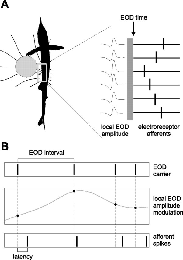
Spatial and temporal aspects of latency coding in the mormyrid electrosensory system. A, A nearby conductive object alters the pattern of current flowing through the fish’s skin at the time of the EOD (left). Object-induced changes in the LEOD amplitude are encoded by the latencies of spikes in afferents innervating neighboring electroreceptors (right). LEOD amplitude is larger for electroreceptor afferents closest to the object, resulting in shorter spike latencies. B, Pulse-type mormyrid fish emit brief EOD pulses separated by much longer intervals (top). External stimuli result in modulations in EOD amplitude sampled at the time of the EOD pulses (middle). At each electroreceptor, sequences of EOD amplitudes are encoded by sequences of afferent spike latencies (bottom).

Afferent spike latency is probably read out at the first stage of central processing in the electrosensory lobe (ELL). ELL neurons integrate precisely timed afferent input with precisely timed electric organ corollary discharge (EOCD) input linked to the motor command to discharge the electric organ (Bell, 1990a; Bell et al., 1997), and behavioral experiments show that fish can detect changes in the relative timing of afferent and EOCD signals as small as 0.1 ms (Hall et al., 1995). The simplicity and precision of the temporal code, as well as the accessibility of central mechanisms for reading the code, make the mormyrid electrosensory system an excellent one for examining the general issue of how nervous systems might use sensory information encoded in precise spike times.

The goal of the present study was to quantitatively characterize electroreceptor afferent latency coding. Using white-noise stimuli and linear filter estimation methods, we find that afferent spike latency depends on both the present EOD amplitude and on the recent history of EOD amplitudes and intervals stretching ∼100 ms into the past. We then use these models to predict afferent response to sequences of natural EOD intervals and naturalistic amplitude modulations. This analysis reveals unexpected interactions between sensing rate, the frequency of EOD amplitude modulations, and afferent encoding.

Materials and Methods

Experimental preparation.

Mormyrid fish of the species Gnathonemus petersii were used for these experiments. Fish ranged from 8 to 12 cm in length. Fish were housed in groups of 5–20, temperature was maintained at 26–28°C, and water conductivity ranged from 100 to 150 μS. Surgery was performed under metomidate anesthesia (Hypnodil; 1 mg/L) to allow for monitoring and recording of the EOD. Skin on the dorsal surface of the head was removed, and a plastic rod was cemented to the anterior part of the skull to secure the fish. The dorsal branch of the posterior lateral line nerve was exposed just behind the cranium (Bell, 1990b). On completion of the surgery, curare (10 μg/cm of body length) was given, and fresh aerated water was passed through the gills. All experiments that were performed in this study adhere to the American Physiological Society Guiding Principles in the Care and Use of Animals and were approved by the Institutional Animal Care and Use Committee of Oregon Health and Science University.

Electrophysiology.

Extracellular recordings of individual electroreceptor afferent fibers were made with glass micropipettes filled with 2 m NaCl (5–20 MΩ). Recordings of the LEOD amplitude were made using a pair of chlorided silver wires (2 mm spacing) oriented perpendicular to the skin of the fish. Spikes were digitally sampled at 20 kHz and LEOD waveforms at 100–200 kHz (CED 1401plus hardware and Spike2 software; Cambridge Electronics Design, Cambridge, UK). Data were analyzed off-line using Matlab (MathWorks, Natick, MA).

Our recordings included two distinct classes of mormyromast afferents (termed A- and B-type) that project to distinct zones in ELL (Bell et al., 1989). Whereas both A- and B-type afferents are sensitive to changes in EOD amplitude (Fig. 1), B-type afferents are also sensitive to changes in the shape of the EOD waveform (von der Emde and Bleckmann, 1992). Waveform distortions result from objects with complex impedances consisting of capacitive as well as resistive components. The present study focused exclusively on afferent encoding of EOD amplitude changes. A previous study showed that B-type afferents have low thresholds and fire four to eight spikes in response to a maximal stimulus, whereas A-type afferents have higher, more variable thresholds and fire two to four spikes in response to a maximal stimulus (Bell, 1990b). In the present study, afferents that fired at most two spikes per EOD in response to a strong stimulus were categorized as A-type and those that fired five or more spikes were categorized as B-type. However, the majority of recorded afferents responded to a strong stimulus with three or four spikes and thus could not be unambiguously categorized. We found no significant differences between A- and B-type afferents in baseline latency, interval sensitivity, or filter time constants (p > 0.05). There was a trend toward increased EOD amplitude sensitivity in B-type afferents, but this trend was not statistically significant. Although the qualitative findings of this study apply equally to A- and B-type afferents, our failure to resolve quantitative differences between the two classes could be attributable to the rather small number of afferents that could be unambiguously classified.

Electrosensory stimulation.

The naturally occurring EOD pulse, blocked by curare in our preparation, was replaced by an EOD mimic delivered via a small silver ball electrode implanted in the tail just anterior to the electric organ and a second electrode in the water just posterior to the electric organ. Digital-to-analog conversion rate for the EOD mimic was 44.1 kHz. The waveform of the EOD mimic was taken from a recording of a typical EOD waveform measured in a discharging fish anesthetized with metomidate. Metomidate does not affect either the shape or the amplitude of the EOD (Engelmann et al., 2006). For each experiment, the peak-to-peak amplitude of the EOD mimic was adjusted to match the amplitude of the fish’s own EOD measured under metomidate anesthesia. Delivering the stimulus in this way resulted in a spatial pattern of LEOD amplitude that approximately matches that produced by the naturally occurring EOD (Fig. 2A). In several fish, we compared the baseline latencies of afferent spikes evoked by the fish’s own EOD with those evoked by our EOD mimic in the same fibers (n = 14). Responses evoked by the EOD mimic were similar to those evoked by the fish’s own EOD. Differences in first spike latencies evoked by the natural EOD and by the EOD mimic ranged from 0.1 to 1 ms (mean of 0.69 ± 0.2 ms). EOD amplitude was modulated globally in all experiments. Each afferent arises from a single point on the skin surface, the electroreceptor, and electroreceptors receive no central inputs. Thus, for the purpose of recording from afferents, the spatial profiles of electrosensory stimuli can be ignored and the stimulus can be described solely in terms of modulations of global EOD amplitude. Modulations ranged from ±0.5 to 30% of the unperturbed EOD amplitude, but most of our experiments focused on the effects of small amplitude modulations (SD of <2%).

Figure 2.

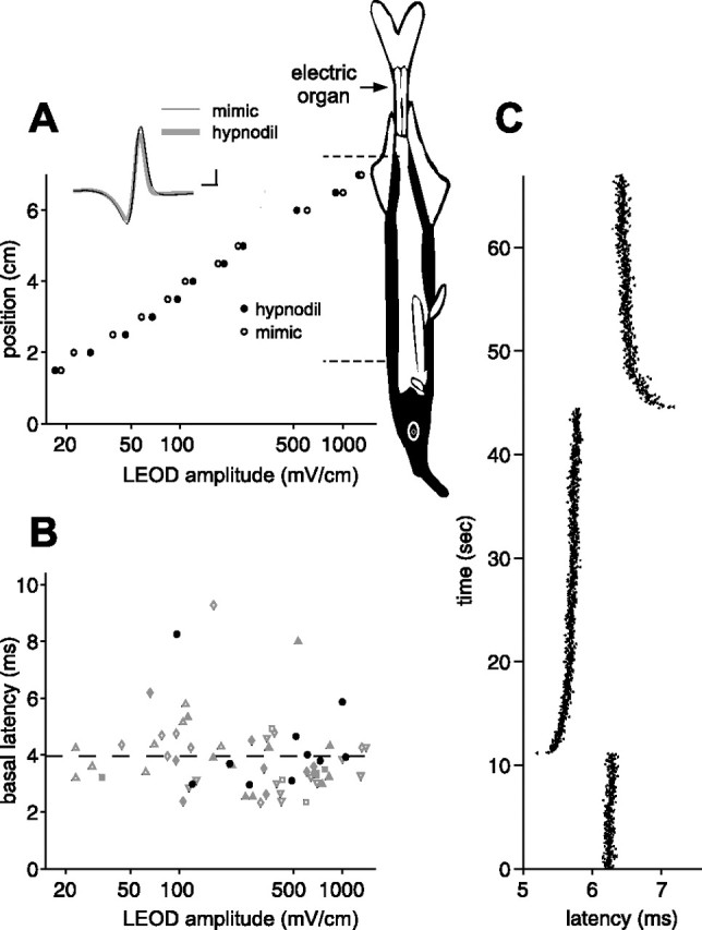
Afferent spike latency adapts to the mean EOD amplitude. A, Comparison of LEOD amplitudes measured near the skin of the fish at different rostrocaudal positions (aligned with schematic of fish). LEODs resulting from the fish’s natural discharge were similar to those resulting from our mimic. Representative LEOD waveforms are shown in the inset. Calibration: 100 mV/cm, 0.1 ms. Schematic of the fish indicates the location of the electric organ and the regions of the skin containing electroreceptors (black). Dashed lines indicate the area of the skin innervated by afferents of the posterior lateral line nerve recorded in this study. B, Differences in baseline first spike latencies in response to the EOD mimic are uncorrelated with LEOD amplitude at the receptor. Each point represents a single afferent, and different symbols represent afferents from different fish. Black circles represent afferents recorded in a naturally discharging fish. C, Adaptation in afferent first spike latency to an abrupt 5% increase followed by an abrupt 5% decrease in EOD amplitude. EOD interval was held constant at 33 ms. Note that adaptation is initially rapid and then proceeds at a much slower rate.

White-noise stimuli used for filter calculations consisted of EOD amplitudes drawn independently from a Gaussian distribution (SD of 0.5–10%) delivered at EOD intervals drawn independently from a uniform distribution (17–100 ms) or, for constant rate modulation filters, delivered at constant EOD rates (15, 30, and 50 Hz). Natural stimuli consisted of either independent EOD amplitudes or correlated amplitudes (white-noise low-pass filtered at 1 or 7.5 Hz) delivered at EOD intervals recorded in a behavioral experiment in which a fish used electrolocation to discriminate between two objects and then foraged for a food reward. The stretch of natural intervals used for these experiments was ∼22 s long. Data from 21 afferents from six fish were used for white-noise filter calculations. Recording time permitted collection of additional data for calculation of constant rate filters in three of these afferents from three fish and for responses to natural stimuli in 11 afferents from six fish.

When data were not being collected, we delivered independent EOD amplitudes and intervals to avoid long-term nonstationarities and to minimize transients at the start of data collection protocols. For filter calculations, any initial transients that remained were excluded.

Filter calculations.

To calculate linear filters for afferent spike latency, we use standard linear filter estimation methods (Marmarelis and Marmarelis, 1978; Papoulis, 1984; Rieke et al., 1997; Gabbiani and Koch, 1998), adapted to the discrete, irregularly spaced input and output of our system. We regard the input sequence of EOD pulses as the sum of two components: a “carrier” (the sequence of unperturbed EOD pulses, with fixed amplitude but variable intervals) and “modulations” (the sequence of perturbations of EOD amplitude around the mean, which vary in both amplitude and interval). Separate linear filters are assigned to carrier and modulations, and the output of the two filters is summed. Our model for afferent latency after an EOD pulse at time t is as follows:

where l₀ is the mean afferent latency, T is the set of EOD pulse times, x_c is the carrier amplitude (mean EOD amplitude), x is the modulation amplitude (deviation of EOD amplitude around the mean), K_c is the carrier filter, and K_m is the modulation filter. Minimizing mean squared error between predicted and actual latency yields a pair of coupled integral equations for the filters K_c and K_m (supplemental Methods, available at www.jneurosci.org as supplemental material). If modulation amplitudes are statistically independent of EOD intervals, these equations simplify to the following:

where C_xx is the autocorrelation of the EOD modulation amplitude, C_xl is the cross-correlation between modulation amplitude and modulations in afferent latency, M_l(u) is the conditional mean modulation in afferent latency at time t given a pulse at time t + u, and ρ(u,v) is the conditional mean rate of occurrence of pulses at time t given pulses at times t + u and t + v. We solve for the filters K_c and K_m by choosing a finite time window, discretizing time, and solving the resulting matrix-vector equations. To compute predictions using only present EOD amplitude, we take the time window to consist of time 0 alone.

In the special case in which EOD interval is constant, the recent history of EOD intervals is the same at every EOD. Hence, the carrier filter, whatever its form, will make the same contribution to afferent latency at every EOD. In that case, fluctuations in latency from EOD to EOD are attributable solely to the modulation filter, and that filter can be calculated from Equation 2 alone.

Filters are calculated using the first 90% of the data (typically 15,000–20,000 EODs) and are cross-validated by testing against the last 10%. All results and figures concerning prediction accuracy include only data from the test segment of the input, which has no overlap with the segment used to calculate the filters.

For additional discussion of the filter framework and mathematical details on filter calculations, see supplemental Methods (available at www.jneurosci.org as supplemental material).

Adjusting white-noise filters for natural intervals.

We find that a simple transformation of the filters computed for white-noise inputs is able to substantially improve predictions of afferent latency for sequences of natural EOD intervals:

where r̄ is the mean rate over the preceding 3 s, and r_wn is the mean rate for the white-noise protocol in which the original filters were calculated. The carrier filter K_c and modulation filter K_m(τ) for τ > 0 are left unchanged. The parameter λ characterizes a (hypothesized) rate-dependent scaling of sensitivity to present EOD modulation amplitude, and the parameter δ is an overall shift in latency, to account for the slower timescale effects of different mean EOD rates between white-noise and natural interval protocols. We choose λ and δ to minimize the mean squared error between actual and predicted latencies over the whole protocol (∼870 EODs). We restricted attention to cases for which filter predictions were not improved by the addition of a static nonlinearity. For these cases, the static nonlinearity can be omitted, and solving for λ and δ is a simple linear optimization problem.

Results

Electroreceptor afferent spike latency adapts to the mean EOD amplitude

We recorded unitary action potentials from mormyromast electroreceptor afferent fibers in the posterior branch of the lateral line nerve. These fibers convey information from electroreceptors on the dorsal surface of the trunk and tail to the first stage of electrosensory processing in ELL (Bell and Russell, 1978). The stimulus was a brief (0.2 ms) electrical pulse that mimicked both the temporal waveform and the spatial pattern of current flow characteristic of the fish’s own EOD (n = 7 fish) (Fig. 2A). Use of the artificial stimulus allowed us to control the intervals between EOD pulses and thus mimic the fish’s sensing behavior. For all of the experiments described in this paper, EOD amplitude was modulated globally. LEOD modulations that drive electroreceptor afferents are proportional to this global modulation (1% global modulation yields 1% LEOD modulation). We found that LEOD amplitude, whether generated by the fish itself or by our mimic, falls off steeply with distance from the electric organ, consistent with modeling studies (Caputi and Budelli, 1995) (Fig. 2A). For a subset of recorded afferents, we located the electroreceptor pore and measured the LEOD. We found no significant correlation between the unperturbed LEOD amplitude and first spike latency (p > 0.2 both across the population and within each fish) (Fig. 2B), despite a >30-fold reduction in LEOD amplitude from the tail to the head, suggesting that afferents are capable of adapting to a wide range of LEOD amplitudes. Such adaptation is readily observed after abrupt changes in EOD amplitude (Fig. 2C). The adaptation consists of a fast initial phase of a few seconds or less, followed by a slow phase lasting minutes. Adaptation of this type was observed in nearly all afferents tested but was not investigated systematically in this study.

Electroreceptor afferent first spike latency depends on EOD amplitude and sensing intervals

Previous studies have noted the rather remarkable dependence of electroreceptor afferent spike latency on EOD amplitude (Fig. 3A) (Szabo and Fessard, 1965; Szabo and Hagiwara, 1967; Bell, 1990b; Gomez et al., 2004). Increases in EOD amplitude result in smooth decreases in afferent spike latency of up to 10 ms, with a timing jitter on the order of 0.1 ms or less.

Figure 3.

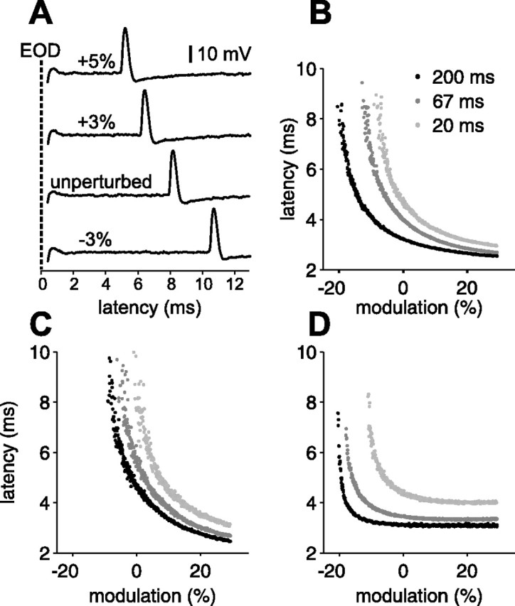
Afferent spike latency depends on EOD amplitude and sensing behavior. A, Representative extracellular traces illustrating the shift in afferent spike latency resulting from changes in EOD amplitude. The interval between EODs was 67 ms. B–D, Smooth ramps in EOD amplitude at three constant EOD intervals (200, 67, and 20 ms) for three different afferents. Increases in EOD amplitude result in smooth decreases in afferent first spike latency. The shorter the EOD interval, the longer the latency for a given amplitude.

The goal of the present study was to characterize afferent encoding in the context of varying sensing interval patterns and modulations of EOD amplitude typical of small objects or prey. As a first step in this direction, we recorded afferent response to smoothly ramped EOD amplitude modulations. For each afferent, EODs were delivered at three constant intervals (200, 67, and 20 ms). At each interval, amplitude modulation ramped linearly from −30 to +30% over 900 EODs. Ramps at long, medium, and short intervals were delivered successively. Results from three afferents are shown in Figure 3B–D. For clarity, only the first spike latency is plotted. Several lines of evidence suggest that the first spike is the sole effective degree of freedom in the afferent response (Bell, 1990a,b; Gomez et al., 2004). Additional experiments supporting this idea are described below (see Fig. 5). Several features were common to all afferents tested (n = 18). As described previously, latency was a decreasing monotonic function of EOD amplitude (Szabo and Fessard, 1965; Szabo and Hagiwara, 1967; Bell, 1990b). Both the sensitivity (the change in latency for a given change in EOD amplitude) and jitter (the SD of the latency for a given amplitude) increase at the long end of the latency range. We also found that shorter EOD intervals resulted in longer latencies for a given EOD amplitude, clearly indicating that the sensing behavior of the fish affects afferent stimulus encoding.

Figure 5.

Subsequent spikes in the afferent response do not carry additional information. A, Mean second spike latency versus mean first spike latency for a putative A-type afferent. Each point is based on responses to a different stretch of random EOD amplitudes and sensing intervals. Error bars are SEMs. B, Mean second and third spike latency (black and gray, respectively) versus mean first spike latency for a putative B-type afferent. In both A and B, subsequent spike latencies appear to be simple functions of (i.e., are correlated with) first spike latency.

We also observed differences across afferents. The shape and position (i.e., baseline latency) of the latency–amplitude curve as well as its slope at the unperturbed EOD amplitude varied substantially across afferents. The effects of interval also vary across afferents, in both their overall magnitude and their relative magnitude at different latencies (Fig. 3, compare B–D).

To verify that significant changes in afferent spike latency occur as a consequence of natural sensing behavior, we delivered a constant EOD amplitude at intervals recorded in a behavioral experiment in which a fish used electrolocation to discriminate between two objects and then foraged for a food reward (Fig. 4A). In all afferents tested (n = 20), afferent spike latency was clearly sensitive to these natural interval fluctuations, shifting later as the EOD interval decreased (Fig. 4B). In absolute terms, these shifts appear small (typically <2 ms), but, relative to the precision of the afferent latency code (on the order of 0.1 ms or less), they are surprisingly large.

Figure 4.

Effects of natural sensing intervals on afferent spike latency. A, EOD intervals recorded in a behavioral experiment in which a fish discriminated between two objects and then foraged for food. Intervals were short and regular during probing (bracket) and longer and irregular during foraging. B, Afferent first spike latency evoked by a constant EOD amplitude delivered at the natural EOD intervals shown in A. Latency clearly depends on the previous intervals, increasing as EOD interval decreases. D, Latency shifts evoked by small transient increases in EOD amplitude (shown in C) are clear when sensing interval is approximately constant (open rectangle) but can be obscured when sensing intervals vary (shaded rectangle). EOD intervals are the same as shown in A.

As a point of comparison, we measured the latency changes induced by small (1.5%), transient increases in EOD amplitude (Fig. 4C) delivered in the context of the same natural interval patterns. These transients are comparable with or larger than EOD modulations caused by invertebrate prey (Nelson and MacIver, 1999; Chen et al., 2005). When EOD intervals are approximately constant, decreases in latency induced by the transient stimulus are clearly visible (Fig. 4D, open rectangle). However, when EOD intervals are irregular, latency shifts attributable to variations in sensing intervals obscure latency shifts caused by the stimulus (Fig. 4D, shaded rectangle). These findings are especially intriguing because variable sensing interval patterns are typical of foraging behavior in mormyrid fish (von der Emde, 1992).

The dependence of afferent output on both EOD amplitude and sensing intervals seems to present a decoding problem for central neurons in ELL. These neurons must extract information about changes in the local EOD amplitude attributable to nearby objects from afferent spike latencies that also depend on the fish’s behavior. Regardless of how LEOD amplitude is extracted by downstream neurons, our initial results suggest that an analysis of afferent encoding must treat EOD amplitudes and sensing intervals jointly, asking how each contributes to afferent output.

Afferent output often consists of a brief burst of spikes, so an important initial question was whether the second and subsequent spikes are simply locked to the first spike or whether they are independent degrees of freedom that may carry additional information. We addressed this question by examining afferent response to ∼100 repeats of a 6 s stretch of random EOD amplitudes delivered at random EOD intervals spanning most of the natural interval range (17–100 ms). We compared mean latency of subsequent spikes with mean latency of the first spike, for EODs with identical interval and amplitude histories. Each EOD evoked one to four spikes in these experiments, as is typical of mormyromast afferents. As expected, larger EOD amplitudes and longer EOD intervals led to shorter spike latencies and more spikes per EOD. The latency (n = 10) (Fig. 5), probability, and number (data not shown) of subsequent spikes were simple monotonic functions of the first spike latency. Thus, although EOD amplitude and EOD interval both drive afferent output, the timing of a single spike appears to be the sole encoding variable. In light of these results, our subsequent analysis focused exclusively on the first spike in the afferent response.

Linear filter analysis of electroreceptor afferent encoding

Although initially surprising, a dependence of afferent spike latency on previous EOD intervals is consistent with the common finding that neurons integrate their inputs over some stretch of the recent past. A general mathematical framework for characterizing such input–output relationships is the Volterra or Wiener functional expansion (Volterra, 1930; Wiener, 1958; Marmarelis and Marmarelis, 1978; Rieke et al., 1997). This is a black-box approach that does not rely on any knowledge of underlying physical mechanism. For input–output relationships that are approximately linear, only the first two terms in this expansion, the zeroth order (mean) and the first order (linear filter) terms, are needed to obtain useful predictions of the output of the system. Such linear filter models, either alone or in combination with a static nonlinearity (Hunter and Korenberg, 1986; Chichilnisky, 2001), have been widely deployed to model the instantaneous firing rate of neurons as a function of their recent history of stimulus input (Sakai, 1992).

Suitably adapted to the discrete, irregularly spaced input and output of our system, a linear filter framework could provide a useful tool for quantitatively characterizing the joint dependence of afferent spike latency on EOD amplitude and preceding intervals, provided this dependence is approximately linear. Linearity in this setting means, for example, that the latency shift caused by the combination of a change in present EOD amplitude and the occurrence of a previous EOD at a certain interval should be approximately the sum of the latency shifts caused by each of these alone. Similarly, the latency shift caused by two previous EODs should be approximately the sum of the shifts caused by each previous EOD alone.

As an initial test of linearity, we examined data from white-noise experiments in which both EOD amplitude and sensing intervals were varied randomly. Histograms in Figure 6A show distributions of first spike latency for a representative afferent for four different stimulus histories, in which the only EODs occurring within the previous 80 ms were as follows: no previous EOD within 80 ms (baseline); one previous EOD, 17–32 ms before the present; one previous EOD, 32–47 ms before the present; and two previous EODs, one 17–32 ms before the present and one 32–47 ms before the present. Mean latency is indicated by the vertical lines. Single previous EODs each separately increase afferent spike latency relative to baseline, and the effect of both together is close to the sum of the effects of each separately (Fig. 6B). Similarly, histograms in Figure 6C show distributions of first spike latency for the same afferent under the following four conditions: no previous EOD within 80 ms (baseline); present EOD amplitude larger than the mean (0.1–0.5% modulation); one previous EOD, 17–32 ms before the present; and present EOD larger than the mean and one previous EOD, 17–32 ms before the present. An increase in EOD amplitude causes a latency decrease, whereas a previous EOD results in a latency increase. The effect of both together is again close to the sum of the effects of each separately (Fig. 6D).

Figure 6.

Approximate linear summation of effects of previous EOD intervals and present EOD amplitude. A, Histogram of latencies for the following (top to bottom): no previous EOD within 80 ms (baseline); one previous EOD, 17–32 ms before the present (1); one previous EOD, 32–47 ms before the present (2); and two previous EODs, one 17–32 ms before the present and one 32–47 ms before the present (both). Mean latency indicated by vertical line. B, Change in mean latency from baseline, for conditions 1, 2, and both, and the linear sum of 1 and 2 (sum). Error bars are SEMs. C, Histogram of latencies for the following (top to bottom): no previous EOD within 80 ms (baseline); present EOD amplitude larger than the mean (0.1–0.5% modulation) (1); one previous EOD, 17–32 ms before the present (2); and present EOD larger than the mean and one previous EOD, 17–32 ms before the present (both). D, Change in mean latency from baseline, for conditions 1, 2, and both, and the linear sum of 1 and 2 (sum). Data in A–D are from a representative afferent. E, Linearity ratios (see Results) for the effects of two previous EODs for 18 afferents. F, Linearity ratios for the effects of present EOD amplitude and previous EOD for the same afferents as in E, excluding those for which the effects of 1, 2, or sum were not statistically significant (p > 0.05). Gray lines indicate ±10% deviation from linearity, and dashed lines indicate ±20% deviation from linearity.

These same comparisons were made with several other pairs of previous intervals or present amplitude and previous interval, and results were consistent with those shown. We define the linearity ratio to be the ratio of the effect of both previous EODs (or both present amplitude and previous EOD) to the sum of the effects of each separately; for perfect linearity, this ratio would be 1. For the effects of two previous EODs, 16 of 18 afferents were within 20% of linearity, and 10 of 18 were within 10% (Fig. 6E). For the effects of present amplitude and one previous EOD, 13 of 13 were within 20% of linearity, and 9 of 13 were within 10% (Fig. 6F). Because most of the afferents we tested were approximately linear by these simple direct tests, an application of linear filter methods seems well justified. Note that this analysis also shows that afferent spike latency depends on previous intervals beyond the first.

To adapt the standard linear filter framework to the active electrosensory system of a pulse-type fish, we regarded the input sequence of EOD pulses as the sum of two components: a carrier (the sequence of unperturbed EOD pulses, with fixed amplitude but variable intervals) and modulations (the sequence of perturbations of EOD amplitude around the mean, which vary in both amplitude and interval) (Fig. 7A). Separate linear filters are calculated for the carrier and the modulations; predicted afferent latency is the summed output of the two filters (additional details on the filter model and filter calculations are provided in supplemental Methods, available at www.jneurosci.org as supplemental material). The carrier contribution is the effect of the fish’s sensing interval behavior alone; the modulation contribution is the effect of the external world, sampled at the discrete times of the carrier pulses.

Figure 7.

Relative contributions of EOD amplitude and sensing intervals to afferent output revealed by a linear filter analysis. A, Schematic illustrating input to the electrosensory system as a carrier plus modulations. The temporal characteristics of the carrier are not fixed as the sequence of EOD intervals varies. B, F, Carrier and modulation filters for first spike latency for two different afferents, computed from experiments in which EODs were delivered at independent intervals (17–100 ms) with independent Gaussian amplitude modulation SDs of 1% (B) and 5% (F) of the unperturbed EOD amplitude. Sensitivity to present EOD amplitude modulation is indicated by the black circle. Sensitivity to past amplitude modulations is indicated by the black curve. Sensitivity to previous intervals is indicated by the gray curve. Aggregate sensitivity to all previous intervals is indicated by gray circle. Filters are not defined in gray region in which no EODs occur. E, Static nonlinearity mapping filter output onto predicted latency, for the afferent in F. C, G, Actual first spike latency versus latency predicted by the linear filters in B and F. D, H, Actual versus predicted first spike latency based on the present EOD amplitude alone.

Linear filters and filter predictions for two afferents are illustrated in Figure 7. In one case, the EOD amplitude modulation was small (1% SD; top panels), and, in the other, the amplitude modulation was large (5% SD; bottom panels). The value of the modulation filter at time τ is the sensitivity of afferent latency to modulations of the amplitude of an EOD pulse at time τ before the present, and the value of the carrier filter at time τ is the sensitivity to the presence of a pulse (of mean amplitude) at time τ before the present. For this protocol, no EOD intervals fell in the range 0–17 ms, so the filters are not defined for those values of τ (Fig. 7B,F, gray rectangles). The filter values at time τ = 0 have a special status in this system: the modulation filter at time 0 is the sensitivity to modulations in present EOD amplitude, and the carrier filter at time 0 can be shown to be the aggregate sensitivity to all previous intervals, i.e., the mean shift in latency that would result if all previous EODs were removed (supplemental Methods, available at www.jneurosci.org as supplemental material). For plotting purposes, the carrier filter is given in units of milliseconds per pulse, and the modulation filter is given in milliseconds per 1% amplitude modulation.

For both afferents in Figure 7, the qualitative form of the linear filters is consistent with previous observations. Sensitivity to present EOD amplitude (modulation filter at time τ = 0) (Fig. 7B,F, black circle) is negative in sign, indicating that higher EOD amplitude leads to shorter latency. Sensitivity to previous intervals (carrier filter for τ > 0) (Fig. 7B,F, gray curve) is positive and monotonically decreasing, indicating that shorter EOD intervals lead to longer latency. Sensitivity to past EOD amplitudes (modulation filter for τ > 0) (Fig. 7B,F, black curve) is substantially smaller than sensitivity to present amplitude and is opposite in sign, so that higher EOD amplitudes in the past lead to longer latency. When EOD amplitude modulations were large (SD of 5% of the unperturbed EOD amplitude or larger), we observed compression at the short end and expansion at the long end of the latency range (visible as curvature in Fig. 3B–D). In such cases, the linear filters were supplemented with a static nonlinearity (Hunter and Korenberg, 1986; Chichilnisky, 2001), mapping filter output onto predicted latency (Fig. 7E) (supplemental Methods, available at www.jneurosci.org as supplemental material). Predictions with and without a static nonlinearity are shown in supplemental Figure 1 (available at www.jneurosci.org as supplemental material) (same afferents as in Fig. 7).

For large amplitude modulations, afferents were often driven through a large fraction of their dynamic range. In such cases, the filter model (with accompanying static nonlinearity) can be regarded as an approximation to the global input–output relationship of the afferent. For small amplitude modulations, afferents were driven through only a small fraction of their range; the linear filters are then properly thought of only as local approximations to the global input–output relationship.

Prediction accuracy can be quantified by the coefficient of determination (r²) between predicted and actual latency, which measures how much of the variance in actual latency is captured by a linear relationship with the prediction. To assess the importance of the past (previous EOD intervals and amplitudes), we compare predictions using the full filters with predictions using present EOD amplitude alone [in which we recompute filters on the time window consisting of time 0 alone (supplemental Methods, available at www.jneurosci.org as supplemental material)]. For both afferents shown in Figure 7, the full filter prediction captures more than 90% of the variance in actual latency (Fig. 7C,G). For the afferent driven by large (5% SD) amplitude modulations, we do almost as well using only present EOD amplitude (Fig. 7H), but, for the afferent driven by small (1% SD) amplitude modulations, we do only about half as well (Fig. 7D). The past is less important for large amplitude modulations than for small because of differences in the relative contributions of present EOD amplitude and past intervals. Contributions from present amplitude modulation scale with the size of the modulation, whereas contributions from the carrier filter do not.

Collective results of our filter analysis are summarized in Figure 8(21 afferents from six fish). The SD of EOD amplitude modulations ranged from 0.5 to 10%. A limited recording time allowed us to test only one amplitude SD for each afferent. We found the qualitative form of the filters to be highly consistent across afferents. Sensitivity to present EOD modulation amplitude was always negative (higher amplitude leads to shorter latency); sensitivity to previous intervals was always positive (previous EODs lead to longer latency) and monotonically decreasing with time before the present (shorter EOD intervals increase latency more than longer intervals) (Fig. 8A). Sensitivity to amplitude modulations in the past was always substantially smaller than sensitivity to present EOD amplitude, thus our estimates of the modulation filter for τ > 0 were noisy (Fig. 8B). Nevertheless, they too were qualitatively consistent across afferents, with sensitivity to past amplitudes tending to have opposite sign to sensitivity to present amplitude (higher amplitudes in the past lead to longer latency) and tending to decrease with increasing time before the present. The decay of both the carrier (Fig. 8A, inset) and past modulation filters is approximately exponential. It is interesting to note that the opposite character of present and past amplitude sensitivities is similar to the biphasic form of linear filters in other systems (Sakai, 1992).

Figure 8.

Collective data for white-noise filters. A, Overlay of carrier filters for all afferents tested. Inset, Carrier filters show roughly exponential decay. B, Overlay of modulation filters for past modulations for all afferents tested. C, Histogram of aggregate interval sensitivities. D, Histogram of present amplitude sensitivities. E, Coefficient of determination (r²) between actual and predicted first spike latency versus size of amplitude modulation. F, Relative importance of the present EOD amplitude (ratio of r² for the prediction using present EOD alone to that for the prediction using present and past) versus size of modulation amplitude. For modulation SDs of ∼1–2% of the unperturbed EOD amplitude, present and past are comparable in importance.

Despite an overall similarity in qualitative form, there were significant quantitative differences across afferents for some filter parameters. Aggregate sensitivity to previous intervals ranged from 0.1 to 0.3 ms (n = 21) (Fig. 8C), and sensitivity to present EOD amplitude ranged from 0.03 to 0.4 ms per 1% modulation (n = 21) (Fig. 8D). Interval sensitivity was correlated with baseline latency (r = 0.54; p = 0.01), as was amplitude sensitivity (r = 0.43; p = 0.05). Interval and amplitude sensitivity were not significantly correlated with each other (p > 0.2). Carrier and modulation filters were fitted with exponential functions. There was no significant correlation between time constants for carrier and modulation filters in the same afferent or between filter time constants and interval sensitivity, amplitude sensitivity, or baseline latency (p > 0.3). The time to fall to 5% of maximum value (three time constants) was 102 ± 28 ms (mean ± SD) for the carrier filters and 109 ± 76 ms for the modulation filters. Thus, the response to the present EOD is influenced by the recent history of EOD intervals and amplitudes extending ∼100 ms into the past.

Filter predictions were quite accurate across a range of modulation amplitudes (Fig. 8E), with coefficients of determination above 0.9 for a number afferents. As discussed above, the relative importance of the past was clearly a function of the size of EOD amplitude modulations. For large amplitude modulations, the present EOD amplitude dominates, whereas for small EOD amplitude modulations (SD of 1–2% or less), predictions that take the recent history of EOD amplitudes and intervals into account are substantially better than predictions using present EOD amplitude alone (Fig. 8F). These results confirm the significant effects of sensing behavior on afferent spike latency under conditions in which sensing intervals are irregular (as is typical of foraging) and EOD amplitude modulations are small (as expected for prey).

Electroreceptor afferent encoding in the context of natural inputs

Linear filters provide a concise description of how present EOD amplitude, past EOD amplitudes, and past sensing intervals contribute to afferent spike latency in the context of white-noise (statistically independent) inputs. However, the statistics of natural sensing behavior are characterized by temporal structure (correlations) on multiple timescales. For example, fish transition abruptly from periods of brief, highly regular intervals to periods of longer more irregular intervals (Fig. 4A). LEOD amplitude modulations in a swimming fish would also be characterized by correlations on multiple timescales, resulting from movement of the fish, boundary conditions, and foreground objects (Chen et al., 2005). Our next series of experiments were aimed at gaining some initial insight into how natural patterns of sensing behavior and correlated EOD amplitude modulations affect afferent encoding.

For a subset of afferents for which we computed white-noise filters, we also delivered a sequence of natural intervals (Fig. 4A), with three types of amplitude modulation: independent, white-noise low-pass filtered at 7.5 Hz (and sampled at the time of occurrence of the EOD), and white-noise low-pass filtered at 1 Hz. Both correlated modulations are within the frequency range expected for natural EOD amplitude modulations. The size of the amplitude modulations ranged from 0.5 to 3.3% SD. We compared actual responses for natural sensing interval patterns and correlated EOD amplitude modulations with those predicted by white-noise filters for the same afferents (Fig. 9A). White-noise filters were supplemented with a static nonlinearity in 6 of the 11 afferents (gray symbols). For all 11 afferents, accuracy of white-noise filter predictions was highest for independent intervals and independent amplitude modulations (*), lower for natural intervals and independent amplitude modulations (+), and lowest for natural intervals and 1 Hz correlated amplitude modulations (□). The prediction accuracy for 7.5 Hz correlated amplitude modulations was slightly less than for independent modulations (data not shown). Actual versus predicted latency for a representative afferent is shown in Figure 9B–D. Loss of prediction accuracy was especially evident for 1 Hz correlated amplitudes at the long end of the latency range (Fig. 9D, arrow), where the range of predicted latencies was much smaller than the range of actual latencies.

Figure 9.

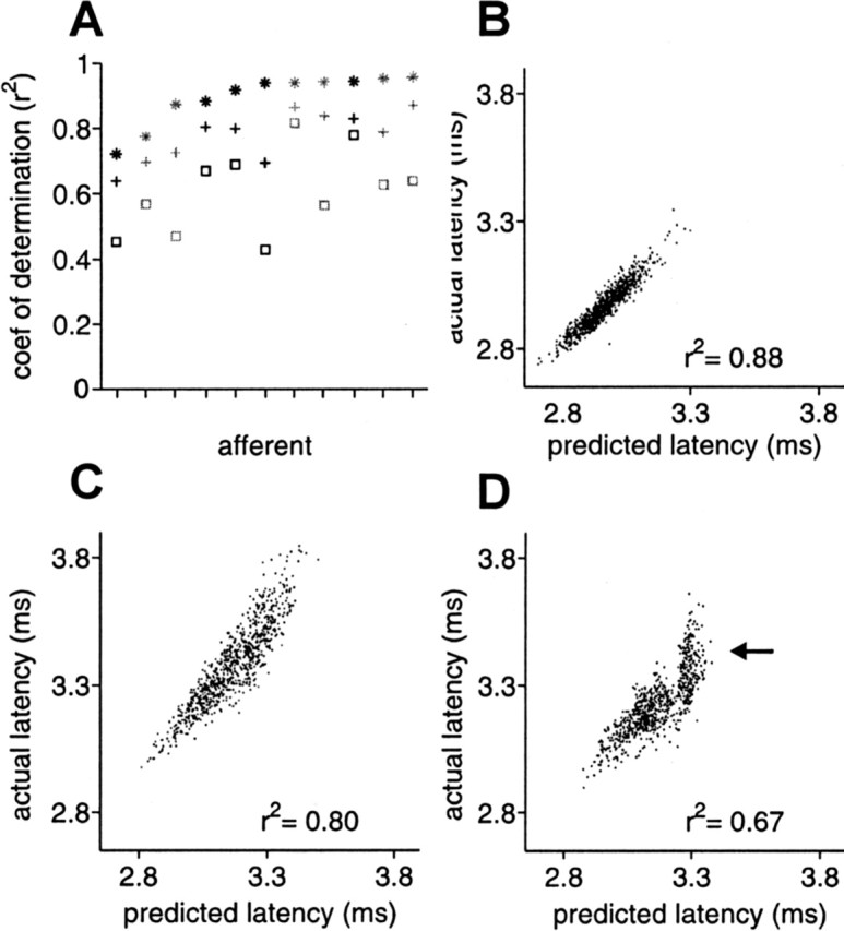
White-noise filters are partially successful in predicting response for natural EOD intervals. A, For 11 afferents, coefficient of determination between actual latency and latency predicted by white-noise filters, for independent intervals and independent amplitude modulations (*), for natural intervals and independent amplitude modulations (+), and for natural intervals and correlated (low-pass filtered at 1Hz) amplitude modulations (□). Gray symbols indicate filters augmented with a static nonlinearity. Prediction accuracy is lower for natural intervals and for correlated amplitude modulations. The natural interval sequence used in these experiments is shown in Figure 4A. B–D, Actual versus predicted latency in an example afferent, for independent intervals and independent amplitudes (B), natural intervals and independent amplitudes (C), and natural intervals and correlated amplitudes (D).

Note that most of these longer latencies are attributable to the stretch of high regular rate that occurred while the fish was actively probing objects (Fig. 4A, bracket). In addition to increases in latency expected on the timescale of the carrier filters, sustained high EOD rates result in additional increases in latency on slower timescales (Figs. 4B, bracket) (see Fig. 11F, 50 Hz). The mean EOD rate for the natural interval sequence was substantially higher than for the white-noise experiments, and both rapid and slower timescale effects of rate are evident as systematic offsets in Figure 9, C and D. The expected latency increase attributable to the carrier filter is reflected in the mean predicted latency for natural intervals (Fig. 9C,D) being longer than mean predicted latency for independent intervals (Fig. 9B). The additional slower timescale increase in latency is evident in the mean actual latency for natural intervals being longer than predicted (Fig. 9C,D).

Figure 11.

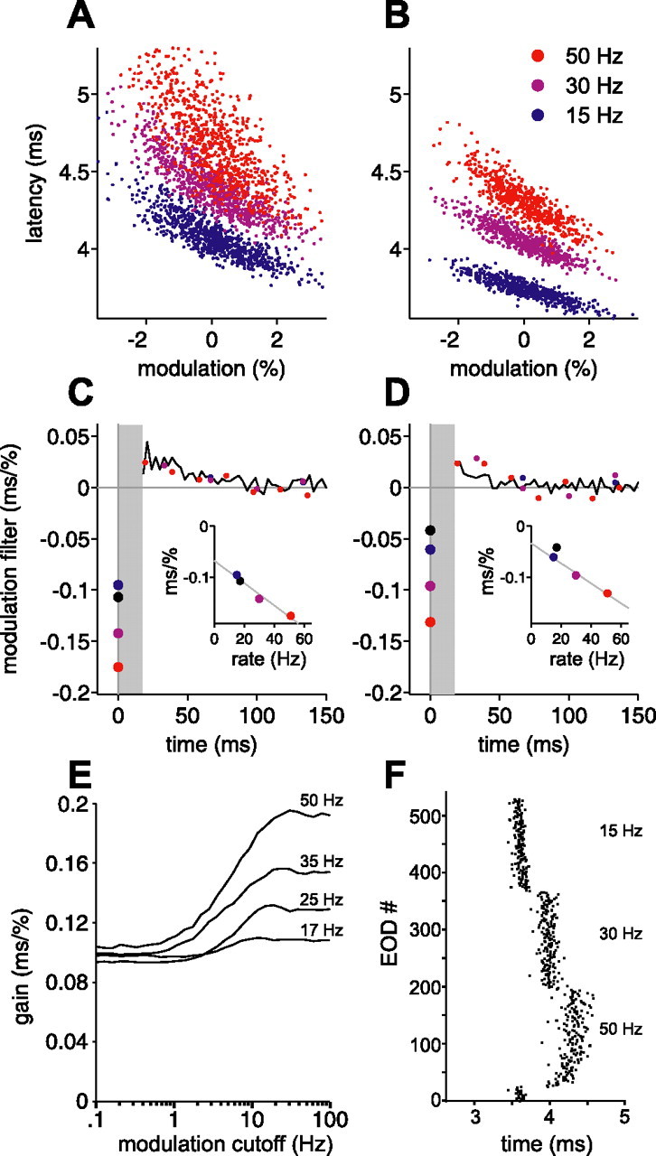
Sensitivity to present EOD amplitude increases linearly with constant EOD rate. A, B, Actual latency versus present EOD modulation amplitude for two afferents, at constant EOD rates of 15 Hz (blue), 30 Hz (purple), and 50 Hz (red), for independent amplitude modulations. Note the steeper slope (gain) at higher rates. C, D, Modulation filters for the afferents in A and B, for these three constant intervals. Modulation filters for independent intervals for the same afferents are shown in black. Sensitivity to present amplitude modulation (circles at time 0) increases approximately linearly (insets) with increasing rate. Gray line in insets is a least-squares fit to the three constant-interval sensitivities. E, Calculated gain versus low-pass cutoff frequency of correlated amplitude modulations, for the white-noise modulation filter of the afferent in A and C with present amplitude sensitivity scaled according to the relationship in C, inset. Longer correlation times (lower cutoff frequencies) still lead to a loss of gain at all rates, but the loss at higher rates is no worse than at lower rates; compare with Figure 10H, which is based on the white-noise filter for the same afferent. F, A portion of the protocol used for the afferent in B. Note the longer mean latencies at higher rates, with both rapid and slower phases of drift after a change in rate. Only the second half of each constant-rate block was used for analysis.

To better understand the respective effects of natural sensing intervals and amplitude correlations, we looked more closely at the discrepancies between actual and predicted latency for these experiments. Figure 10 shows predicted latency (A, C) and actual latency (B, D) versus modulation amplitude, for independent modulations (A, B), and for 1 Hz correlated modulations (C, D), for the same natural interval sequence in a single afferent. Blue points indicate EODs for which the instantaneous EOD rate (the reciprocal of previous interval) was below 30 Hz. Red points indicate EODs from the stretch of high regular rate (49–54 Hz) that occurs while the fish was actively probing objects (Fig. 4A, bracket). Overlaid lines are least-squares regression lines through the correspondingly colored data points. The magnitude of the slope of such a line is a measure of “overall” sensitivity to EOD amplitude. To avoid confusion between this overall sensitivity and sensitivity to any single modulation amplitude, we refer to the former as “gain.” For correlated amplitude modulations, gain for latency predicted by the white-noise filters is reduced at high EOD rate compared with low rate (Fig. 10C). This effect was observed in 10 of 11 afferents tested (p < 0.05, one-tailed z test). This decrease in gain is not evident in the actual latency (Fig. 10D). In fact, actual gain was significantly higher at high EOD rates in 9 of 11 afferents.

Figure 10.

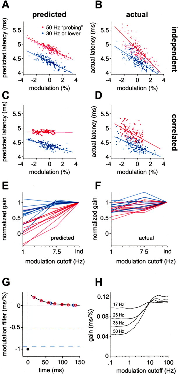
Discrepancies between actual and predicted latency for natural intervals and correlated amplitudes suggest a relationship between sensing rate, frequency of amplitude modulation, and afferent gain. A, B, Predicted (A) and actual (B) latency versus modulation amplitude, for natural intervals and independent amplitudes, with points colored by instantaneous rate. Actual latency has greater amplitude gain (magnitude of slope) at higher rates (red), whereas predicted latency has roughly constant gain. C, D, Same as A and B, but for correlated amplitudes. Actual latency (D) shows roughly constant amplitude gain at different rates, whereas predicted latency (C) shows markedly lower gain at high rates. E, F, Normalized gain versus cutoff frequency of correlated amplitude modulations (1 Hz, 7.5 Hz) at low EOD rate (blue) or high EOD rate (red), for predicted latency (E) and actual latency (F), in 11 afferents. Gains are normalized by gain for independent (ind) modulations in the same afferent. For plotting purposes, ind is placed at 30 Hz, just above the Nyquist frequency for EOD intervals used. G, Schematic explanation for the loss of gain in predicted latency in C. If the correlation time of amplitude modulations is much greater than the filter width, then modulation amplitude is roughly constant over the filter window. Present and past modulation amplitudes then make opposing contributions to latency. The summed effects of past and present modulations at low rate (blue circles) lead to a small loss of gain, but, at high rate (red circles), the loss may be substantial. Values for the respective gains are indicated by dashed lines. H, Calculated gain versus low-pass cutoff frequency of correlated amplitude modulations, for constant rates of 17 (mean rate for white-noise protocol), 25, 35, and 50 Hz, using the white-noise modulation filter for the afferent shown in A–D. Longer correlation times (lower cutoff frequencies) lead to a loss of gain at all rates, but the loss is greater at higher rates.

The relationship between predicted gain and modulation cutoff frequency is summarized for the same 11 afferents in Figure 10E. Predicted gain was significantly lower for 1 Hz correlated than for independent amplitude modulations in 9 of 11 afferents at low rate (blue lines) and in 11 of 11 afferents at high rates (red lines) (p < 0.05, one-tailed z test). Although actual gain also decreases with increasing amplitude correlation (Fig. 10F), the relative magnitude of this decrease is substantially less than predicted. This discrepancy is particularly clear at high EOD rates, in which normalized gain for 1 Hz correlated amplitudes was significantly less for predicted than for actual latency in 10 of 11 afferents.

Both the rate- and correlation-dependent loss of gain in the white-noise prediction could have been anticipated from our linear filter analysis. Their explanation is illustrated schematically in Figure 10G. Black curve and black circle represent a typical (idealized) modulation filter. If amplitude modulations are highly correlated over the width of the modulation filter, contributions to latency from past modulations add up in a consistent way, in a direction that opposes the contribution from the present EOD modulation. The gain is the sum (per unit amplitude) of the contributions of past and present EOD amplitude modulations. At low EOD rates (blue circles), the resulting loss of gain is small (blue dashed line), but, for high rates (red circles), the loss can be substantial (red dashed line). This is consistent with the substantially lower gain (magnitude of slope) at high rate in Figure 10C. In contrast, if amplitude modulations are uncorrelated, past modulations will make statistically independent contributions (some negative and some positive), which will tend to cancel each other out, and gain will be only slightly affected by rate. This is consistent with the roughly equal gains in Figure 10A. These are two very different outcomes, but the filter is the same in both cases; the difference is in the correlation structure of the input and in the rate at which that input is sampled.

We calculated the expected effects of amplitude correlations and sampling rate on gain for the measured white-noise modulation filter of the afferent shown in Figure 10A–D. In Figure 10H, we plot predicted gain versus modulation cutoff frequency (low-pass, fourth-order Butterworth) for constant EOD rates of 17 (mean rate for independent intervals), 25, 35, and 50 Hz. From these curves, we can infer the effects of rate at a given amplitude correlation. For independent modulations (high cutoff frequency), predicted gain varies only mildly with rate, as seen in Figure 10A. For modulations highly correlated over the ∼100 ms width of the filter (cutoff frequencies of ∼2 Hz or less), predicted gain falls substantially with increasing rates. For a cutoff frequency of 1 Hz, gain at an EOD rate of 50 Hz is down by almost 60% compared with 17 Hz and 40% compared with 25 Hz, in qualitative agreement with Figure 10C. This is not at all consistent with the actual gain in Fig 10D, which appears to be roughly independent of rate.

One possible explanation for the discrepancies between actual and predicted gains is that the higher overall mean rate of the natural interval sequence (compared with white-noise intervals), or stretches of sustained high rate within the natural interval sequence, induce changes in the modulation filter for actual latency.

To test this possibility directly, we computed modulation filters, using independent amplitude modulations, for three constant EOD rates. Actual latency versus modulation amplitude at each rate is shown in Figure 11, A and B; note the increase in gain with increasing rate. Filters for 15 Hz (blue), 30 Hz (purple), and 50 Hz (red) are shown overlaid on the modulation filter for independent intervals and amplitudes in the same afferent (black) (Fig. 11C, D). The protocol consisted of repeated short blocks of 180 EODs at each rate (3.6 s at 50 Hz, 6 s at 30 Hz, and 12 s at 15 Hz). After an increase in EOD rate, afferent spike latency moved later, with an initial rapid phase and a subsequent slower phase (Fig. 11F). To minimize the influence of these nonstationarities after changes in rate, filters were calculated using only the second half of each block. Modulation filters under these conditions change with rate in a particularly simple way: sensitivity to present modulation amplitude increases roughly linearly with EOD rate (Fig. 11C, D, inset). This is consistent with the increases in gain in Figure 11, A and B, and is also consistent with previous results: increases in EOD rate result in longer latencies in which sensitivity to EOD amplitude is higher (Fig. 3B–D). Because the linear filters in Figure 11 are local approximations, the changes we observe may simply be a consequence of longer mean latency at higher EOD rate, coupled with fixed global filters and a fixed global static nonlinearity whose slope increases at longer latency. However, in this case, one would also expect rate-dependent changes in the local modulation filter in the past, which are not evident in our data. Alternatively, changes in local filters may reflect rate-dependent changes in the global input–output relationship.

Regardless of mechanism, the observed changes in sensitivity provide a clear means for sensing behavior to influence afferent gain. For correlated modulations, an increase in present amplitude sensitivity could in principle counteract the opposing effects of past modulations depicted in Figure 10E. This may explain (assuming that such changes are also induced by natural interval sequences) how actual latency is able to maintain gain for correlated modulations at high EOD rates (Fig. 10D). We calculated the expected gain for the white-noise modulation filter (Fig. 11E), this time taking into account the rate dependence of sensitivity to present amplitude modulation observed in the constant-rate modulation filters (data in the left column of Fig. 11 are from the same afferent as Fig. 10). For independent modulations (high cutoff frequency), gain is now higher at higher rates. For slow correlated modulations (cutoff of ∼2 Hz or less), the increase in present amplitude sensitivity opposes the effects of past amplitudes, so that gain, instead of being lower at high rate, is actually higher at high rate. This is in qualitative agreement with the actual gains that we observe in Figure 10, B and D.

Although our data do not allow us to directly calculate modulation filters at different points in the sequence of natural intervals, it seems reasonable to take the above findings one step further by asking whether the predictions of white-noise filters for natural intervals and 1 Hz correlated modulations (Fig. 9A, squares) can be “rescued” by incorporating the interval-dependent sensitivity scaling observed above. We attempt to do this by transforming the white-noise modulation filter as it appears to be transformed in Figure 11, C and D, but using the mean rate over the preceding 3 s of natural intervals, instead of a constant rate. We leave both the modulation filter for past amplitudes and the carrier filter unchanged from the white-noise condition. The slope of the linear relationship between rate and present amplitude sensitivity (Fig. 11C,D, insets), together with a constant offset to account for the latency shift attributable to different mean rates in the white-noise and natural interval protocols, are chosen so as to minimize the mean squared error between actual and predicted latency over the entire protocol, consisting of ∼870 EODs (see Materials and Methods). To simplify this analysis, we restrict attention to the cases for which linear filters were not augmented by a static nonlinearity.

Figure 12, A and B, shows the sequence of EOD intervals and amplitude modulations used, in a representative afferent. Actual latency (black) and latency predicted by the white-noise filter for this afferent (blue) are shown in Figure 12C. Note the severe loss of gain in the white-noise prediction at high EOD rates (arrow), similar to that seen in Figure 10C. Figure 12D shows actual latency (black) and latency predicted by the white-noise filter transformed as described above (pink). The prediction of the transformed filter is improved, especially in stretches of sustained high EOD rate. Collective data are shown in Figure 12F. In all five afferents tested in this way (same afferents as in Fig. 9A, black symbols), prediction accuracy was improved by the filter transformation. This suggests, albeit indirectly, that the rate-dependent changes in sensitivity observed for constant EOD rate and independent amplitude modulations also occur for natural sensing interval patterns and more naturalistic amplitude modulations.

Figure 12.

White-noise filter predictions for natural intervals and correlated amplitudes can be substantially improved by incorporating interval-dependent amplitude sensitivity changes. A, Natural interval sequence recorded in a behavioral experiment. B, Independent amplitude modulations low-pass filtered at 1 Hz and sampled at the EOD times in A. C, Actual latency (black) and latency predicted by white-noise filters (blue) for the intervals and amplitudes shown in A and B, respectively. D, Actual latency (black) and latency predicted by white-noise filters (pink) incorporating both a constant shift and a scaling of sensitivity to present modulation amplitude by an amount proportional to the mean rate over the previous 3 s. E, Actual latency versus prediction from scaled filters; corresponding plot for unscaled filters is shown in Figure 9D. F, For five afferents, coefficient of determination between actual latency and latency predicted by white-noise filters on independent intervals and independent amplitudes (*), by white-noise filters on natural intervals and correlated amplitudes (blue square), and by scaled white-noise filters on natural intervals and correlated amplitudes (pink square). Interval-dependent scaling of sensitivity to present modulation amplitude increases prediction accuracy in all five afferents.

Discussion

In this study, we provide a quantitative analysis of latency coding in electroreceptor afferents of a pulse-type electric fish. We use white-noise stimuli and linear filter estimation methods to develop simple models characterizing the dependence of afferent latency on the preceding sequence of EOD intervals and amplitudes. We also take a first step toward characterizing afferent encoding in the context of natural sensing interval patterns and more naturalistic EOD amplitude modulations. Our results reveal an unexpectedly rich interplay between sensing behavior and electroreceptor afferent encoding.

Quantitative analysis of a spike latency code

A question of general interest is how nervous systems use patterns of precise spike times to represent sensory information. Among the most well supported temporal coding schemes are those in which the latencies or order of arrival of spikes encode the stimulus (Gawne et al., 1996; Panzeri et al., 2001; Heil, 2004; Johansson and Birznieks, 2004; VanRullen et al., 2005). Spike latency may be a natural variable in systems in which sensory acquisition is linked to discrete behavioral events (e.g., saccadic eye movements, active touch, sniffing, echolocation, and active electrolocation). For such systems, central signals linked to the animal’s behavior may be used as a reference signal for decoding latency. Our linear filter analysis, conducted explicitly in terms of individual spike times, may therefore be of interest for analyzing encoding in other systems in which spike latencies encode stimulus features. Future studies will extend the linear filter methods described here to characterize stimulus encoding in neurons of ELL. For example, it will be interesting to determine whether latency continues to encode stimulus parameters in ELL neurons or whether latency information is transformed (perhaps into a spike rate, burst probability, or burst duration code).

Implications of sensing interval dependence for decoding afferent spike latency

A main finding of this study is the strong dependence of afferent spike latency on preceding sensing intervals. In light of these results, the highly variable sensing intervals characteristic of foraging behavior seem to place additional demands on central stages of electrosensory processing. Not only are the effects of sensing interval likely to be as large or larger than those induced by prey, but the timescales of these effects overlap with those over which the fish detects and captures prey (Nelson and MacIver, 1999). It seems unlikely, however, that ambiguity in the information conveyed by afferent spikes is actually a problem for the fish. These nocturnal predators locate small prey in the dark and do so while sensing intervals vary. The interesting question is how the electrosensory system extracts useful information about the external world from afferent spike times that depend so strongly on behavior. We consider several possibilities motivated by our findings.

Afferent spike latency is probably decoded in ELL neurons through the integration of precisely timed afferent spikes with precisely timed EOCD inputs linked to the motor command to discharge the electric organ (Bell, 1990a; Bell et al., 1997). Our results reveal a possible problem: how can ELL neurons decode local changes in EOD amplitude from afferent spike latencies that have been strongly affected by the fish’s sensing behavior? One natural conjecture is that EOCD-evoked postsynaptic responses also depend on sensing interval patterns and that this dependence opposes, and perhaps removes, the interval dependence we observe in electroreceptor afferent output. The existence of interval dependence in EOCD-evoked responses is supported by our own preliminary findings (Sawtell et al., 2005). EOCD-evoked postsynaptic potentials that are essentially independent when sensing intervals are long (hundreds of milliseconds) will overlap and summate when sensing intervals are short (tens of milliseconds). Different sensing interval patterns may also differentially engage the mechanisms of synaptic transmission (e.g., frequency-dependent short-term synaptic depression and facilitation). Although it is clear, in a formal sense, that EOCD inputs could provide ELL neurons with sufficient information to decode EOD amplitude from afferent spike latency, the interesting biological questions are whether this actually occurs and, if it does, how are the interval dependence of afferent and EOCD inputs matched to achieve the desired effect.

Additional mechanisms may also contribute to the decoding of EOD amplitude. The effects of interval are global (all afferents are affected by sensing intervals and all ELL neurons receive EOCD input), whereas EOD amplitude modulations attributable to small nearby objects are spatially restricted. Local differences in latency may be more important than absolute values. The lateral inhibition and center-surround receptive field organization that are prominent in ELL could minimize the effects of spatially uniform changes in afferent input attributable to fluctuating sensing intervals (Bell et al., 1997; Mohr et al., 2003). The implementation of such a scheme might not be trivial, however, given the substantial variation in interval sensitivity observed across afferents.

Another possibility is that decoding could actually be aided by afferent heterogeneity. Nearby afferents that are differentially affected by EOD amplitude modulations or sensing interval patterns could provide central neurons with parallel inputs, the integration of which could yield an unambiguous estimate of the local EOD amplitude. It should be noted that comparing spike latencies across afferents presents its own challenges, regardless of the effects of sensing intervals. ELL granular cells likely receive input from at least two and possibly as many as seven electroreceptor afferents (Bell, 1990a). Any mismatch between the baseline latencies or sensitivities of afferents converging on the same postsynaptic neuron would complicate the comparison of latencies arriving from afferents innervating different electroreceptors. It will be especially interesting, in light of these apparent challenges for decoding, to understand how information about electrical images contained in precisely timed afferent spikes is actually extracted in ELL.

Significance of sensing behavior for electroreceptor afferent encoding

Sampling is an issue for all organisms that sense the world in a discrete or intermittent manner. These issues are particularly clear for pulse-type electric fish. Increases in sensing rate characteristic of probing behavior allow the fish to gather more information and to better track changes in the environment. Our results reveal an entirely different class of effects. In mormyrid fish, sensing behavior exerts direct effects on how sensory information is encoded. Different sampling patterns will result in qualitatively different afferent output for the same sensory input. White-noise analysis and linear filters revealed that afferent spike latency depends on both the present EOD amplitude and on EOD amplitudes and intervals stretching ∼100 ms into the past. Experiments using natural sensing intervals and correlated EOD amplitude modulations reveal the possibility for additional interplay between sensing behavior (EOD rate), the frequency of EOD amplitude modulations, and afferent gain.

While probing or actively exploring a nearby object, mormyrid fish transiently regularize and increase their EOD rate. Our results suggest that this behavior will typically result in an increase in afferent spike latency accompanied by an increase in afferent sensitivity to changes in EOD amplitude. Our linear filter analysis revealed that the effects of EOD amplitudes in the past are opposite to those of the present. This opposite sensitivity to present and past EOD amplitudes acts as a high-pass filter and will attenuate afferent responses to behaviorally relevant EOD amplitude modulations. The magnitude of these opposing effects (the increase in afferent sensitivity and the attenuation of afferent response to correlated EOD amplitudes) depend on EOD rate. As a result of this interaction, afferent gain will, in general, depend on both EOD rate and the frequency of EOD amplitude modulations. In other words, frequency tuning of electroreceptor afferents may depend on sensing rate. It is important to note, however, that the functional significance of the changes we observed may hinge on the extent to which increases in amplitude sensitivity are offset by increases in noise (Chacron et al., 2005). Future studies will address this issue using quantitative methods that take noise into account.

Our results raise the intriguing possibility that fish could exert rapid behavioral control over functionally relevant aspects of afferent encoding. Conversely, sensing intervals are likely constrained by factors not directly related to active electrosensory processing (e.g., metabolic costs, crypsis, and jamming avoidance). Careful analysis of afferent encoding in the context of natural EOD intervals and actual LEOD amplitude modulations recorded in a behaving fish might lead to more refined functional hypotheses.

Conclusions

Although sensory processing has most often been studied by delivering simple stimuli to passive organisms, sensory systems evolved to acquire and process information actively (Gibson, 1986; Churchland et al., 1994). This is particularly clear in weakly electric fish, in which electrosensory information is acquired in the context of varying sensing interval patterns and stereotyped probing motor behaviors in which fish systematically alter the positioning of the receptor surface and the electric organ in the tail (Toerring and Moller, 1984). Efficient coding of sensory signals requires a matching between the coding strategy and the statistics of incoming sensory signals (Attneave, 1954; Barlow, 1961). This matching likely occurs on timescales of evolution, development, and behavior. Additional investigations of the relationships between sensing behavior and stimulus encoding in electric fish may reveal the extent to which a similar matching occurs between neural mechanisms for encoding sensory stimuli and behavioral strategies for sensory acquisition.

References

- Attneave F (1954). Some informational aspects of visual perception. Psychol Rev 61:183–193. [DOI] [PubMed] [Google Scholar]
- Barlow H (1961). Possible principles underlying the transformation of sensory messages. In: In: Sensory communication (Rosenblith W, ed.) pp. 217–234. Cambridge, MA: MIT.
- Bell CC (1990a). Mormyromast electroreceptor organs and their afferents in mormyrid electric fish. II. Intra-axonal recordings show initial stages of central processing. J Neurophysiol 63:303–318. [DOI] [PubMed] [Google Scholar]
- Bell CC (1990b). Mormyromast electroreceptor organs and their afferents in mormyrid electric fish. III. Physiological differences between two morphological types of fibers. J Neurophysiol 63:319–332. [DOI] [PubMed] [Google Scholar]
- Bell CC, Russell CJ (1978). Termination of electroreceptor and mechanical lateral line afferents in the mormyrid acousticolateral area. J Comp Neurol 182:367–382. [DOI] [PubMed] [Google Scholar]
- Bell CC, Zakon H, Finger TE (1989). Mormyromast electroreceptor organs and their afferent fibers in mormyrid fish. I. Morphology. J Comp Neurol 286:391–407. [DOI] [PubMed] [Google Scholar]
- Bell CC, Caputi A, Grant K (1997). Physiology and plasticity of morphologically identified cells in the mormyrid electrosensory lobe. J Neurosci 17:6409–6422. [DOI] [PMC free article] [PubMed] [Google Scholar]
- Caputi A, Budelli R (1995). The electric image in weakly electric fish. I. A data-based model of waveform generation in Gymnotus carapo J Comp Neurosci 2:131–147. [DOI] [PubMed] [Google Scholar]
- Chacron MJ, Maler L, Bastian J (2005). Electroreceptor neuron dynamics shape information transmission. Nat Neurosci 8:673–678. [DOI] [PMC free article] [PubMed] [Google Scholar]
- Chen L, House JL, Krahe R, Nelson ME (2005). Modeling signal and background components of electrosensory scenes. J Comp Physiol 191:331–345. [DOI] [PubMed] [Google Scholar]
- Chichilnisky EJ (2001). A simple white noise analysis of neuronal light responses. Network 12:199–213. [PubMed] [Google Scholar]
- Churchland PS, Ramachandran VS, Sejnowski TJ (1994). A critique of pure vision. In: In: Large-scale neuronal theories of the brain (Koch C, Davis JL, eds) pp. 23–74. Cambridge, MA: MIT.
- Cullen KE (2004). Sensory signals during active versus passive movement. Curr Opin Neurobiol 14:698–706. [DOI] [PubMed] [Google Scholar]
- Engelmann J, Bacelo J, van den BE, Grant K (2006). Sensory and motor effects of etomidate anesthesia. J Neurophysiol 95:1231–1243. [DOI] [PubMed] [Google Scholar]
- Gabbiani F, Koch C (1998). Principles of spike train analysis. In: In: Methods in neuronal modeling (Koch C, Segev I, eds) Ed 2 pp. 313–360. From ions to networks Cambridge, MA: MIT.
- Gawne TJ, Kjaer TW, Richmond BJ (1996). Latency: another potential code for feature binding in striate cortex. J Neurophysiol 76:1356–1360. [DOI] [PubMed] [Google Scholar]
- Gibson JJ (1986). In: The ecological approach to visual perception London: Erlbaum.
- Gomez L, Budelli R, Grant K, Caputi AA (2004). Pre-receptor profile of sensory images and primary afferent neuronal representation in the mormyrid electrosensory system. J Exp Biol 207:2443–2453. [DOI] [PubMed] [Google Scholar]
- Hall JC, Bell C, Zelick R (1995). Behavioral evidence of a latency code for stimulus intensity in mormyrid electric fish. J Comp Physiol 177:29–39. [Google Scholar]
- Heil P (2004). First-spike latency of auditory neurons revisited. Curr Opin Neurobiol 14:461–467. [DOI] [PubMed] [Google Scholar]
- Hunter IW, Korenberg MJ (1986). The identification of nonlinear biological systems: Wiener and Hammerstein cascade models. Biol Cybern 55:135–144. [DOI] [PubMed] [Google Scholar]
- Johansson RS, Birznieks I (2004). First spikes in ensembles of human tactile afferents code complex spatial fingertip events. Nat Neurosci 7:170–177. [DOI] [PubMed] [Google Scholar]
- Marmarelis PZ, Marmarelis VZ (1978). In: Analysis of physiological systems: the white-noise approach New York: Plenum.
- Mohr C, Roberts PD, Bell CC (2003). Cells of the mormyromast region of the mormyrid electrosensory lobe. I. Responses to the electric organ corollary discharge and to electrosensory stimuli. J Neurophysiol 90:1193–1210. [DOI] [PubMed] [Google Scholar]
- Nelson ME, MacIver MA (1999). Prey capture in the weakly electric fish Apteronotus albifrons: sensory acquisition strategies and electrosensory consequences. J Exp Biol 202:1195–1203. [DOI] [PubMed] [Google Scholar]
- Panzeri S, Petersen RS, Schultz SR, Lebedev M, Diamond ME (2001). The role of spike timing in the coding of stimulus location in rat somatosensory cortex. Neuron 29:769–777. [DOI] [PubMed] [Google Scholar]
- Papoulis A (1984). In: Probability, random variables, and stochastic processes New York: McGraw-Hill.
- Rieke F, Warland D, de Ruyter van Steveninck RR, Bialek W (1997). In: Spikes: exploring the neural code Cambridge MA: MIT.
- Sakai HM (1992). White-noise analysis in neurophysiology. Physiol Rev 72:491–505. [DOI] [PubMed] [Google Scholar]
- Sawtell NB, Williams A, von der Emde G, Roberts PD, Bell CC (2005). Decoding the effects of sensing interval in the electrosensory system of mormyrid fish. Soc Neuroci Abstr 31:182.3. [Google Scholar]
- Schwarz S, von der Emde G (2000). Distance discrimination during active electrolocation in the weakly electric fish Gnathonemus petersii J Comp Physiol 186:1185–1197. [DOI] [PubMed] [Google Scholar]
- Sperry RW (1950). Neural basis of the spontaneous optokinetic response produced by visual inversion. J Comp Psychol 42:482–489. [DOI] [PubMed] [Google Scholar]
- Szabo T, Fessard A (1965). Le fonctionnement des electrorecepteurs etudies chez les mormyres. J Physiol (Paris) 57:343–360. [PubMed] [Google Scholar]
- Szabo T, Hagiwara S (1967). A latency-change mechanism involved in sensory coding of electric fish. Physiol Behav 2:331–335. [Google Scholar]
- Toerring MJ, Moller P (1984). Locomotor and electric displays associated with electrolocation during exploratory behavior in mormyrid fish. Behav Brain Res 12:291–306. [DOI] [PubMed] [Google Scholar]
- VanRullen R, Guyonneau R, Thorpe SJ (2005). Spike times make sense. Trends Neurosci 28:1–4. [DOI] [PubMed] [Google Scholar]
- Volterra V (1930). In: Theory of functionals and of integral and integro-differential equations London: Blackwell Scientific.
- von der Emde G (1992). Electrolocation of capacitive objects in four species of pulse- type weakly-electric fish. II. Electric signaling behavior. Ethology 92:177–192. [Google Scholar]
- von der Emde G, Bleckmann H (1992). Differential responses of two types of electroreceptive afferents to signal distortions may permit capacitance measurement in a weakly electric fish, Gnathonemus petersii J Comp Physiol 171:683–694. [Google Scholar]
- von Holst E, Mittelstaedt H (1950). Das Reafferenzprinzip. Naturwissenschaften 37:464–476. [Google Scholar]
- Wiener N (1958). In: Nonlinear problems in random theory Cambridge, MA: MIT.