Spike-Timing Codes Enhance the Representation of Multiple Simultaneous Sound-Localization Cues in the Inferior Colliculus

Abstract

To preserve multiple streams of independent information that converge onto a neuron, the information must be re-represented more efficiently in the neural response. Here we analyze the increase in the representational capacity of spike timing over rate codes using sound localization cues as an example.

The inferior colliculus receives convergent input from multiple auditory brainstem nuclei, including sound localization information such as interaural level differences (ILDs), interaural timing differences (ITDs), and spectral cues. Virtual space techniques were used to create stimulus sets varying in two sound-localization parameters each. Information about the cues was quantified using a spike distance metric that allows one to separate contributions to the information arising from spike rate and spike timing.

Spike timing enhances the representation of spectral and ILD cues at timescales averaging 12 ms. ITD information, however, is carried by a rate code. Comparing responses to frozen and random noise shows that the temporal information is mainly attributable to phase locking to temporal stimulus features, with an additional first-spike latency component. With rate-based codes, there is significant confounding of information about two cues presented simultaneously, meaning that the cues cannot be decoded independently. Spike-timing-based codes reduce this confounded information. Furthermore, the relative representation of the cues often changes as a function of the time resolution of the code, implying that information about multiple cues can be multiplexed onto individual spike trains.

Introduction

Often, single neurons in sensory systems respond to multiple stimulus features. Depending on how these features are coded in the neural response, the brain may or may not have access to each individual feature. This leads to a natural question: how can multiple stimulus features be multiplexed onto the responses of single neurons?

This question is of particular relevance in the auditory system. The central nucleus of the inferior colliculus (ICC) receives ascending input from nearly every major brainstem nucleus (Roth et al., 1978; Adams, 1979; Brunso-Bechtold et al., 1981; Oliver et al., 1997) and is one of the first sites of convergence for the three major sound-localization cues: interaural level differences (ILDs), interaural timing differences (ITDs), and monaural spectral cues (SNs for spectral notches). Previous work has shown that single ICC neurons display a range of sensitivity to localization cues, and most of the neural responses are modulated by more than one cue (Benevento and Coleman, 1970; Caird and Klinke, 1987; Delgutte et al., 1995, 1999; Chase and Young, 2005). This work, however, has all been based on the assumption of a rate code. Although it is known that spike timing can also carry information in the auditory system (Rieke et al., 1992; Middlebrooks et al., 1994; Bandyopadhyay and Young, 2004; Nelken et al., 2005), it is not known how spike timing contributes to the representation of sound-localization cues in the ICC.

In this study, the coding of multiple localization cues in the spike trains of single ICC neurons is investigated using information theoretic techniques. Virtual-space stimulus sets were constructed that vary independently in two sound-localization parameters. Using a spike distance metric (SDM) developed by Victor and Purpura (1997), estimates of the mutual information (MI) between particular localization cues and the spike trains are computed at several different time resolutions. This approach allows one to separate out the contributions to information arising from spike timing and spike rate.

The results show that spike-timing codes enhance the representation of all of the localization cues to some degree, with the exception of ITD, which is represented mainly by a rate code. Furthermore, the gain in timing information is almost entirely attributable to phase locking to temporal stimulus features, such as the envelope. The analysis allows the time resolution of the temporal representation to be determined, suggesting that a temporal decoder would have to be sensitive to spike-timing coincidences of ∼12 ms to extract maximum information. Temporal coding increases the degrees of freedom of the spike code in such a way that multiple stimulus features can be independently represented, which is not possible with only a rate code (Chase and Young, 2005).

Materials and Methods

This work is a new analysis of previously published data (Chase and Young, 2005); the surgical procedure, recording protocol, and stimulus design were described in that paper and will be presented only briefly here.

Surgical procedure.

Acute recording experiments were performed on adult cats with clean external ears, obtained from Liberty Labs (Waverly, NY). Animals were anesthetized for surgery with xylazine (1 mg/kg, i.m.) and ketamine (40 mg/kg, i.m.). The cat was decerebrated by transecting the brain between the superior colliculus and the thalamus. After decerebration, anesthesia was discontinued. Throughout the experiment, the cat’s temperature was maintained between 37.5 and 38.5°C with a feedback-controlled heating pad.

The superior approach to the IC was achieved by aspirating occipital cortex and, when necessary, removing part of the bony tentorium. The ear canals were exposed and fitted with ear tubes for sound delivery, and the bullae on both sides were vented with 30 cm of polyethylene (PE 90) tubing. At the end of the experiment, the cat was killed with an overdose of barbiturate anesthetic. All procedures were performed in accordance with the guidelines of the Institutional Animal Care and Use Committee of the Johns Hopkins University.

Recording procedure.

All recordings were made in a sound-attenuating chamber. Sounds were presented on speakers placed on hollow ear bars inserted into the ear canals. In situ speaker calibrations show responses that are uniform (±4.6 dB sound pressure level) between 40 Hz and 35 kHz. Platinum/iridium microelectrodes were used for single-neuron recording; neurons were isolated with a Schmitt trigger or a template-matching program (Alpha-Omega Engineering, Nazareth, Israel). All data are based on clear single-neuron recordings.

Electrodes were advanced dorsoventrally through the IC to sample neurons with various best frequencies (BFs). The BFs of isolated single neurons were determined manually, and stimuli were presented to characterize the neurons according to the physiological categories defined by Ramachandran et al. (1999). Briefly, neurons that were excited by monaural tones presented to either ear and that had little inhibition in the response map were classified as type V. Neurons whose responses to contralateral BF tones were nonmonotonic, turning to inhibition at high sound levels, were classified as type O. Neurons that were excited at all contralateral BF tone levels and displayed clear sideband inhibition were classified as type I. The majority of type I neurons were inhibited by ipsilaterally presented tones.

Stimulus design.

Three sets of virtual-space stimuli were created, based on a 330 ms token of broadband noise (sampled at 100 kHz, interstimulus interval of 1 s). Each set was manipulated to vary independently in two parameters, and each parameter was adjusted in five steps, for a total of 25 stimuli per set. To build up statistics sufficient for information theoretic analyses, each stimulus set was repeated multiple times (20–200, depending on how long the neuron was held) with the stimuli presented in interleaved order.

In the first stimulus set, ITD and ILD were manipulated. The frozen-noise token was filtered through a spatially averaged head-related transfer function (HRTF) (obtained from the cat data of Rice et al., 1992), which imparts to the stimulus the spectral characteristics of the head and ear canal, independent of spatial location. The stimulus was then split into two streams (one for each ear) that were delayed relative to one another to impart an ITD and attenuated relative to one another to impart an ILD. ITDs and ILDs were chosen to correspond approximately to spatial locations in the horizontal plane of −60, −30, 0, 30, and 60° azimuth, in which negative values refer to locations in the ipsilateral hemifield (Kuhn, 1977; Roth et al., 1980; Rice et al., 1992) (cue values are provided in Fig. 2).

Figure 2.

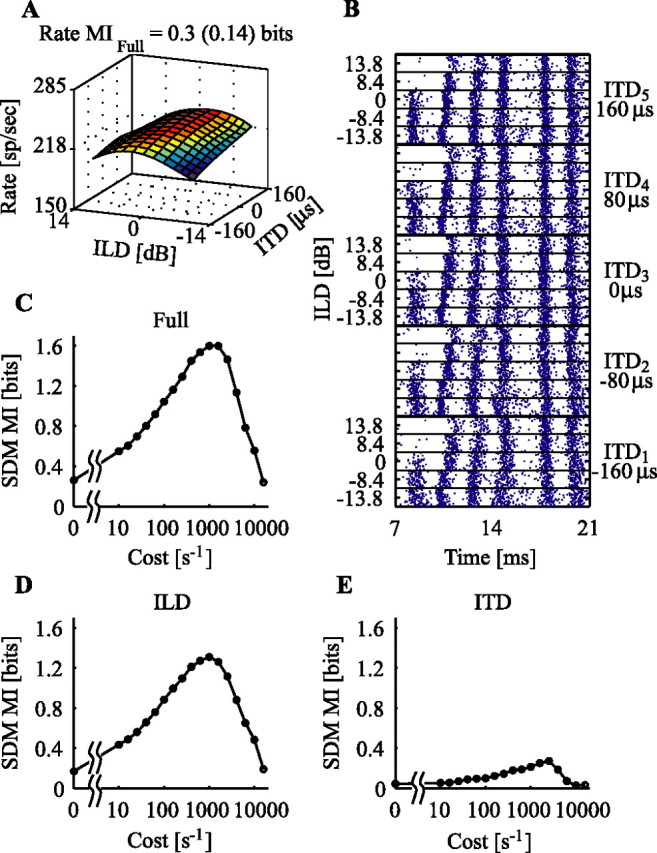
Responses of one neuron to the ITD/ILD stimulus set. A, Surface plot of the mean spike rate as a function of ITD and ILD. The rMI is shown above the plot, with the bias value in parentheses. (The surface was smoothed with cubic-spline interpolation.) B, Spike rasters to all 25 stimuli showing the first six spike bursts. Thick black lines divide different ITD parameters, shown at right; thin black lines divide different ILD parameters, shown at left. A total of 110 repetitions of each stimulus were collected. C, MI measured with the SDM method as a function of the spike-shift cost parameter for the full stimulus set. Note that 0 cost has been put at the 1 s⁻¹ position. D, MI_ild versus cost. E, MI_itd versus cost.

In the second stimulus set, average binaural intensity (ABI) (computed as the mean sound pressure level across the two ears) and ILD were manipulated. This set was designed to disambiguate monaural level responses from true binaural sensitivity. In this case, the frozen noise was again filtered through the spatially averaged HRTF. The result was attenuated to set an overall ABI (ranging from −8 to 8 dB in five equal steps) and then split into two streams that were attenuated relative to one another to impart an ILD that preserved that ABI.

In the third stimulus set, ILD and SN were varied. The SN cue was imparted by filtering the frozen-noise token through one of five midline HRTFs containing a prominent spectral notch, representing elevations ranging from 0 to 30° in 7.5° steps [Chase and Young (2005), their Fig. 2]. The stimulus was then split into two streams, and an ILD cue was imparted as in the ITD/ILD stimulus set. Interaural spectral differences were not considered in this work, because the same stimulus spectrum was sent to each ear. Before presentation, the stimuli in this set were resampled (resample command in Matlab; MathWorks, Natick, MA) such that the five SNs spanned the BF of the neuron under study with the notch frequency of the third stimulus at BF. Note that this resampling sometimes draws the SNs outside of the physiological range (6–20 kHz) (Musicant et al., 1990; Rice et al., 1992). The resampling also changes the stimulus length. Stimuli longer than 400 ms were truncated at 400 ms, whereas stimuli shorter than 200 ms were repeated to be at least 200 ms long.

The stimuli described above were all created from a single sample of noise, a frozen noise. In this case, the analysis is sensitive to phase locking to temporal stimulus features, which may be useful information for the auditory system but may or may not be a useful cue for sound localization. In a number of neurons, the SN/ILD stimulus set was modified to use a different noise on each stimulus presentation. In these cases, each repetition of the 25 SN/ILD stimuli was modified by adding a random vector, sampled from the uniform distribution over [(0,2π), to the stimulus phases in the Fourier domain. This has the effect of randomizing the temporal structure between sets of stimuli while holding the spectral magnitudes constant. For the analysis done here, these stimuli eliminated information in the stimulus envelope but preserved information in the spectral magnitudes. To minimize the effects of nonstationarity in the neural response, random-waveform sets were presented interleaved with the frozen set.

Spike distance metric.

The SDM developed by Victor and Purpura (1997) was used to assess the role of spike timing in conveying information. Essentially, the distance between two spike trains is defined as the sum of the costs of the elementary steps it takes to transform one spike train into the other. The allowed steps are spike deletion (cost of 1), spike addition (cost of 1), and spike shift (cost of q|Δt|), where Δt is the time difference between a spike in one train and the nearest spike in the other train, and q is a variable cost parameter (units of s⁻¹). For a given q, there exists a minimum cost solution for the distance between any two spike trains. A schematic of the distance calculation is presented in Figure 1A.

Figure 1.

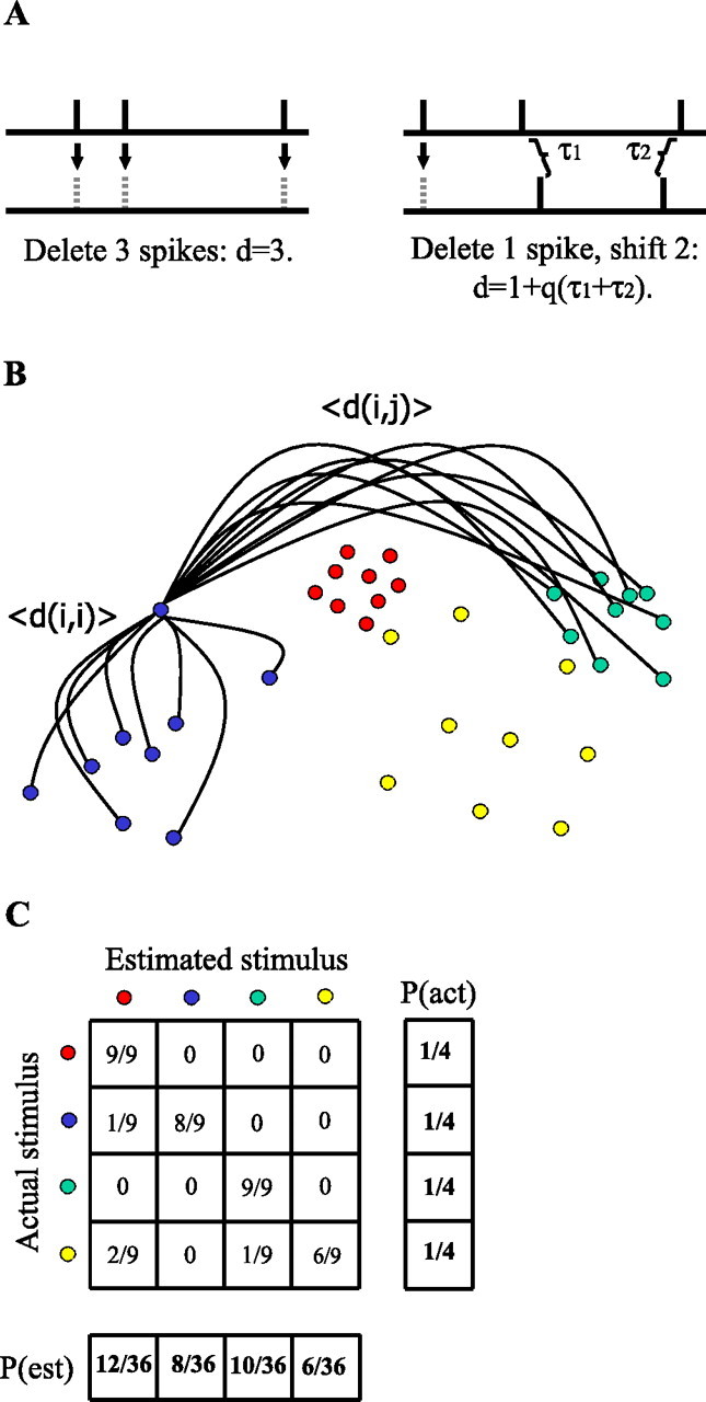
MI calculation using the spike distance metric. A, Spike distance calculation examples. Left, To turn the top spike train into the bottom spike train, three spikes must be deleted. Right, To turn the top spike train into the bottom spike train, one spike must be deleted and two spikes shifted. This is the minimum-cost solution for all cost parameters q such that qτ_i < 2 ∀ i. When this condition is not met, the spike is deleted from its position in the top train and added to the corresponding spot in the bottom train, adding a distance of 2. B, Stimulus clustering with the SDM method. Each dot represents a spike train whose color denotes the stimulus played when the train was recorded. For each train, the average distance 〈d(i,j)〉 to each group of spike trains is calculated. The spike train is estimated to have come from the stimulus group to which the average distance is smallest. C, A confusion matrix counts the number of spike trains assigned to each stimulus class. When normalized by the total number of spike trains, this is the joint stimulus response matrix used to calculate the MI.

The cost parameter q represents the precision with which spikes are timed. If q|Δt| > 2, it is cheaper to add and delete a spike than it is to shift it. Thus, 1/q is proportional to the time interval between spikes at which they are considered to be different, which can be interpreted as the integration time of a neuron reading the spike train. If q = 0, the only distance assigned between spike trains is the difference in their absolute number of spikes, which represents a rate code. At the other extreme, as q approaches infinity, the reading neuron performs a coincidence detector function in which spikes are not considered associated unless they occur at exactly the same time.

With the notion of spike-train distance defined, for any given spike train in response to stimulus i, it is possible to calculate the average distance to every other spike train measured from that neuron elicited by stimulus i, 〈d(i,i)〉. This average distance can then be compared with the average distance between the spike train and every spike train elicited by stimulus j, 〈d(i,j)〉. Figure 1B illustrates this idea, in which the dots represent spike trains and colors represent the stimuli being presented when the spike trains were measured. To a reading neuron, dots that cluster closest together should produce the most similar responses. To compute the information between stimuli and spike-train distances, the spike trains are assigned to the groups to which they are closest, regardless of the actual stimulus. That is, the spike train i is estimated to have come from stimulus j when j satisfies

After repeating this process for every spike train, a confusion matrix N is created where N(i,j) represents the number of times a spike train from stimulus i is classified as being closest to spike trains from stimulus j (Fig. 1C). The confusion matrix, when normalized by the total number of stimulus presentations, defines the joint stimulus/response probability on which MI (defined below) is calculated. As a stimulus estimation technique, the SDM allows the computation of a lower bound on the MI between stimuli and responses in a way analogous to other decoding techniques (Kjaer et al., 1994; Rolls et al., 1997; Furukawa and Middlebrooks, 2002).

Because the distance metric is a function of q, the MI calculated with this method is also a function of q. In addition to the q = 0 case, q was set to range from 10 to 15,850 s⁻¹ (100–0.063 ms), sampled logarithmically at 5 costs per decade. These costs were found empirically to cover the relevant range of timing resolutions of the ICC neurons studied.

Spike trains beginning at stimulus onset and extending 20 ms past stimulus offset were used in this analysis. However, when comparing MI results across neurons with different BFs, the analysis window was truncated at 200 ms to eliminate differences in stimulus length.

Mutual information.

Responses were analyzed by computing the MI between stimulus and response. The response was defined either as the discharge rate or as the result of the SDM calculation. The stimulus could either be the full 25 stimulus set containing variation of two stimulus parameters or a reduced set in which the variation of one stimulus parameter was ignored so that a five stimulus set was defined by combining the stimuli across the other parameter.

The MI between the response of a neuron, R, and the stimulus, S, is defined as follows (Cover and Thomas, 1991):

When the response is discharge rate, the MI is computed directly from empirical distributions of spike counts; that is, p(s,r) is the probability of getting a certain spike count r for a stimulus s. This method, including the debiasing methods, has been fully explained previously (Chase and Young, 2005).

For the SDM method, MI was calculated from the confusion matrix described above, in which s is the actual stimulus presented and r is the estimated stimulus from the cluster analysis. The probabilities were calculated from the counts in the confusion matrix, such that p(s,r) is the ratio of the counts in a particular bin to the total count summed over the whole matrix, and p(s) and p(r) are the ratios of the marginal counts to the total count. The MI for the full stimulus set (25 stimuli) was computed from the full confusion matrix. The MIs for the two independently varying cues were computed by combining the rows in the confusion matrix having the same value of the parameter of interest.

For notational convenience, the information between the response and the full stimulus set, MI(S;R), will be referred to as MI_full, and the information between the response and an individual localization cue (X or Y) will be referred to as MI_X or MI_Y. Mutual information calculated from discharge rate is called rMI. The full information can be broken down into the contributions from each localization cue as follows:

A derivation of this equation is provided by Chase and Young (2005). Essentially, this equation emphasizes that the MI between the response and the full stimulus set is always greater than or equal to the sum of the MIs about each of the individual cues, because the last term cannot be negative. MI(X;Y|R) is also known as the confounded information (Reich et al., 2001) and is related to the (lack of) independence in the neural response. For example, when the spike count in response to parameter X depends on the value of parameter Y, the confounded information in the spike-rate code will be non-zero. More importantly, non-zero confounded information means that the cues cannot be decoded independently.

For this study, the maximum value of MI_full is determined by the number of stimuli in the set. Because each of the stimulus sets in this study consists of 25 stimuli presented with equal probability, MI_full ≤ log₂(25) ≅ 4.6 bits. Similarly, MI_X is bound from above by log₂(5) ≅ 2.3 bits.

Estimates of MI based on finite datasets are subject to bias (Treves and Panzeri, 1995; Panzeri and Treves 1996; Paninski, 2003). For both the rate and SDM methods, MI estimates were bias corrected with a bootstrap procedure (Efron and Tibshirani, 1998). In the rate case, 500 bootstrap datasets for each stimulus were derived by randomly drawing (with replacement) M spike counts from the recorded set of spike counts for that stimulus, where M is the number of stimulus repetitions. For the SDM case, 500 bootstrap confusion matrices were generated by randomly drawing (with replacement) from the counts of the confusion matrix. That is, each row of the bootstrapped confusion matrix was generated by selecting counts from the corresponding row of the original matrix, keeping the total count in each row fixed. In simulations, this procedure was found to converge to the true MI value faster than other debiasing methods, such as randomly reassigning stimuli and responses (data not shown). Data from neurons for which fewer than 20 repetitions of each stimulus were gathered were not included in this analysis. Because of the high number of stimulus repetitions typically achieved (median of 70 repetitions), the estimated bias for MI_full was quite low (rate, median of 0.11 bits; SDM peak, median of 0.08 bits). All values of MI presented in this paper are bias corrected.

Results

Figure 2 shows an example of a neuron studied with the ITD/ILD stimulus set presented at a high sound level. As often happens at high levels, the rate response is saturated (Fig. 2A), so the rate information about the full stimulus set (rMI_full) is only 0.3 bits. Although there is little consistent change in the spike count among stimuli, a close-up view of the spike rasters (Fig. 2B) shows considerable variation in individual spike times with ILD. In particular, whereas the first burst is either on or off depending on the ILD, the second, third, and fourth bursts are progressively delayed with increases in ILD. Figure 2C shows the results of the SDM analysis on these spike trains. For a spike-shift cost of 1000 s⁻¹, 1.6 bits of information is recovered about the stimulus identity. This maximum is called MI_peak, and the cost at which it occurs is called the peak cost. The cost = 0 case, which represents a rate code, is called MI₀. Finally, the largest cost at which the MI decays to half of its peak value is known as the cutoff cost, which is ∼4000 s⁻¹ for the neuron in Figure 2C. The MIs to the individual location cues are shown in Figure 2, D and E. As expected from the raster plot, most of the information in MI_full is about ILD.

Figure 3 shows another example; in this case, there is little extra information available in spike timing that is not available in rate. The rate surface of Figure 3A shows considerable variation in response to both stimulus parameters, and indeed rMI_full is quite high at 2.3 bits. The MI(cost) curve from the SDM analysis shows a nearly low-pass behavior (Fig. 3C), with only a small peak that would indicate extra information available in spike timing. Note that this is not because this neuron does not exhibit stimulus locking, as shown in the raster plot (Fig. 3B). Rather, the variation in spike timing across stimuli is not significant compared with the rate differences.

Figure 3.

Another example of information extraction with the SDM method. The format is as in Figure 2, with the exception that the three MI(cost) curves have been condensed to a single plot.

The results in Figures 2 and 3 exemplify the range of behavior shown by the population; typically, responses lie between these two extremes. The information carried in spike patterns about the full stimulus set, as assessed with the SDM method, is shown as a function of BF in Figure 4A for all neurons in this study. To assess possible differences across groups, we used an ANOVA calculation with a significance criterion of p = 0.05 corrected for multiple comparisons. Frequency was divided into three equally populated groups (low, middle, and high) to assess the effects of BF as an independent variable. There are no differences in the MI_peak values across the three stimulus sets, so they are not differentiated in this plot. There are also no differences in MI_peak across the neuron types or in differences in MI_peak values with BF.

Figure 4.

SDM information carried about the full stimulus set. V, I, and O symbols correspond to the physiological neuron type. A, MI_peak plotted as a function of BF for all neurons and stimuli. B, MI_peak as a function of the information calculated directly from the spike rates. C, MI from the SDM method at 0 cost plotted as a function of the MI calculated directly from discharge rate.

To view the amount of information available in temporal spike patterns that is not available in spike rate, MI_peak from the SDM calculation is plotted as a function of the information calculated assuming a rate code in Figure 4B. The vertical offset of the points from the diagonal represents the extra information available when spike timing is taken into account. Many neurons show a considerable information gain with the SDM method.

Recall that, for the 0 cost (q = 0) analysis, no penalty is assigned to shifting spikes, only to adding or deleting them. This case should, then, correspond to a rate code, and the information calculated from the SDM method at 0 cost should be the same as the information calculated under the assumption of a rate code, if no information is lost in the decoding step when the confusion matrix is generated. When MI₀ is plotted as a function of rMI for each neuron, there is very good agreement between the two measurements (r = 0.99) (Fig. 4C).

In Figure 5, MI_peak values are compared with the corresponding rMI measures for each of the individual localization cues. For ITD information (Fig. 5A), the points all cluster along the diagonal, showing that very little extra information is available when considering spike timing. This strongly suggests that, at the level of the ICC, ITD information is carried in a rate code. The coding of ILD cues is shown in Figure 5B, in which ILD cues from all three stimulus sets have been lumped together because the populations overlap. The SDM method recovers a mild amount of information about ILD cues over that available through a rate code. The same holds true for ABI cues (Fig. 5C), which show less information, on average, than the other cues. The largest effect of spike timing is on the coding of SN cues (Fig. 5D). In general, the MI in SDM responses to SN is much larger than the MI in rate responses to SN. For some neurons, as much as 2 bits of information is recovered by considering spike timing.

Figure 5.

Comparison between the peak information calculated with the SDM method and rMI for individual localization cues. A, ITD. B, ILD. C, ABI. D, SN. E, Spike-timing gain (MI_peak − MI₀) as a function of BF for the SN cue.

The spike-timing gain for SN information is plotted as a function of BF in Figure 5E. This gain is defined as the difference between MI_peak and MI₀ and represents information only available through spike timing. The spike-timing gain is negatively correlated with BF (r = −0.48; df = 56; p < 0.0001); it is mainly the low-BF neurons that carry the extra information about SN in the timing of spikes, although there are some midfrequency neurons with spike-timing gains of as much as 1 bit. The largest spike-timing gains are seen in type V neurons, which are found only at low BFs (Ramachandran et al., 1999) and are the predominant low-BF response type in our sample. This point is discussed in more detail in Discussion.

Timescale of information

The cost at which MI is maximum is a measure of the temporal precision of the spike patterns that provide information captured by the SDM analysis. As discussed in Materials and Methods, 1/q is a measure of the effective integration time of a neuron reading the temporal information in spike patterns, in the sense that 2/q is the maximum time delay between spikes in two trains at which they can still be shifted into alignment.

Figure 6 shows data on the costs at which the maximum MI is obtained with the SDM analysis, for each of the localization cues studied. The median peak cost value obtained by pooling cost values from all localization cues and ignoring 0 values is ∼80 s⁻¹. Thus, when there is localization information in spike timing, it is integrated on a timescale of ∼12 ms.

Figure 6.

Timescale of the temporal representation of localization cues. A, Cost at which the SDM MI reached its peak value plotted as a function of BF for the ITD cue. Note that the 0 cost data points have been placed at the 1 s⁻¹ spot. B, ILD. C, ABI. D, SN. The black line represents the best linear fit of log(cost) to log(BF), ignoring 0 cost values.

A peak cost of 0 was declared if the MI_peak value remained within 10% of MI₀ for that neuron (for example, the ILD curve in Fig. 3C), indicating that most of the information was carried by rate. Peak costs of 0 occurred in 50% of the ITD cases (Fig. 6A) and 41% of the ILD cases (Fig. 6B). This is in comparison with only 12% of cases for the ABI cue (Fig. 6C) and 9% of cases for the SN cue (Fig. 6D).

The other major difference between the information timescales for different localization cues is that there is a significant correlation between BF and peak cost for the SN cue (r = −0.46; df = 48; p = 0.0004, ignoring 0 cost values) that is not seen with the other cues. SNs are represented at finer timescales in low-BF neurons than they are in high-BF neurons.

Frozen versus random noise

In this section, we show that the information that is recovered by the SDM analysis is almost entirely derived from locking to temporal features of the stimulus. To demonstrate this point, responses to frozen noise, for which the temporal waveform is the same in all stimulus repetitions, were compared with responses to phase-randomized noise, for which the temporal waveform differs in each repetition. Information that depends on the temporally locked stimulus features will not be present with the random noise. All data presented to this point were obtained with frozen noise.

Figure 7 shows the responses of a 1.8 kHz type O neuron in response to the random/frozen stimulus set described in Materials and Methods. There is very little difference in the average rate responses, as shown in Figure 7, A and B, and the rMI_full of these stimulus sets are nearly identical at ∼0.65 bits. The temporal responses to the two stimulus sets are completely different, however, as shown by the raster plots in Figure 7, C and D. From the raster to the frozen noise, it is clear that this neuron responded to specific temporal events in the stimuli, events that occur at fixed times in the frozen noise but not in the random noise. As an example, there is a spike that occurs frequently at a latency of ∼56 ms in the responses to two of the frozen SN stimuli (1.8 and 1.7 kHz) but not in the others. The only apparent temporal feature that remains in the random noise is the latency of the first burst of spikes, which changes systematically with ILD in both stimulus sets.

Figure 7.

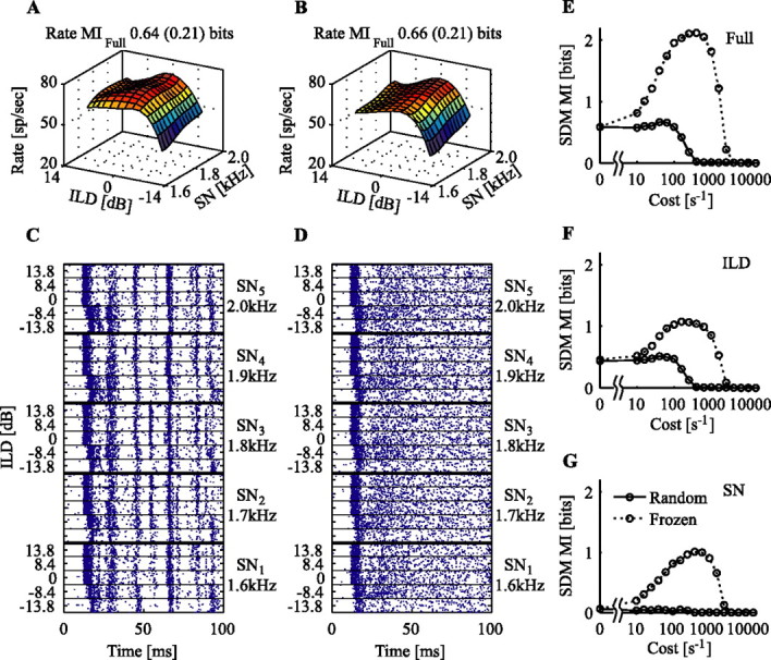
Responses of a 1.8 kHz neuron to the frozen- and random-noise stimulus sets. A, Average firing rate as a function of SN and ILD for the frozen-noise stimulus set. Plotting conventions are as in Figure 2. B, Same, for the random-noise set. C, Spike rasters of the responses to the frozen-noise stimulus set. D, Rasters of the responses to the random-noise set. Note that the ILD-dependent latency differences remain, whereas most other time-locked responses vanish. E, SDM MI_full as a function of cost for the frozen (dotted) and random (solid) stimulus sets. F, SDM MI_ild(cost). G, SDM MI_sn(cost).

The SDM information carried by this neuron is shown in Figure 7E–G for both stimulus sets. As is characteristic of low-frequency neurons, there is a large peak in the MI(cost) curves for the frozen-noise set, indicating the presence of a substantial amount of information in spike timing over that in rate. These peaks are missing from the random-waveform responses. Thus, the extra information available in spike timing was attributable to the differences in the temporal waveforms within the frozen-noise SN/ILD stimulus set as opposed to an intrinsic variation in spike patterns stemming purely from spectral or level differences.

ILD-related latency differences were observed in both the responses to frozen and random waveforms (Fig. 7C,D). However, the SDM method reveals timing information in only the frozen-waveform case. This indicates that the SDM method, as computed here, is relatively insensitive to first-spike-latency variation. Although differences in spike latency must increase the distance between spike trains, this distance is apparently overwhelmed by other noisy sources of spike-train differences. When the SDM MI is computed using spike trains with all but the first spike removed (a first-spike latency code), 1.3 and 0.9 bits of information are recovered about the full stimulus set for the frozen- and random-waveform sets, respectively.

The results of the example neuron in Figure 7 are consistent across the population of neurons for which the random-waveform stimulus data were gathered. For the 13 neurons studied with the random-noise stimuli, the mean and SD of the spike timing gains for frozen noise were 0.54 ± 0.61 bits (range of 0–1.7 bits), whereas the corresponding spike-timing gain values for random noise were significantly less at 0.1 ± 0.06 bits (range of 0–0.25 bits; different from frozen noise at p < 0.01, signed rank test). ILD random-noise spike-timing gains were not significantly different from SN gains.

Relative information

The percentage of MI_full that is devoted to the coding of an individual localization cue is called the relative information. It is computed as the ratio MI_X/MI_full and is the basis for analyzing the interactions of individual localization cues. An example of this computation is given in Figure 8 for a type V neuron in response to the SN/ILD stimulus set (with frozen noise). Figure 8A shows MI_full, MI_ild, and MI_sn as a function of cost. At ∼630 s⁻¹, this neuron shows a prominent peak of 3.5 bits in its MI_full(cost) curve (one of the most sensitive neurons in the population), a gain of ∼2 bits over its 0 cost value. Although it is clear from Figure 8A that MI_ild and MI_sn covary with MI_full, Figure 8B shows that the fraction of MI_full devoted to ILD or SN coding is not constant with cost. Instead, there is a monotonic increase in the MI_sn percentage as a function of cost, whereas MI_ild shows a low-pass behavior.

Figure 8.

An example cost/coding trajectory. A, MI(cost) curves for an example neuron in response to the SN/ILD stimulus set. B, Relative information [MI (as percentage)] plotted as a function of cost. Here, MI_sn and MI_ild are normalized by MI_full and plotted as percentages. Their sum is plotted as a dotted line. C, The percentage of information devoted to SN coding is plotted as a function of that devoted to ILD coding for each cost studied; certain trajectory points are labeled with their cost values (units of s⁻¹). The arrow represents the summary trajectory from 0 cost to the cutoff cost (6310 s⁻¹ for this neuron).

This result is further summarized in Figure 8C. Here, the “trajectory” of single-cue coding is plotted. Each dot plots the relative information for SN versus ILD at a particular cost. Points lie below the diagonal when MI_full is not equal to the sum of the information in the individual cues or when the confounded information of Equation 3 is non-zero. At a cost of 0 (rate case), the confounded information is large; MI_sn and MI_ild are not independently represented in the neural response. As the cost parameter is increased, the confounded information decreases until it reaches 0 (near 50 s⁻¹), signifying that SN and ILD are independently coded. Finally, at costs over 1000 s⁻¹, the information about both ILD and SN (and MI_full) decreases. The decrease is faster for ILD, so the points in Figure 8C move toward the upper left-hand corner of the plot.

The reduction in confounded information with increasing cost is a general trend across the population. Considering only those neurons sensitive to both cues in the stimulus set (defined as having a relative rMI_X ≥ 10% for each cue; n = 94), the median confounded information at 0 cost is 24%, whereas the median confounded information at peak cost is 15% (the two are different at p < 0.00001, rank sum test). Because rate is a unidimensional measure, using a rate code to represent more than one cue necessarily leads to a confounded representation of the encoded quantities. The extra dimensions of spike timing allow a more independent representation of the localization cues and, in theory, allow the cues to be decoded more independently, as well.

SN/ILD coding trajectories for the entire population are summarized in Figure 9. This plot shows vectors, such as the arrow in Figure 8C, that point from the 0 cost position in the relative information plot to the cutoff cost position (in which the SDM MI has decayed to half of its peak value). The arrows are translated so the 0 cost position is at the origin; thus, the lines represent the changes in relative information as cost increases. Only neurons for which both individual cue MI_peak values are >0.2 bits are considered. The gray lines represent the change in relative information from 0 cost to cutoff cost for individual neurons, and the mean trajectory for the whole population is given as the thick black line. Trajectories pointing to negative values on the abscissa represent cases in which the percentage of MI_full devoted to coding ILD decreases over its 0 cost value when spike timing is taken into account; trajectories pointing upward represent cases in which the percentage devoted to SN increases with cost.

Figure 9.

Cost coding summary trajectories for the population in response to the SN/ILD stimulus set. Individual coding trajectories are shown in gray, and the population mean is shown in black. The inset shows a close-up view of the population mean. Red dots represent population means resulting from bootstrap resampling of the individual trajectories; 1000 bootstrap samples were used.

There is remarkable consistency in the coding trajectories across the population, with the majority of trajectories heading in approximately the same direction. As the absolute timing of spikes becomes relevant in the code, the representation of SN increases, and the representation of ILD decreases. To test the significance of this result, the calculation of the population means was repeated 1000 times with bootstrap sampling from the trajectory vectors. The results are shown in the inset, in which the red dots correspond to the endpoints of the mean trajectory vectors from the bootstrapped datasets. Essentially, the cloud of red dots represents the two-dimensional confidence interval of the mean trajectory vector endpoint. All of the bootstrapped values lie in the second quadrant, indicating that the change in coding representation from ILD to SN with increasing temporal resolution is a general, significant trend of the population.

For the ITD/ILD and ABI/ILD sets, the general behavior is similar. However, the vectors are shorter because of the relatively small amount of MI revealed by the SDM analysis for ITD and ABI. The trend with the ITD/ILD set is for MI_ild/MI_full to increase at the expense of MI_itd/MI_full, and, for the ABI/ILD set, MI_abi/MI_full increased at the expense of MI_ild/MI_full (data not shown).

Discussion

Temporal representation of sound localization cues in ICC

The question asked here is whether the temporal patterns of spike trains can enhance the representation of sound localization cues in the ICC. Conceptually, such temporal information could be stimulus locked (e.g., by phase locking to the waveform of the stimulus), or not stimulus locked. In the latter case, sound localization cues would be represented by changes in the temporal patterns of spiking that are not directly related to the temporal waveform of the stimulus, as in the work in visual cortex by Optican and Richmond (Optican and Richmond, 1987; Richmond and Optican, 1990). Of course, most auditory neurons, including those in the ICC, lock strongly to the stimulus envelope (Joris, 2003; Louage et al., 2003). Thus, evaluation of nonstimulus-locked temporal coding must control for these envelope responses; here we used random noise, for which envelope locking should not provide consistent information from one stimulus to the next.

We use an SDM analysis to look at temporal coding. An important check on this analysis is the fact that the 0 cost MI is the same as the discharge rate MI (rMI ≈ MI₀ in Fig. 4C). Because the SDM method is based on stimulus parameter estimation, it provides a lower bound to the information available in the spike trains. For the 0 cost case, the SDM method recovers all of the information available; however, this is not true at higher costs, because we know the method is insensitive to first-spike-latency information (discussed below). Thus, the information increment analysis (Fig. 5) should be looked on as a lower bound to the extra temporal information that is available in spike trains.

The results show that encoding in spike timing potentially enhances the amount of information carried about localization cues in ICC (Figs. 4, 5). Significant timing-dependent increments were seen for all of the cues except ITD, with the largest effects for SN. The lack of ITD-related temporal information suggests that ITD is represented by discharge rate alone in ICC. This is consistent with the work of Carney and Yin (1989), who investigated the effects of ITD manipulation in a population of low-frequency ICC neurons. Their raster plots of neurons responding to broadband noise at various ITDs (compare with their Figs. 10, 11) show that there is little change in the timing of spikes to changes in ITD; rather, there is a large ITD-dependent gain change.

The position of the peak in MI versus cost functions (Fig. 2C–E) provides an estimate of the timescale at which spike timing provides the most information. The data of Figure 6 show that localization cues in the ICC are best decoded at a cost of ∼80 s⁻¹, suggesting that the resolution of localization-related spike-timing patterns in the ICC is ∼12 ms.

The nature of the temporal representation

When random noise was used to eliminate stimulus-waveform cues, the only temporal information remaining in IC neurons was that encoded in first-spike latency. Sound location has been shown to modulate the first-spike latency in both IC and auditory cortex (Brugge et al., 1996; Furukawa and Middlebrooks, 2002; Sterbing et al., 2003; Mrsic-Flogel et al., 2005). Although latency differences contribute to the distances measured with the SDM, in practice, the variation in spike-train distances caused by latency are too small to have much effect on stimulus grouping, unless the analysis is confined to the first few spikes. The analysis of temporal information presented here does not address the role that first-spike latency may play in encoding sound-localization cues.

The frozen/random-noise analysis (Fig. 7) shows that the temporal patterns are mainly locked to temporal features of the stimulus waveform, independent of static localization cue values. The largest stimulus-waveform effects are related to SN cues. Presumably, these represent phase locking to the temporal envelope of the stimulus induced by the sharp antiresonances in the SN stimuli. The strongest temporal information about SN occurs at BFs below the physiological range of SN cues in cats (Musicant et al., 1990; Rice et al., 1992). This suggests that the temporal increments for SN stimuli do not represent a specialization for representing SN. Instead, the temporal information is induced by spectral irregularities or temporal envelopes in general, as for example in speech (Bandyopadhyay and Young, 2004).

Can the temporal information identified here be used by the auditory system for sound localization? To do so, there would have to be a template for the spike trains expected from a known stimulus (i.e., the stimulus would have to be recognized by the auditory system on the basis of its other properties). Then its location could be determined in part through the envelope induced by SN cues as demonstrated here. However, this source of information would be vulnerable to echoes and other environmental phase distortions, limiting its usefulness as an absolute localization cue.

A situation in which temporal cues might contribute is when comparisons of two stimuli occurring in the same acoustic environment are possible (e.g., in determining when a given sound source has changed location). In binaural-masking-level-difference experiments, random noises are more effective at masking interaural correlation differences than frozen noises (Breebaart and Kohlrausch, 2001) because of the uncertainty in the interaural correlation of the masker. This result suggests that minimum audible angles for random-noise stimuli should be higher than for frozen stimuli, because of better encoding of SN cues in the latter case. Another situation in which temporal locking would be useful would be in the comparison of spike times across different neurons. This type of population encoding is not considered in this analysis.

Perhaps more surprising than the temporally locked SN information is the temporally locked ILD information. ILD is a static cue, yet its representation in the neural response benefits from spike times locked to the stimulus. When the ILD is changed, events in the stimulus that were subthreshold could become superthreshold and cause the neuron to spike. These spikes would force the neuron into its refractory period and may affect the position of the next burst of spikes. Thus, changes in ILD could cause a rearrangement in the peristimulus time histogram (PSTH). Of course, the same argument could be made for changes in ITD, which do not result in rearrangements in the PSTH; the mechanisms behind ILD and ITD encoding need to be further explored.

Differences among ICC neuron classes

In a previous publication (Chase and Young, 2005), the information about localization cues provided by ICC neurons of three different response types was compared. That analysis, based only on discharge rate, found that, although there were some differences among the neuron types, generally there was substantial overlap in the information provided by the three classes of neurons. The largest differences were for the type V neurons, which provided information mainly about ITD and ABI. Type V neurons stand out in the present analysis by showing larger MI increments than the other neuron types when spike timing is considered. Because type V neurons are found only at low BFs and because most of the neurons in the low-BF sample were type V, it is not clear whether the difference has to do with BF or with the particular circuitry connected to the type V neurons. An argument for the former is that the changes in temporal envelope produced by shifting the location of a spectral notch will be at higher envelope frequencies for high-BF neurons compared with low-BF neurons. Given that neurons in the ICC have a cutoff frequency in their modulation transfer functions of ∼100 Hz (Langner and Schreiner, 1988; Krishna and Semple, 2000), it may be that the temporally coded information produced by changes in SN frequency is outside the modulation response regions of neurons or high-BF neurons.

The representation of multiple cues

These results show that spike-timing codes can reduce the confounded information in the response, allowing individual cues to be represented more independently (Figs. 8, 9). Furthermore, the representation of cues in the response changes as a function of the decoding time resolution in a consistent manner, as illustrated for SN/ILD stimuli by Figure 9. ITDs are coded on the longest timescales, by spike rate. ILDs are coded at intermediate timescales because increases in the SDM cost cause an increase in ILD information relative to ITD information but a decrease relative to SN information. SN information is available at the shortest timescales, especially in low-frequency neurons. Together, these results imply that spike timing could play an important role in multiplexing information onto spike trains, given appropriate decoding mechanisms.

References

- Adams JC (1979). Ascending projections to the inferior colliculus. J Comp Neurol 183:519–538. [DOI] [PubMed] [Google Scholar]
- Bandyopadhyay S, Young ED (2004). Discrimination of voiced stop consonants based on auditory nerve discharges. J Neurosci 24:531–541. [DOI] [PMC free article] [PubMed] [Google Scholar]
- Benevento LA, Coleman PD (1970). Responses of single cells in cat inferior colliculus to binaural click stimuli: combinations of intensity levels, time differences, and intensity differences. Brain Res 17:387–405. [DOI] [PubMed] [Google Scholar]
- Breebaart J, Kohlrausch A (2001). The influence of interaural stimulus uncertainty on binaural signal detection. J Acoust Soc Am 109:331–345. [DOI] [PubMed] [Google Scholar]
- Brugge JF, Reale RA, Hind JE (1996). The structure of spatial receptive fields of neurons in primary auditory cortex of the cat. J Neurosci 16:4420–4437. [DOI] [PMC free article] [PubMed] [Google Scholar]
- Brunso-Bechtold JK, Thompson GC, Masterton RB (1981). HRP study of the organization of auditory afferents ascending to central nucleus of inferior colliculus in cat. J Comp Neurol 197:705–722. [DOI] [PubMed] [Google Scholar]
- Caird D, Klinke R (1987). Processing of interaural time and intensity differences in the cat inferior colliculus. Exp Brain Res 68:379–392. [DOI] [PubMed] [Google Scholar]
- Carney LH, Yin TCT (1989). Responses of low-frequency cells in the inferior colliculus to interaural time differences of clicks: excitatory and inhibitory components. J Neurophysiol 62:144–161. [DOI] [PubMed] [Google Scholar]
- Chase SM, Young ED (2005). Limited segregation of different types of sound localization information among classes of units in the inferior colliculus. J Neurosci 25:7575–7585. [DOI] [PMC free article] [PubMed] [Google Scholar]
- Cover TM, Thomas JA (1991). In: Elements of information theory New York: Wiley.
- Delgutte B, Joris PX, Litovski RY, Yin TCT (1995). Relative importance of different acoustic cues to the directional sensitivity of inferior-colliculus neurons. In: Advances in hearing research (Manley GA, Klump GM, Köppl C, Fastl H, Oeckinghaus H, eds) pp. 288–299. River Edge, NJ: World Scientific.
- Delgutte B, Joris PX, Litovski RY, Yin TCT (1999). Receptive fields and binaural interactions for virtual-space stimuli in the cat inferior colliculus. J Neurophysiol 81:2833–2851. [DOI] [PubMed] [Google Scholar]
- Efron B, Tibshirani RJ (1998). In: Introduction to the bootstrap Boca Raton, FL: CRC.
- Furukawa S, Middlebrooks JC (2002). Cortical representation of auditory space: information-bearing features of spike patterns. J Neurophysiol 87:1749–1762. [DOI] [PubMed] [Google Scholar]
- Joris PX (2003). Interaural time sensitivity dominated by cochlea-induced envelope patterns. J Neurosci 23:6345–6350. [DOI] [PMC free article] [PubMed] [Google Scholar]
- Kjaer TW, Hertz JA, Richmond BJ (1994). Decoding cortical neuronal signals: network models, information estimation and spatial tuning. J Comput Neurosci 1:109–139. [DOI] [PubMed] [Google Scholar]
- Krishna BS, Semple MN (2000). Auditory temporal processing: responses to sinusoidally amplitude-modulated tones in the inferior colliculus. J Neurophysiol 84:255–273. [DOI] [PubMed] [Google Scholar]
- Kuhn GF (1977). Model for the interaural time differences in the azimuthal plane. J Acoust Soc Am 62:157–167. [Google Scholar]
- Langner G, Schreiner CE (1988). Periodicity coding in the inferior colliculus of the cat. I. Neuronal mechanisms. J Neurophysiol 60:1799–1822. [DOI] [PubMed] [Google Scholar]
- Louage DHG, van der Heijden M, Joris PX (2003). Temporal properties of responses to broadband noise in the auditory nerve. J Neurophysiol 91:2051–2065. [DOI] [PubMed] [Google Scholar]
- Middlebrooks JC, Clock AE, Xu L, Green DM (1994). A panoramic code for sound location by cortical neurons. Science 264:842–844. [DOI] [PubMed] [Google Scholar]
- Mrsic-Flogel TD, King AJ, Schnupp JWH (2005). Encoding of virtual acoustic space stimuli by neurons in ferret primary auditory cortex. J Neurophysiol 93:3489–3503. [DOI] [PubMed] [Google Scholar]
- Musicant AD, Chan JCK, Hind JE (1990). Direction-dependent spectral properties of cat external ear: new data and cross-species comparisons. J Acoust Soc Am 30:237–246. [DOI] [PubMed] [Google Scholar]
- Nelken I, Chechik G, Mrsic-Flogel TD, King AJ, Schnupp JWH (2005). Encoding stimulus information by spike numbers and mean response time in primary auditory cortex. J Comp Neurosci 19:199–221. [DOI] [PubMed] [Google Scholar]
- Oliver DL, Beckius GE, Bishop DC, Kuwada S (1997). Simultaneous anterograde labeling of axonal layers from lateral superior olive and dorsal cochlear nucleus in the inferior colliculus of cat. J Comp Neurol 382:215–229. [DOI] [PubMed] [Google Scholar]
- Optican LM, Richmond BJ (1987). Temporal encoding of two-dimensional patterns by single units in primate primary visual cortex. I. Information theoretic analysis. J Neurophysiol 57:162–178. [DOI] [PubMed] [Google Scholar]
- Paninski L (2003). Estimation of entropy and mutual information. Neural Comput 15:1191–1253. [Google Scholar]
- Panzeri S, Treves A (1996). Analytical estimates of limited sampling biases in different information measures. Netw Comput Neural Syst 7:87–107. [DOI] [PubMed] [Google Scholar]
- Ramachandran R, Davis KA, May BJ (1999). Single-unit responses in the inferior colliculus of decerebrate cats. I. Classification based on frequency response maps. J Neurophysiol 82:152–163. [DOI] [PubMed] [Google Scholar]
- Reich DS, Mechler F, Victor JD (2001). Formal and attribute-specific information in primary visual cortex. J Neurophysiol 85:305–318. [DOI] [PubMed] [Google Scholar]
- Richmond BJ, Optican LM (1990). Temporal encoding of two-dimensional patterns by single units in primate primary visual cortex. II. Information transmission. J Neurophysiol 64:370–380. [DOI] [PubMed] [Google Scholar]
- Rice JJ, May BJ, Spirou GA, Young ED (1992). Pinna-based spectral cues for sound localization in cat. Hear Res 58:132–152. [DOI] [PubMed] [Google Scholar]
- Rieke F, Yamada W, Moortgat K, Lewis ER, Bialek W (1992). Real time coding of complex sounds in the auditory nerve. Adv Biosci 83:315–322. [Google Scholar]
- Rolls ET, Treves A, Tovee MJ (1997). The representational capacity of the distributed encoding of information provided by populations of neurons in primate temporal visual cortex. Exp Brain Res 114:149–162. [DOI] [PubMed] [Google Scholar]
- Roth GL, Aitkin LM, Andersen RA, Merzenich MM (1978). Some features of the spatial organization of the central nucleus of the inferior colliculus of the cat. J Comp Neurol 182:661–680. [DOI] [PubMed] [Google Scholar]
- Roth GL, Kochar RK, Hind JE (1980). Interaural time differences: implications regarding the neurophysiology of sound localization. J Acoust Soc Am 68:1643–1651. [DOI] [PubMed] [Google Scholar]
- Sterbing SJ, Hartung K, Hoffmann K (2003). Spatial tuning to virtual sounds in the inferior colliculus of the guinea pig. J Neurophysiol 90:2648–2659. [DOI] [PubMed] [Google Scholar]
- Treves A, Panzeri S (1995). The upward bias in measures of information derived from limited data samples. Neural Comput 7:399–407. [Google Scholar]
- Victor JD, Purpura KP (1997). Metric-space analysis of spike trains: theory, algorithms and application. Netw Comput Neural Syst 8:127–164. [Google Scholar]