Learning to See the Difference Specifically Alters the Most Informative V4 Neurons

Abstract

Perceptual learning is an instance of adult plasticity whereby training in a sensory (e.g., a visual task) results in neuronal changes leading to an improved ability to perform the task. Yet studies in primary visual cortex have found that changes in neuronal response properties were relatively modest. The present study examines the effects of training in an orientation discrimination task on the response properties of V4 neurons in awake rhesus monkeys. Results indicate that the changes induced in V4 are indeed larger than those in V1. Nonspecific effects of training included a decrease in response variance, and an increase in overall orientation selectivity in V4. The orientation-specific changes involved a local steepening in the orientation tuning curve around the trained orientation that selectively improved orientation discriminability at the trained orientation. Moreover, these changes were largely confined to the population of neurons whose orientation tuning was optimal for signaling small differences in orientation at the trained orientation. Finally, the modifications were restricted to the part of the tuning curve close to the trained orientation. Thus, we conclude that it is the most informative V4 neurons, those most directly involved in the discrimination, that are specifically modified by perceptual learning.

Introduction

Improvement in sensory discrimination after practice is a well documented behavioral phenomenon (Karni and Bertini, 1997; Goldstone, 1998; Gilbert et al., 2001; Fahle and Poggio, 2002; Ahissar and Hochstein, 2004), referred to as perceptual learning. Typically, learning-induced improvements in the discrimination of simple visual features display a high degree of stimulus specificity (Ramachandran and Braddick, 1973; Fiorentini and Berardi, 1981; Vogels and Orban, 1985), which has been used to infer the cortical locus at which such changes take place. Poor transfer of training effects to untrained orientations or locations has led previous authors investigating training-induced modifications of neuronal responses (Crist et al., 2001; Schoups et al., 2001; Ghose et al., 2002; Li et al., 2004) to focus on primary visual cortex, which contains a high proportion of orientation-specific neurons with small receptive fields.

Using orientation discrimination as a paradigm, Schoups et al. (2001) found an orientation- and location-specific increase in the slope of the orientation tuning curve of V1 neurons. These orientation- and position-specific tuning changes were restricted to the subpopulation of neurons with preferred orientations offset 20° from the trained orientation. Subsequent studies (Ghose et al., 2002; Yang and Maunsell, 2004) failed to find any changes in the orientation tuning of V1 or V2 neurons, but reported a narrowing of the orientation tuning curves in V4 neurons. This led to the suggestion that perceptual learning effects might be stronger in V4 than at earlier levels. Because the effects in V4 were most pronounced in neurons that preferred orientations close to the trained orientation, the results seemed to refute the view that training selectively alters the most informative neurons, those with steepest slope of their tuning curves at the trained orientation.

To resolve this discrepancy, we investigated the effects of learning an orientation discrimination on the neuronal properties of V4 neurons, duplicating the training and test procedures of the V1 study of Schoups et al. (2001). We not only compared the response properties for trained and control hemispheres but also determined whether there were any training effects specific to the trained orientation. More importantly, we investigated whether there might be training effects that targeted a specific subpopulation of V4 neurons, those with the steepest slope in tuning curve at the trained orientation. Finally, because fine discrimination involves only a small portion of the total bandwidth of the tuning curve (Paz et al., 2004), we also assessed whether any of the learning effects were restricted to the portion of the tuning curve corresponding to the trained orientation or affected the tuning curve as a whole. A mechanism that affects only a part of the tuning function will minimize the disturbance to visual representations that could potentially impair normal vision (Dosher and Lu, 1998; Ghose et al., 2002).

To maximize the chance of detecting orientation-specific changes we recorded from a large number of V4 neurons, fitted their responses to 16 orientations using a polynomial curve, and examined training effects at multiple points on the tuning curve, including the trained orientation.

Materials and Methods

Subjects.

Two adult male rhesus monkeys (monkeys 1 and 2) were trained in an orientation identification task. A third monkey (monkey 3) used as a control was trained only to fixate. Cells were recorded from two trained hemispheres in monkeys 1 and 2, and from two untrained, control hemispheres in monkeys 2 and 3, respectively. Subjects were equipped with polymer or stainless-steel headposts to fix the head to the primate chair during experiments. These implantations and all other surgical procedures were performed under general anesthesia (isoflurane/nitrous oxide) and sterile conditions. All animal care and experimental procedures met the national and European guidelines and were approved by the ethical committee of the Katholieke Universiteit Leuven Medical School. Monkey 1 was also provided with a scleral search coil to monitor eye position, but as our technique evolved, subsequent subjects were monitored using a noninvasive infrared eye-tracking device (Iscan, Burlington, MA). We verified that the accuracy of this method is better than 0.25°.

For the recording phase of the experiment, a 30 mm recording chamber was fixed to the skull, lying over area V4, at a position determined with the aid of anatomical magnetic resonance imaging. The sterility of the chamber was maintained by daily cleaning and disinfecting with providone–iodine and the topical application of the antibiotic thiamphenicol (Urfamycin; Zambon, Brussels, Belgium). Small, 3–4 mm holes were drilled through the skull inside the chamber to be used for electrode insertion. Each of these craniotomies could be used for 4–8 weeks before tissue overgrowth rendered them unusable. The daily application of a saturated solution of 5-fluorouracil (Sigma, Bornem, Belgium) (Spinks et al., 2003) and an occasional light scraping to remove the tissue adhering to the dura helped extend the useful life of these craniotomies.

Monkey 1 had also been used in previously published studies (Schoups et al., 2001), and monkey 3 is currently participating in other ongoing studies. Animals 1 and 2 were killed with an overdose of pentobarbital after available recording sites had been exhausted, and were immediately perfused with buffered formalin for histology. To unequivocally identify the region on the fixed brains where recording had taken place, the microdrive positioning ring and disk were mounted onto the recording wells with the brain still in the skull. Selected penetration sites in that hemisphere were then made visible using a fine wire dipped in histological stain (Pontamine sky blue). This wire was inserted through the microdrive guide shaft and into the cortex at coordinates representing the extremes of the recorded area, permanently marking these positions. Examination of the surface of the cortex after removal of the skull and subsequent histology confirmed that all penetrations lay within the dorsal V4 visual area.

Stimuli and task.

The training stimulus consisted of a small, circular stimulus patch 2.6° in diameter containing a squarewave grating of ∼2 cycles/deg. This patch was displayed against a black background in the lower visual field, 2.3° below the horizontal and 2.3° lateral to the vertical meridian, at 3.2° eccentricity (see Fig. 1 A). Grating phase was randomized to prevent the animal from using any positional cues in the task, and a 10% random pixel noise was imposed on the grating image to mask any jagged diagonal edges that might also be used as a cue. Stimuli were presented at a distance of 75 cm on a 21 inch display monitor with near-100% contrast and a maximum luminance of 39.5 cd/m². In the training phase of the experiment, orientations of training stimuli were restricted to a 90° range centered on the trained reference orientation, 135°, where 0° is horizontal. The exact orientations depended on the monkeys' current level of performance in the staircase procedure and, with training, evolved into values offset only a few degrees from the trained orientation. The monkey initiated a trial by fixating a red spot in the center of an otherwise black screen for a 300 ms prestimulus period, followed by a 300 ms presentation of the stimulus. As soon as the stimulus disappeared, two red target points would appear ∼2° above and below the upper and lower stimulus borders and would remain until the animal made a saccade to one of these two points (see Fig. 1 A). This was followed by a 500 ms intertrial period with nothing but the black background on the screen before the next stimulus cycle could begin.

Figure 1.

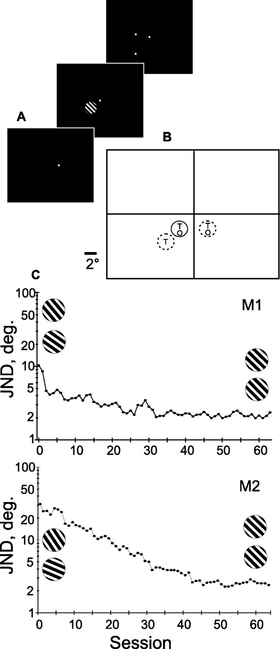
A, Training regimen. Subject fixated on a central red spot for 300 ms, followed by a 300 ms presentation of the stimulus. The stimulus then disappeared and the subject indicated the orientation by a saccade to one of the two target spots. B, Display screen and position of stimulus during training and behavioral testing. Solid outline, Trained and tested position. Dotted outline, Behavioral testing only. Letters “T” and “O” indicate where trained or orthogonal orientations were tested. The line segment at the lower left indicates scale. C, Staircase procedure training of monkeys 1 and 2. Each point is the average of all reversals for a daily session, which tends to be higher than the actual threshold. The orientations used in the testing in the first and last sessions are shown in inset: 130° compared with 140° and 134° compared with 136° for M1; and 119° compared with 151° and 134° compared with 136° for M2.

During the recording phase of the experiment, stimuli were centered on the receptive fields of the cells, the eccentricity of which ranged from 0 to 15°. Grating size and spatial frequency were approximately adapted for the eccentricity, using up to double the stimulus diameter and one-half the frequency for the most peripheral receptive fields tested. Sixteen stimulus orientations from 0 to 180° were tested at 11.25° intervals. Grating stimuli used during recording were otherwise identical with those used in training, except that the grating phase was fixed across trials.

Training.

The first two subjects were trained to discriminate small orientation differences around an oblique orientation of 135° using a staircase procedure. Stimuli were presented clockwise (CW) or counterclockwise (CCW) with respect to this reference. The subject was then required to indicate whether the grating presented was turned CW or CCW from the oblique by making a saccade to one of the two target spots that appeared ∼2° above and below the upper and lower stimulus borders. A correct response was rewarded with a drop of apple juice. No visible indication for the reference orientation of 135° was provided. Each staircase training session was initiated with a difference of 20° either side of 135°. The size of this difference was decremented by 20% after four successive correct responses or incremented by 20% after an incorrect response, to converge at a just-noticeable difference (JND) of 84% correct. After every 20 such reversals, the average JND was computed as the geometric mean of the 20 reversals, providing a continuous record of the subject's progress. After 40–60 daily sessions of up to 3000 individual trials each, subjects could easily discriminate orientations differing by <3° (1.5° either side of the oblique) with 84% accuracy (see Fig. 1 C). During the recording phase that followed, monkeys were given occasional “refresher sessions” to assure that learning was being retained and that any training effects remained strong. After completing the training and recording phases in monkey 2, JNDs were also determined using the same staircase procedure but at untrained orientations and spatial positions to assess transfer of learning to these other stimuli or positions. For these tests, the trained or the untrained (orthogonal) orientations were tested in the trained hemifield at both the trained and twice the trained eccentricity, and in the opposite untrained hemifield at the trained eccentricity, as illustrated in Figure 1 B.

Single-cell recording.

Extracellular recordings were made using sterile, tungsten-in-glass electrodes of ∼1 MÙ impedance. These were inserted transdurally with a hydraulic microdrive fixed to the recording chamber (David Kopf Instruments, Tujunga, CA) at an angle approximately normal to the cortical surface. Individual cells were isolated using a spike discriminator and spike events were stored at 1 ms resolution for later analysis. A typical daily recording session lasted 2–4 h. During actual recording, the monkey simply maintained fixation within a square, 1.5°-wide window, centered on a red spot on the screen while the stimuli were presented. Five hundred milliseconds after fixation onset, gratings of various orientations were presented for 300 ms with interstimulus intervals of 500 ms. The subject would continue receiving juice rewards and viewing stimuli for as long as he was able to maintain fixation, typically 10–20 s. Long fixation times were encouraged by gradually increasing the frequency of reward delivery during the course of each fixation period.

For each cell, a preliminary test was first performed to determine the size and position of the receptive field of the cell to be tested. The results of this test were used to center the stimulus on the receptive field and to determine whether or not the neuron gave a response at the trained position. Recorded neurons were classified as “trained” or “control.” A neuron was considered to be trained if preliminary testing indicated that its receptive field included a portion of the same region in visual space as the training stimulus. Control cells were recorded in the opposite hemisphere with respect to the training stimulus, and hence had receptive fields in the opposite quadrant of the visual field.

Over the course of our experiments, two methods were used for determining whether a receptive field overlapped with the trained position. In the very earliest experiments with monkey 1 (including 238 trained neurons from the final responsive and orientation-selective sample and none of the controls), this stimulus was a square, 1° flashed checkerboard of 2 cycles/deg that could be manually moved about the screen to any given coordinates, The receptive field borders were determined on-line by moving the flashing checkerboard around the screen, listening for responses, and noting coordinates where the response disappeared. Neurons were designated trained if any part of the trained position overlapped with the receptive field borders as determined by this method. In later experiments, a test was developed that systematically presented a flashed grating or checkerboard in an 8 × 6 grid (of ∼2° spacing, the “position test”) covering the visual quadrant being tested. Whether neurons were trained or not was determined off-line by calculating the average net firing rate for the four stimulus positions that overlapped the trained position. If this average was <10% of the average net firing rate at the optimal position of the test, the area occupied by the training stimulus was considered to lie outside the receptive field.

The next step was to determine the selectivity of the neuron for grating orientation with the “orientation test” consisting of the 16 orientations presented in random, interleaved manner. A neuron would nominally be tested with 30 presentations of the entire stimulus series unless the spike became lost or the quality of the recording began to degrade, as often happened during the 20–30 min period required to completely record a cell. Median and first and third quartiles over the final, orientation-selective population were 25, 15, and 30 presentations, per stimulus, respectively.

Data analysis.

Firing rates were calculated by counting spikes within a window beginning 50 ms after stimulus onset and extending to 50 ms after the end of the 300 ms stimulus. Net responses were obtained by subtracting average firing rates during the 300 ms periods preceding stimulus presentation (background activity) from these values. ANOVA was used to establish that firing rates in the stimulus window exceeded the firing rates during the prestimulus period and to assess the effect of the factor “orientation” on the responses. Except where mentioned (see Figs. 6, 7; Table 2), all analyses were performed on absolute firing rates.

Figure 6.

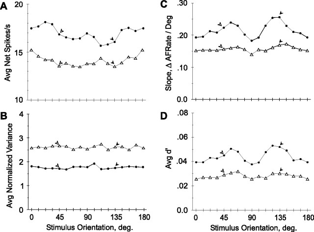
Neuronal response parameters as a function of stimulus orientation. Filled circles, Trained population; open triangles, control population. Filled and open arrowheads show positions of trained and orthogonal orientations, respectively. Same populations as in Figure 5 are shown. A, Net firing rate. B, Normalized variance. C, Slope of tuning curve. ΔAFRate, Change in average firing rate. D, d′. As explained in the text, a small percentage of responses were removed from C and D where the absence of any response could result in a division by zero.

Figure 7.

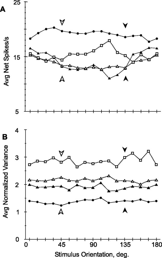
Neuronal response parameters as a function of stimulus orientation: individual hemispheres. A, Net firing rate; B, normalized variance. Dark symbols, Trained hemispheres; white symbols, control hemispheres; circles, triangles, and squares, M1, M2, and M3, respectively. Shown is the same population as in Figure 6.

Table 2.

Characteristics of trained and control populations of responsive V4 neurons

	Trained			Control
	Alln = 560 (416)	M1n = 327 (238)	M2n = 233 (178)	Alln = 578 (429)	M2n = 419 (310)	M3n = 159 (119)
SI
Mean	0.18	0.19	0.16	0.12	0.12	0.13
SD	0.18	0.20	0.14	0.12	0.12	0.13
Median	0.11§	0.11	0.11§	0.08	0.08	0.08
First quartile	0.06	0.06	0.06	0.04	0.04	0.04
Third quartile	0.23	0.23	0.23	0.16	0.15	0.20
MaxNFR
Mean	29.4	31.0	27.2	23.5	23.8	22.9
SD	23.3	25.6	19.6	15.2	15.6	13.9
Median	22.2§	22.8	21.4‡	20.2	20.4	17.7
First quartile	13.7	13.3	14.1	12.7	12.2	13.0
Third quartile	39.2	41.8	34.7	31.1	31.7	29.3
Fano
Mean	2.16	1.65	2.86	3.43	3.19	4.08
SD	2.44	1.88	2.98	3.04	3.02	3.03
Median	1.65§	1.27	2.26†	2.72	2.47	3.17
First quartile	0.98	0.76	1.48	1.70	1.54	2.16
Third quartile	2.63	2.00	3.38	4.11	3.83	4.60
Baseline
Mean	16.7	21.3	10.8	11.9	12.3	10.9
SD	19.9	23.1	12.6	11.3	11.8	9.9
Median	9.4§	13.3	6.2†	8.7	8.8	8.4
First quartile	3.0	4.3	2.0	4.3	4.0	5.1
Third quartile	22.0	32.4	13.7	15.9	16.5	13.5
Background firing rate
Mean	7.5	9.8	4.8	5.5	5.7	5.0
SD	8.8	10.0	6.1	4.7	5.0	3.6
Median	4.2§	6.4	3.1‡	4.3	4.3	4.5
First quartile	1.7	2.5	1.4	2.1	2.1	2.1
Third quartile	10.1	13.9	5.8	7.1	7.5	6.4

Response parameters of all neurons that responded significantly to the stimulus, including the selectivity index, net firing rate at the preferred orientation (MaxNFR) and Fano factor at the preferred orientation, the absolute firing rate at the least-preferred orientation (baseline), and the background firing rates when no stimulus was present. The number of neurons in each subsample are shown as well as (in parentheses) the number of cells for which the factor orientation gave a significant effect.

^§p < 10⁻⁵;

^†p < 0.05;

^‡p > 0.05 (NS); K–S test.

For most of the data analysis, only neurons for which both response and orientation were significant (p < 0.05) were considered, although some preliminary analysis used the entire population of neurons giving significant responses to the grating stimulus. In this case, histograms were constructed to show changes in basic response qualities including firing rate, response variance, and overall orientation selectivity. However, for the remainder of our analysis in which we looked for specific orientation-discrimination training effects, it made little sense to include cells conveying no information about orientation. Additional analysis was therefore confined to the neurons for which ANOVA showed the factor orientation to have a significant effect.

The strength of orientation tuning was quantified by a selectivity index (SI), where 1 equals complete selectivity with only one orientation responding and 0 corresponds to equal responses at all orientations. This is computed according to the following formula:

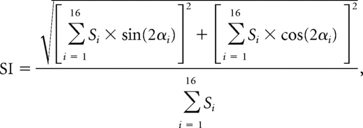where S_i is the absolute firing rate elicited at position i, and α_i is the angle of the orientation i. Similarly, the angular position of the maximum response, which characterizes the optimum or “preferred” orientation, is defined as follows:

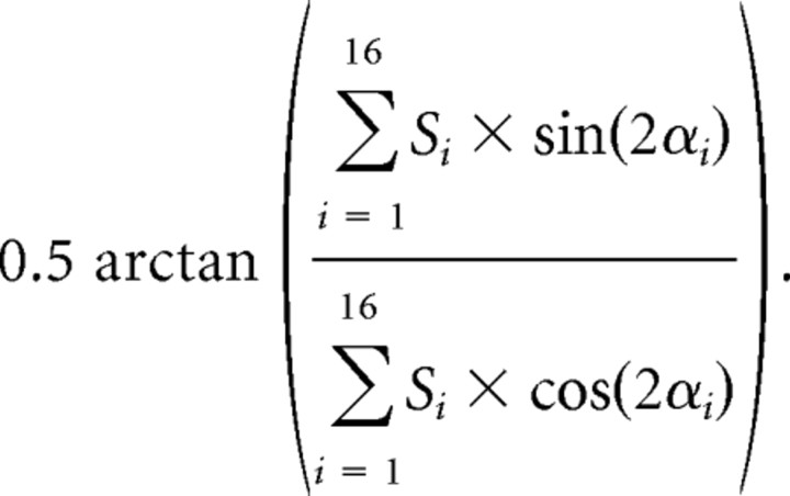Tuning curves were analyzed using methods similar to those of previous studies of perceptual learning in V1 (Schoups et al., 2001): The absolute responses were plotted as a function of orientation with the curve recentered so that the highest responses were at the center of the curve. The two values at each end of the curve were “wrapped” by copying them to the opposite ends to improve the accuracy of the fits near the ends of the curve. Finally, a sixth-order polynomial was fit to the response curves using a reiterative, least-squares method. Responses failing to produce an acceptable fit (r² < 0.6), ∼7–8% of both trained and control populations, were not further considered in this analysis. A sixth-order polynomial function was chosen rather than a Gaussian fit (Yang and Maunsell, 2004) because the polynomial curve is capable of detecting asymmetries in the tuning curves, and should provide a better fit. This indeed proved to be the case for a randomly selected sample of 50 V4 neurons for which the difference in fit was highly significant (paired t test, p < 0.0001). The choice of a sixth-order polynomial avoids the risk of overfitting that might result from the use of more flexible, higher-order polynomial curves.

For our purposes, the slope at any given point x on this curve was defined as the change in the absolute firing rate occurring over the interval between 1° to either side of the x value divided by the change in x (that is, 2°) over the same interval. From these slope values, we derive the value d′ at a particular orientation defined as follows: d′ = μ/ς, where μ is the change in mean firing rate, given in this case by the slope of the fitting function, and ς is the SD of the absolute responses at that orientation (Green and Swets, 1966). Because we expected increases in slope and d′ as a result of training, effects of training on these two parameters were tested with one-tailed t tests. Unless specified otherwise, the t test results refer to two-tailed t tests.

Much of the data analysis presented here follows one of two basic designs. The first, a “stimulus orientation” plot, averages some response parameter, such as firing rate, at each of the 16 orientations across all the cells in the population. This method was used to look for stimulus-specific effects that preferentially affected response parameters at the trained orientation in the trained population of neurons. The second analytical method, the “preferred orientation” plot was designed to uncover interactions between the trained orientation and the intrinsic tuning preferences of a cell, an approach similar to that used in previous investigations of perceptual learning (Schoups et al., 2001; Yang and Maunsell, 2004). For this type of analysis, each neuron was first assigned to one of 16 orientation categories based on its orientation preference, calculated as described above. These 16 groups were then combined, according to their distance from the trained or the orthogonal reference orientation, into three categories by lumping pairs of equidistant groups (on either side of the reference) together. Average response parameters within each group could then be calculated to determine whether the parameters of neurons with particular orientation preferences were preferentially affected by training.

Both the stimulus-orientation and preferred-orientation analyses were performed on neurons that were significantly orientation selective and for which the polynomial fit met the criterion. However, any analysis averaging data across all orientations of all cells will necessarily include points falling outside the response curve of a given cell. Some orientations will thus produce no response, particularly if the neuron shows strong tuning. Because this would result in a division by zero in calculating values such as normalized variance or d′, it was necessary to eliminate responses that were not at least equal to the spontaneous discharge rate (that is, were noninhibitory) and those averaging less than one spike per stimulus presentation. Applying these criteria removed only 10% of the total responses from the control and trained populations, but eliminated any undefined values from the analysis.

Schoups et al. (2001) used a Bayesian analysis to assess how reliably a population of neurons with orientation tuning curves such as those observed in the present experiment can signal small orientation differences at trained and orthogonal orientations. To be able to compare V4 with V1, we used exactly the same analysis as that performed by Schoups et al. (2001). This analysis assumes that variance equals mean firing rate, an assumption applying to only part of the present sample and to that of Schoups et al. (2001). However, it allows a direct comparison with the changes obtained earlier in V1 (Schoups et al., 2001). In neither study was any interaction found between orientation and variance; hence the two orthogonal orientations can be compared. The procedure estimates the probability that a population of neurons can correctly signal which one of two possible orientations has been presented (Oram et al., 1998; Schoups et al., 2001), based on the response curve of the cell as represented, in this case, by the fitted polynomial curve. The average firing rates derived from this curve are used to generate simulated responses, modeled as a Poisson process, at each orientation. Each simulated response has in turn a certain probability, which can be estimated from the Poisson probability density function, of having been elicited by a given orientation. For a population of cells, we can apply Bayes' rule to combine their individual probabilities to obtain the probability that the population has signaled a particular orientation, given that particular set of responses. To compare how accurately sample cell populations can signal orientations at the trained and orthogonal orientation, we examined pairs of orientations lying close to these reference orientations. In practice, orientations lying within 5° of the reference orientation were chosen, thus testing selectivity over a 10° range centered on either the trained or control orientations. Orientation differences encompassing 1, 2, 3, 4, 5, 6, 8, and 10° were tested in this manner. For each these 8 points, 30 random samples of 20 neurons were drawn with replacement from the cell population. Each of the samples of 20 neurons was tested with 2000 simulations performed using the orientation difference for that point; thus, each point represents some 60,000 simulated sample responses. As described above, each simulated stimulus presentation resulted in a probability that one of the two orientations in the pair had been presented, given the responses generated by the set of neurons. By scoring each of these 60,000 simulations as “correct” or “incorrect,” it was possible to tally the percentage of correct discriminations, thereby quantifying the ability of the population to discriminate between a given pair of orientations.

Results

Two monkeys were extensively trained in discriminating small differences in orientation around 135° at a fixed parafoveal position. To detect changes in the response properties of V4 neurons resulting from this training, we compared the responses of V4 neurons in trained and control hemispheres of three monkeys while the animals performed a simple fixation task. We will first describe relevant behavioral results, and then discuss modifications in the neural response consequent to training.

Behavioral training and behavioral testing

Our two trained subjects required 35–50 sessions of up to 3000 individual stimulus presentations per session to arrive at their minimum thresholds (Fig. 1C). These animals showed dramatic improvement in their ability to distinguish orientations near 135° after training. Initially able to distinguish only differences greater than ∼10 or 20°, both subjects eventually achieved thresholds in the range of 2.0–2.4 (1.0–1.2° either side of the trained orientation). Behavioral testing performed in monkey 2 after recording had been completed, showed that the observed improvements in threshold, measured as the JND, were transferred poorly to other orientations or spatial positions (Table 1), as previously found for orientation discrimination tasks of this type in humans (Vogels and Orban, 1985; Schoups et al., 1995) and monkey subjects (Schoups et al., 2001). For the orthogonal orientation, or for the trained orientation but at higher eccentricity and in the opposite hemifield at the same eccentricity, thresholds averaged close to 13°, much higher than the 2° observed at the trained orientation and position. Nonetheless, a significant difference could be discerned between the trained and the control hemisphere for the untrained orientation. It seemed reasonable that taking the subject's best, rather than average, performance at any given position or orientation will provide the most valid estimate of the performance limit for that condition, because this would limit the influence of irrelevant factors such as motivation or unfamiliarity with the particular task. To estimate this best discrimination ability, we selected the 10 smallest of the 80 or so 20-reversal averages obtained for each condition. For this criteria, untrained orientation conditions in the trained hemisphere consistently gave significantly smaller JNDs (mean, 8.5°) than the control hemisphere (mean, 11.8°; p < 0.001, t test).

Table 1.

Thresholds measured at various locations and orientations

	135°	45°	135°, ecc.
Trained hemifield
Average	2.5	13.1	12.8
High	1.9	8.5	11.1
Low	3.0	14.5	14.6
Control hemifield
Average	13.6	13.3
High	12.1	11.8
Low	14.5	14.3

Thresholds as the JND, measured at the trained (135°) and control (45°) orientations, in the trained and control hemifields, and at the trained orientation, but at twice the eccentricity (135°, ecc). The average is for all reversal points of the staircase. The high and low are the averages of the 10 highest and 10 lowest sets of 20 reversals. Data were obtained from monkey 2 after the recording had been terminated.

Neuronal responses: general

We recorded data from over 1200 neurons in our three monkeys at eccentricities ranging from 0 to 15°. Medians, and first and third quartiles (in parentheses) of eccentricities for trained and control populations were 4.1° (3.3°, 6.6°) and 5.3° (4.1°, 6.6°), respectively. Although small, this difference was nonetheless significant (p < 3 × 10⁻⁵). The vast majority (1138 cells, including 560 trained and 578 control neurons) gave significant responses (ANOVA) to the gratings (for breakdown per monkey, see Table 2). Of these, 845 (416 trained and 429 control) also showed a significant orientation effect and gave an acceptable fit using a sixth-order polynomial function. These 845 neurons constituted the main sample population used in the analysis presented below. Figure 2 illustrates a fairly typical response from a cell recorded in area V4 of monkey 3. This example was a well tuned neuron recorded at 3.5° eccentricity, giving a maximum average firing rate of 47 spikes/s to the 101° grating. It had a preferred orientation and SI, calculated from circular statistics, of 97 and 0.71, respectively, and the polynomial fit (r² = 0.98) indicated a half-height tuning width of ∼70°. Although the stimulus variable orientation produced a significant effect in the vast majority of the neurons tested, not all showed the degree of tuning illustrated by this neuron. Previous investigators have noted that only about one-half (Schein et al., 1982) to two-thirds (Desimone and Schein, 1987) of V4 neurons display strong orientation tuning. For our analysis, any cell for which the factor orientation was significant in an ANOVA was included in the analysis, because all such neurons were at least theoretically capable of encoding the orientation of the stimulus. Of the 845 neurons meeting the ANOVA criteria, 693 (82%) were tuned to the extent that their fitted curve fell to <50% of the maximum value at the minimum of the curve.

Figure 2.

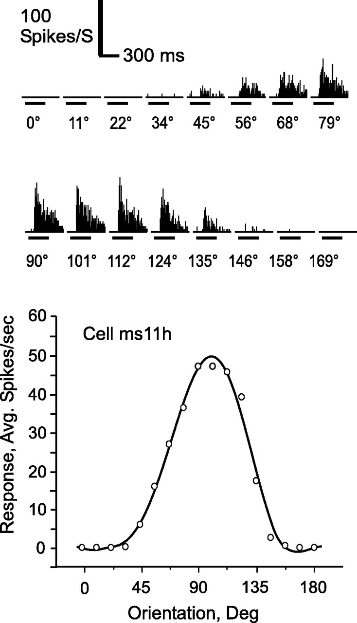
Response to grating stimulus in typical V4 cell. Histograms (above) show cumulative responses to the 16 tested orientations. Time course and strength of responses are indicated by the scale. The lower panel shows the same data, calculated as average absolute firing rate, recentered, and fit with polynomial curve. By definition, 0° is horizontal.

Nonspecific or general neuronal effects of training

Before isolating the orientation-selective cells for additional analysis, it was informative to first look at certain parameters relating to the orientation selectivity of the entire population (n = 1138). We determined the firing rate and variance for the maximum response, and calculated the orientation selectivity, measured by the SI, of all neurons in the trained and control populations for which ANOVA indicated a significant response. We found an increase of 20% in the average maximum net firing rate of the trained population compared with the control population (Table 2). Expressed as medians, this corresponds to a 10% increase, close to previously reported increases in neuronal firing rates in V4 cortex after training in a discrimination task (Yang and Maunsell, 2004). The difference in mean firing rate between trained and control population was even larger for the maximum absolute firing rate (36.9 vs 29 spikes/s; Kolmogorov–Smirnov (K–S), p < 0.001). However, differences in maximum net and absolute firing rates were not significant in monkey M2 (p > 0.1, K–S) and hence the differences between trained and control population mainly reflect differences between animals.

Next, we compared the SI in the trained and control populations (Fig. 3A). Here, too, there was a significant (p < 0.001, K–S) training effect that could not be explained by eccentricity [p < 10⁻⁶, analysis of covariance (ANCOVA)]. The histogram clearly shows the 30% increase in the mean SI among the neurons in the trained population. Differences between trained and control neurons proved consistent across animals. In particular, the differences in SI remained significant (p < 0.00002, K–S) when trained and control neurons were compared within a single subject (monkey 2). Yang and Maunsell (2004) reported a corresponding 12° (13%) decrease in the average full-width bandwidth of Gaussian curves fitted to normalized firing rates of trained versus control neurons. The two results cannot be directly compared, because a polynomial fit has no parameter corresponding to bandwidth, but we could use the points where the response falls to 50% of the maximum to estimate bandwidth. This method gave estimates of 84 and 78° (p < 0.001, K–S) for average full-width bandwidths in control and trained populations, respectively. This corresponds to a decrease of 7%; thus, changes are approximately similar to those reported by previous investigators despite the use of dissimilar analytical techniques.

Figure 3.

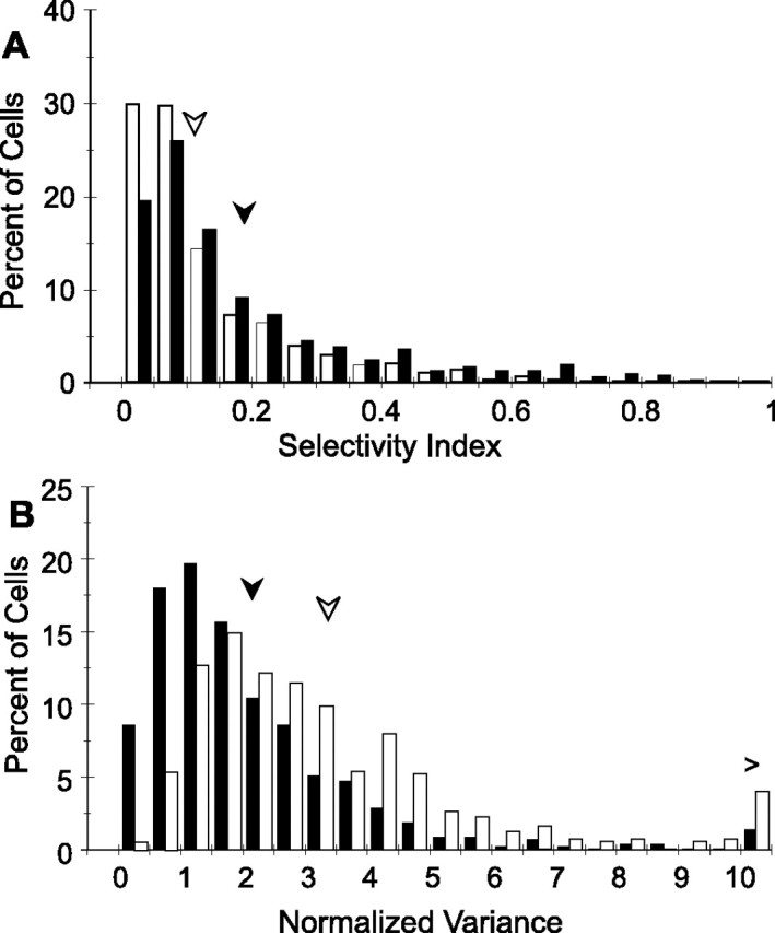
Histograms comparing response parameters in trained and control populations in all neurons giving a significant response to the grating stimulus. n = 560 and 578 for trained and control populations, respectively. Filled bars, Trained neurons; open bars, control neurons. Filled and open arrows indicate corresponding means. A, Selectivity indices in trained and control neurons. Means (medians) of distributions are 0.18 and 0.12 (0.11 and 0.08) for trained and control, respectively. B, Population variance as Fano factor or normalized variance, at preferred orientation. Means (medians) are 2.2 and 3.4 (1.6 and 2.7) for trained and control. For both comparisons, p < 0.001 (K–S).

The variance must first be known if single-cell performance is to be related to behavioral performance (Vogels et al., 1989; Seung and Sompolinsky, 1993; Ghose et al., 2002), because any decrease in response variance, assuming other response parameters remain constant, will increase the ability of that neuron to discriminate between similar stimuli (Green and Swets, 1966; Pouget et al., 2003). To determine whether the observed increase in firing rate within the trained population was accompanied by a change in the variance, we calculated the variance normalized to the spike count, or Fano factor, at the preferred orientation of each cell. Figure 3B illustrates the substantial 37% decrease in the mean normalized variance of the population, from 3.43 to 2.16 (p < 0.001, K–S; p < 2 × 10⁻⁵, ANCOVA controlling for eccentricity). This difference even remained significant when only monkey 2 was considered (Table 2) (p < 0.05, K–S). Comparing the geometric rather than the arithmetic means yielded equally significant differences: 2.70 compared with 1.59 (p < 10⁻⁶, t test).

Because the values plotted in Figure 3B were normalized to response, however, the observed difference could have been attributable to either a decrease in the variance per se or to changes in the mean response, with no change in mean variance. Additional analysis was therefore necessary to examine the relationship of these two factors over the full range of responses. It has been shown that log variance increases nearly linearly with log response strength, as a power function with a value close to 1 (Vogels et al., 1989). The corresponding power of the fitted power functions for our trained and control populations were 1.01 and 1.29 (p < 0.001, t statistic comparing slopes), respectively (Fig. 4). The baseline variance, given by the y-intercepts, was nearly identical, but variance did not increase as quickly for higher response rates within the trained population as it did in controls. This result held whether we compared all cells or only the orientation-selective cells, whether we plotted responses to all orientations or only the response of each cell at the preferred orientation (as in Fig. 4), and even whether we compared trained and control populations recorded within the same animal (monkey 2; t statistic comparing slopes, p < 0.001). This effect was also observed if, rather than analyzing the relationship between log variance and log average response across cells, we examined this relationship for individual neurons. The mean slopes of these linear functions were 1.02 and 1.26 for trained and control neurons, respectively (supplemental Fig. S1, available at www.jneurosci.org as supplemental material), a highly significant difference (p < 0.001, K–S). Intercepts were not significantly different. Similar results were obtained when only the neurons recorded in monkey 2 (supplemental Fig. 1, available at www.jneurosci.org as supplemental material) were considered, and the slope was significantly reduced in the trained population (p < 0.01, K–S). The lower variance in the trained population would tend to increase the orientation discriminability in these neurons, assuming that other factors, including response strength and bandwidth, remained constant. We could find no relationship between variance and either the stimulus orientation or the preferred orientation of the cells, and thus we regarded this aspect of our findings as nonspecific with respect to orientation.

Figure 4.

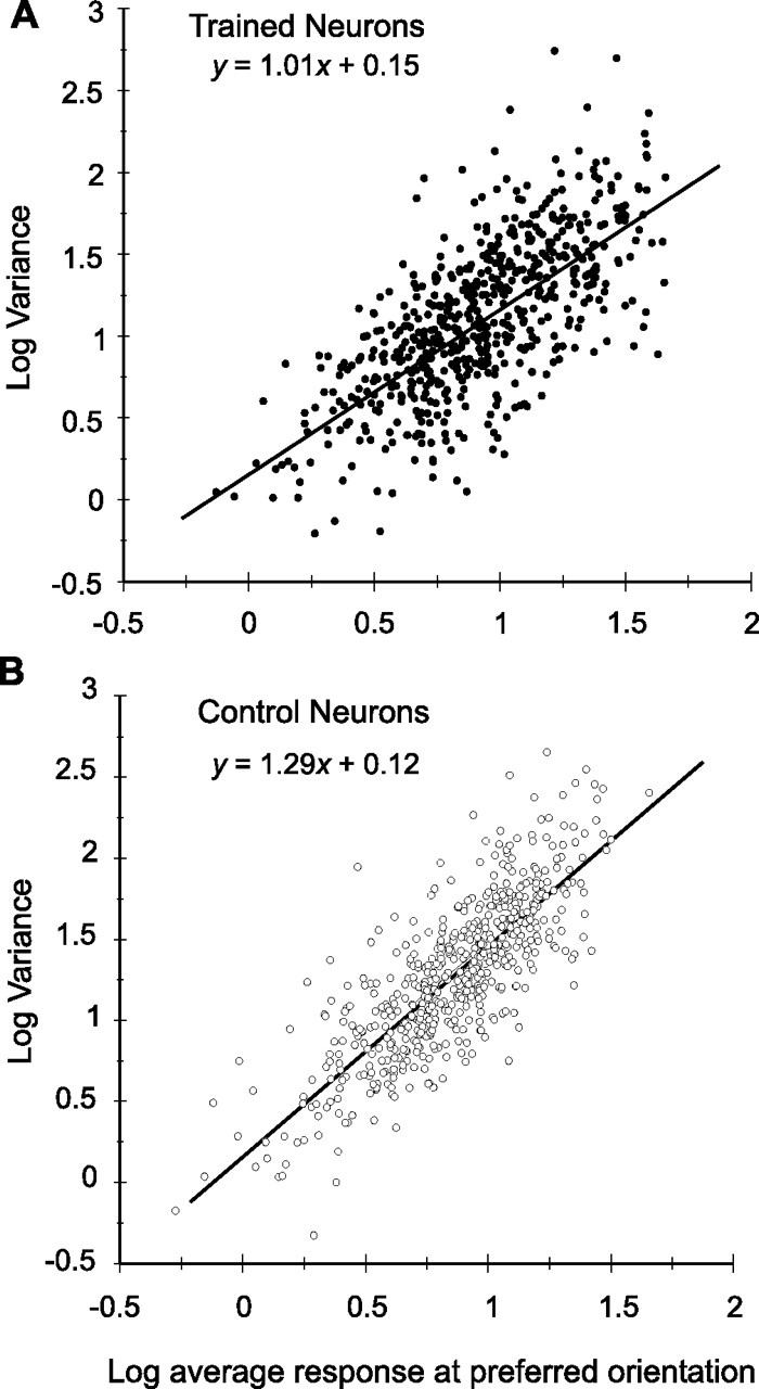
Same populations as in Figure 3, plotting log variance as a function of log response strength at the preferred orientation and fitting a linear regression line using least-squares method. Slopes of the two plots (1.01 and 1.29 for trained and control, respectively) were significantly different from one another (p < 0.001, t statistic).

The nonspecific aspect of changes in variance was further illustrated by a subset (95 trained and 104 control neurons) of the cell population described in Figures 3 and 4 and in Table 2. Neurons were selected that had shown no effect of orientation on firing rate in the original ANOVA testing the effect of orientation. Any effects within this population would therefore, by definition, be nonspecific with regard to stimulus orientation. The mean normalized variance (Fano factor) in the control population of 3.0 was significantly higher (p < 10⁻⁶, ANOVA) than the mean variance in the trained population at 2.4.

Stimulus orientation and orientation-specific neural training effects

To look for effects associated with particular stimulus orientations or among cells with particular orientation preferences, we selected for further study the neurons for which ANOVA had demonstrated that the variable orientation produced a significant effect on the response (n = 845). The analysis performed on this population closely followed the methodology of a previous publication (Schoups et al., 2001) from our laboratory, with two major changes: tuning curves were not normalized before averaging and the effects of variance were included by calculating not just the slope of the tuning curves but also the d′.

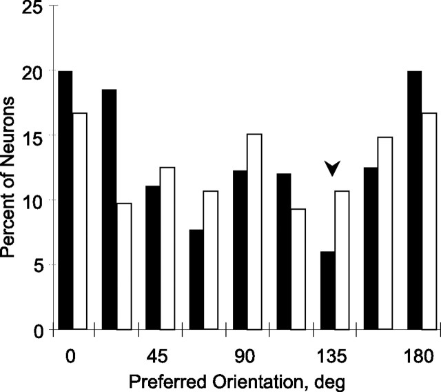
Previous studies have shown decreases in the number of cells preferring the orientation of an extensively trained stimulus, in both macaque V4 (Yang and Maunsell, 2004) and V1 (Schoups et al., 2001; Ghose et al., 2002). We also found a significant (p < 10⁻⁶, K–S) deviation from uniform distribution of the preferred orientations (Fig. 5) in the trained but not the control population, where the distribution was statistically equivalent to a uniform distribution (p > 0.10, K–S). The difference in distributions of preferred orientation between trained and control neurons was significant both in a 2 × 8 χ² test (χ² = 24; p < 0.001) and the Watson–Williams test comparing mean orientations (F_(1,844) = 10.3; p < 0.002). Even when the comparison was restricted to monkey 2, the difference in distributions remained significant (χ² = 15.9, p < 0.05; and F_(1,487) = 44.6; p < 0.001).

Figure 5.

Histogram of preferred orientations in all V4 neurons giving significant response, effect of orientation, and polynomial fit (n = 416 and 429 for trained and control neurons, respectively). Filled bars, Trained neurons; open bars, control. The arrow shows the position of trained orientation. The distribution of the trained population differs significantly from a uniform distribution (p < 10⁻⁶, K–S), which was not the case in the control population (p > 0.10).

Discriminative performance of a group of neurons is not governed solely by the population size but also depends on a number of tuning characteristics. Therefore, we examined a number of tuning parameters, relevant for discrimination, as a function of stimulus orientation, including firing rate, response variance, the slope of the tuning curve, and the d′ of the response. As expected from the changes observed in the general population of responsive neurons, there was a significant (p < 0.025, ANOVA) difference between the net firing rates in the trained and control populations of orientation tuned neurons (Fig. 6A) that again could not be explained as any eccentricity effect (p < 10⁻⁶, ANCOVA). However, considering net firing rate in the individual hemispheres revealed large differences between the trained hemispheres of monkeys 1 and 2 (Fig. 7A). Furthermore, restricting the comparison of trained and control populations to monkey 2 failed to reveal a significant overall increase in net firing rate (p > 0.3, t test). The response variance did not depend on stimulus orientation in either the trained or control population (Fig. 6B) (p > 0.7 and 0.9, paired t tests, trained vs orthogonal orientations in trained and control populations, respectively). There remained only the strong but nonspecific effect between populations, with means of 1.7 and 2.6 (p < 10⁻⁶, ANOVA) in trained and control populations, respectively. In contrast to the changes in firing rate, the changes in normalized variance remained consistent across the four hemispheres and the difference between trained and control populations within monkey 2 was nearly significant (p = 0.052, t test) (Fig. 7B).

Figure 6C shows the average tuning curve slope plotted as a function of stimulus orientation. Both theoretical studies (Seung and Sompolinsky, 1993) and our previous results in V1 (Schoups et al., 2001) predict higher slopes at the trained compared with the orthogonal orientation, hence the use of a one-tailed t test. Comparing slopes at the trained and orthogonal orientations revealed a significant (p < 0.025, one-tailed paired t test) steepening of the slope in the vicinity of the trained orientation in the trained population that was not present in the control population (p > 0.1, one-tailed paired t test). Moreover, the signed differences between trained and orthogonal orientations showed a significant “difference of differences” between the trained and control populations (p < 0.02, one-tailed t test). Here, too, an apparently nonspecific effect appeared between average slopes in the trained and untrained population, with mean slopes of 0.22 and 0.16 spikes · s⁻¹ · deg⁻¹, respectively (p < 0.005, one-tailed t test; p < 10⁻⁶, ANCOVA with eccentricity as covariate). Considering the effects of stimulus orientation on the slope of the tuning curves in the individual hemispheres (Fig. 8A) revealed that the specific effect was present in the two trained hemispheres, reaching significance in monkey M1 (p < 0.05, one-tailed paired t test), but falling just short of significance in monkey M2 (p = 0.07, one-tailed paired t test). The aspecific effect was mostly attributable to interindividual differences, and the difference in slope across orientations between the trained and control hemisphere of M2 was not significant (p > 0.3, one-tailed t test).

Figure 8.

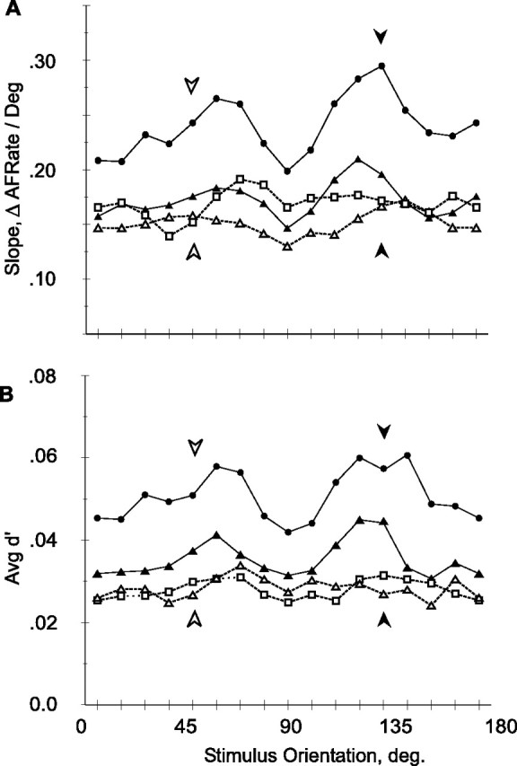
Neuronal response parameters as a function of stimulus orientation: individual hemispheres. A, Slope of tuning curves. ΔAFRate, Change in average firing rate. B, d′. Dark symbols, Trained hemispheres; white symbols, control hemispheres; circles, triangles, and squares, M1, M2, and M3, respectively. Shown is the same population as in Figure 6.

Note that the slope and d′ exhibit a secondary maximum at 54° in addition to that around 135°. This secondary maximum may be related to the slightly better discrimination at the untrained orientation in the trained hemisphere compared with the untrained hemisphere (Table 1). This local increase in slope probably reflects both the increase in the number of neurons tuned to cardinal orientations (Fig. 5) and stronger responses of these neurons. Indeed, neurons preferring horizontal or vertical orientations responded significantly more strongly than those tuned to oblique orientations in the trained (t test, p < 0.05) but not in the control population. The orientation anisotropy is thus much stronger in the trained population compared with the untrained control. A small anisotropy was also present in another V4 sample (Mysore et al., 2006) and inferotemporal cortex neurons also show a strong bias in their orientation preferences toward cardinal orientations in monkeys trained in orientation discrimination (Vogels and Orban, 1994). Although the present training started with distinction between vertical and horizontal orientations, it is unlikely that this explains the strong orientation anisotropy observed in the trained population, because the monkeys' performance improved rapidly (Fig. 1C) and orientations much closer to 135° were then presented.

The data showed an orientation-specific effect on slope, whereas the variance remained remarkably constant across all orientations. It therefore follows that the d′, which is simply slope divided by the SD of the responses, should show an orientation-specific effect similar to that of the slope. This was indeed the case, as illustrated by Figure 6D. As with the slope, the average d′ in the trained population was significantly higher around the trained orientation compared with the orthogonal orientation (p < 0.005, one-tailed paired t test). This was not the case in the control population (p > 0.2, one-tailed paired t test), and the trained and control populations were significantly different from one another, with regard to the magnitude and sign of these orientation-specific differences (p < 0.05, one-tailed t test) and with regard to average values across all orientations (mean d′, 0.044 and 0.028; p < 10⁻⁶, one-tailed t test). Again considering the individual hemispheres revealed that the orientation-specific changes in d′ were consistent across the two trained animals (Fig. 8B), and reached significance both in M1 and M2 (p < 0.03 and p < 0.0005, respectively; one-tailed paired t test). Furthermore, taking the difference in the d′ at the trained and at the orthogonal orientations of each cell yielded significantly (p < 0.01, one-tailed paired t test) different values for the trained and control hemispheres of M2.

Preferred orientation and specific neural training effects

One of the more compelling findings to emerge from our previous investigations into perceptual learning has been the discovery that training selectively affects the V1 neurons most sensitive to orientation changes near the training stimulus (Schoups et al., 2001). To investigate whether changes were similarly selective in V4, we subdivided the data shown in Figure 6 for the trained (135°) and orthogonal (45°) orientations, according to the angle between the preferred and trained/orthogonal reference orientations. To maintain enough power for statistical testing, we restricted ourselves to three groups of preferred orientation, relative to the reference orientation (trained or orthogonal) (Figs. 9, 10). These analyses were restricted to those parameters that showed orientation-specific training effects that were consistent across subjects [i.e., slope (Fig. 9) and d′ (Fig. 10)].

Figure 9.

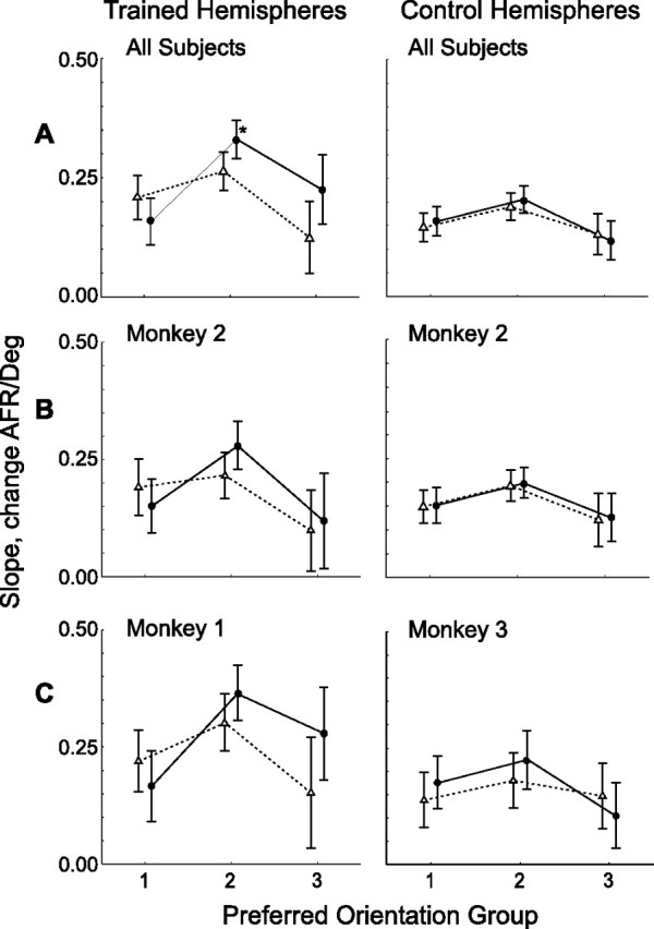
Slope of tuning curves at trained (solid lines; filled circles) and orthogonal (dotted lines; open triangles) orientation plotted as a function of preferred orientation groups, relative to reference orientation (trained or orthogonal orientation). Trained and control hemispheres, Plotted left and right columns, respectively. A, Overall populations. Shown are the same populations as in Figure 6. B, Monkey M2; C, monkeys M1 and M3. Neurons were grouped according to their preferred orientation, determined by circular statistical methods, and average slope was calculated for each orientation group. Error bars are 95% confidence intervals. Group 0, Preferred orientation 0–33° from reference; group 1, 34–67° from reference; and group 2, 68–90° from reference. Asterisk indicates conditions significant in post hoc analysis (Fisher's LSD, <0.05). AFR, Average firing rate.

Figure 10.

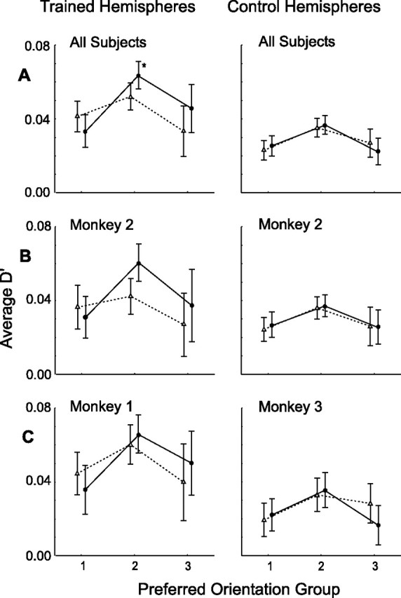
d′ at trained (solid lines, filled circles) and orthogonal (dotted lines, open triangles) orientation plotted as a function of preferred orientation groups, relative to reference orientation (trained or orthogonal orientation). Trained and control hemispheres, Plotted left and right columns, respectively. A, Overall populations. Shown are same populations as in Figure 6. B, Monkey M2; C, monkey M1 and M3. Neurons were grouped according to their preferred orientation, determined by circular statistical methods, and average slope was calculated for each orientation group. Error bars are 95% confidence intervals. Shown are the same groups as in Figure 10. Asterisks indicate conditions significant in post hoc analysis (Fisher's LSD, <0.05)

The average slope of the tuning curve at the trained and orthogonal orientations is shown for the three preferred-orientation groups, plotting trained and control populations separately (Fig. 9A) for sake of visibility. A factorial ANOVA showed a significant (F_(2,1554) = 3.9, p < 0.03) three-way interaction between the factors “trained/control population,” “trained/orthogonal orientation,” and “orientation preference group” (main effects: “hemisphere,” F_(1,1554) = 20.8, p < 10⁻⁶; “orientation group,” F_(2,1554) = 25.3, p < 10⁻⁶; “trained/untrained orientation,” F_(1,1554) = 2.8, p < 0.1). Moreover, the interaction of trained/orthogonal orientation and orientation preference group was also significant in the trained hemisphere (F_(2,749) = 4.4, p < 0.02). Post hoc testing indicated that the orientation-specific increase in slope was restricted to orientation preference group 2 (i.e., neurons with preferred orientations 34–67° away from the reference) [p > 0.1, p < 0.03, and p > 0.06, Fisher's least significant difference (LSD) test for groups 1, 2, and 3, respectively]. Analysis of the individual hemispheres (Fig. 9B,C) indicated that the effects in the trained hemispheres of M1 and M2 were similar and also that the difference between trained and control hemispheres was also present in M2. Unfortunately, the limited number of neurons in the different groups/animals prevented these differences from reaching significance.

To see how such changes translated into discrimination capacity, we performed an identical analysis on the average d′, measured at the trained and orthogonal orientations, for neurons grouped according to orientation preference in trained and control populations (Fig. 10). ANOVA again revealed a significant (F_(2,1554) = 3.2, p < 0.05) three-way interaction between trained/control population, trained/orthogonal orientation, and orientation preference group (main effects: hemisphere, F_(1,1554) = 49.6, p < 10⁻⁶; orientation group, F_(2,1554) = 26.7, p < 10⁻⁶; trained/untrained orientation, F_(1,1554) = 1.2, p < 0.3). Moreover, there was a significant interaction (F_(2,749) = 3.2; p < 0.05) between trained/orthogonal orientation and orientation preference groups in the trained population (Fig. 10A), but not in the control population. Again, the training effects were restricted to neurons with orientation preferences between 34 and 67° from the trained orientation and post hoc testing indicated that the difference in the d′ at the trained and untrained orientations reached significance only in orientation preference group 2 (p > 0.15, p < 0.03, p > 0.15; Fisher's LSD test for groups 1, 2, and 3, respectively). Considering the individual hemispheres again revealed similar training effects in both monkey M1 and M2, although the effect in M1 was stronger in orientation group 3 than in group 2 (Fig. 10C). Also, the effect of training could be clearly seen within M2, but, here too, the numbers of neurons were too small for these differences to reach significance.

Localized changes of the orientation tuning curves

Although data analysis based on both the stimulus orientation and the preferred orientation of the neurons indicate that tuning curves were modified in a highly specific manner, the analysis to this point still leaves open two possibilities. The increase in slope in select cell populations results either from a symmetrical narrowing of the tuning curves, or from a localized and asymmetric modification of these response functions. To address this issue, we compared the slope at the trained orientation with that of the symmetrically opposite point on the other side of the preferred orientation. For example, for a neuron having a preferred orientation of 100°, the slopes at 135 and 65° were taken. Slopes were significantly (p < 0.025, paired t test) higher on the side of the trained orientation (0.26 spikes · s⁻¹ · deg⁻¹) than on the opposite side (0.23 spikes · s⁻¹ · deg⁻¹). To determine whether particular orientation groups were selectively affected, we considered four groups of orientation preference, relative to the trained orientation (Fig. 11). The effect was strongest among neurons having preferred orientations between 22 and 67° from the trained orientation (p < 1.5 × 10⁻⁴, paired t test; for individual groups, 0–22, 22–45, 45–67, and 67–90°; significance levels were p > 0.30, p < 0.002, p < 0.025, and p > 0.20) (Fig. 11).

Figure 11.

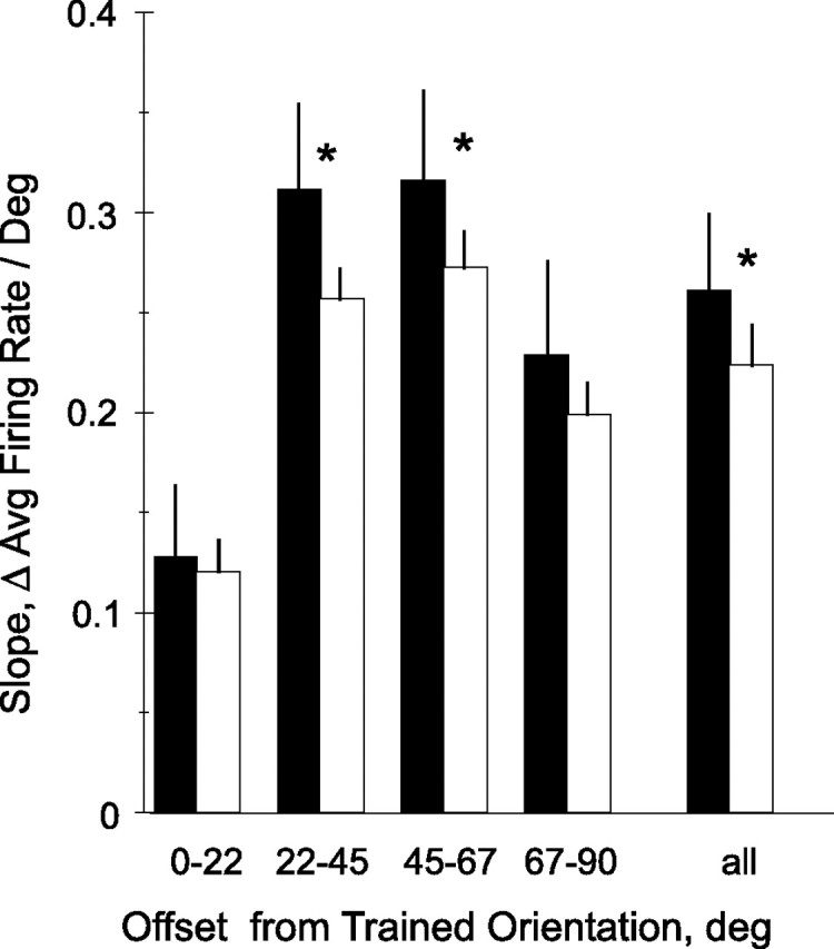
Slopes of orientation tuning curves by relationship to trained orientation. Slopes were measured, for the tuning curve of each neuron, at the trained orientation (filled bars) and at the symmetrical position (with respect to the preferred orientation) on the side opposite the trained orientation (open bars). Neurons were then grouped according to how far the preferred orientation lay from trained orientation (x-axis). Error bars are SEM; asterisks indicate conditions where trained and opposite sides were significantly different (p < 0.05, paired t test).

To visualize the asymmetry of the orientation tuning curve after training, we averaged the curves after aligning them on their preferred orientations. Given the differences as function of the orientation preference group, we considered the neurons with preferred orientation lying between 22 and 67° from the trained orientation separately from the other neurons in the trained population. The resulting average tuning curves are shown in Figure 12, with the trained orientation by convention placed on the right of the preferred orientation. For purpose of comparison, the left side of the curve, corresponding to orientations on the opposite side of the preferred orientation relative to the trained orientation, has been mirrored about the preferred orientation and drawn as a dashed line. The curves are asymmetric for trained neurons with preferred orientations within 22–67° from the trained orientation (Fig. 12A), but not for the remaining trained neurons outside that range (Fig. 12B) nor for the control neurons (Fig. 13C,D). Notice the higher firing rates in the trained neurons with preferred orientation within 22–67° from the trained orientation, which includes the neurons tuned to horizontal and vertical orientations (see above). The difference in the average responses 45° clockwise and counterclockwise from the preferred orientation in Figure 12A is highly significant (p < 0.0025, paired t test). Plotting the curves of trained neurons with preferred orientations between 22 and 67° to the left (Fig. 12E) of the trained orientation separately from those to the right (Fig. 12F) yields curves with opposite asymmetries (Fig. 12D), despite small differences in background firing rate, maximum net firing, and tuning width. Finally, restricting the analysis of the trained neurons with orientation preferences 22–67° from the trained orientation to individual monkeys still yields an asymmetric average tuning curve. The difference in pairs of responses 45° clockwise and counterclockwise from the preferred orientation proved significant (paired t test, p < 0.025, and p < 0.05 for M1 and M2, respectively).

Figure 12.

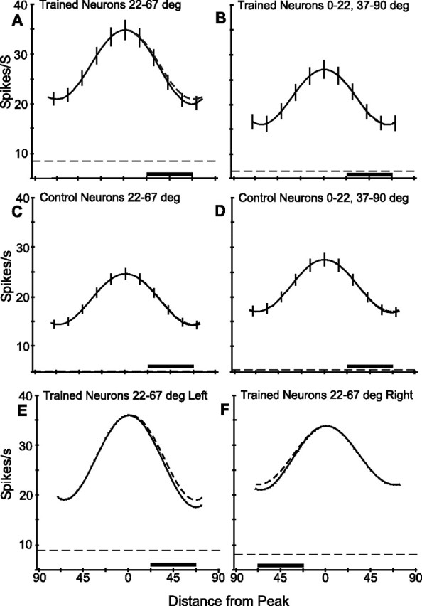
Average tuning curves of V4 neurons. A, Trained neurons with preferred orientations lying 22–67° from trained orientation (n = 261). B, Remaining trained neurons (n = 155) with preferred orientations between 0 and 22° or 67 and 90°. C, Control neurons with orientation preferences in the same 22–67° range (n = 247) as those in A. D, Control neurons with orientation preferences in the 0–22° and 67–90° ranges (n = 182). E, F, Trained neurons with preferrred orientations 22–67°, as in A, but separating those with their peaks lying to the left (E; n = 101) or right (F; n = 160) of the trained orientation. Vertical lines (in A–D) show SEM at representative orientations; dashed curves (in A, and E and F) are simply the opposite side of the same curve reflected over, to facilitate comparison. The solid horizontal lines near the bottom show the ranges containing the trained orientation for these neurons. The dashed horizontal lines show average background activity (note that y-axis begins at 5, not 0).

Figure 13.

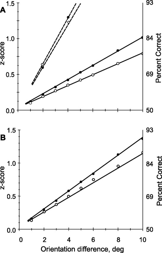
Neuronal performance as calculated using Bayesian analysis. Top panel, Analysis of entire trained (n = 416) population, z-transformed data fit with linear regression using method of least squares. Filled circles, Trained orientation; open circles, orthogonal orientation. Slopes are significantly different (p < 0.001, t statistic). The difference represents a 28% improvement in the trained population. Dotted lines show results from V1 (Schoups, 2001) added for comparison. Although slope here is much steeper, because of narrower tuning curves, improvement is only ∼7%. B, Comparison considering only neurons with preferred orientations between 30 and 50° from trained orientation, placing trained orientation on the flanks of the curves. Regression lines are steeper than in A.

Quantifying orientation discrimination using Bayesian analysis

Finally, to compare orientation training effects in V4 with the results of similar studies in V1 (Schoups et al., 2001), we also performed a Bayesian analysis using the methods of that study. This analysis quantifies the ability of a neuronal population to discriminate between small changes in stimulus parameters given the average response of individual cells derived, in this instance, from the response values indicated by the fitted tuning curve. Because the Schoups et al. (2001) implementation assumes equal variances, and because we have already shown that the variance differs between trained and control populations, analysis must be confined to intrahemispheric comparisons. Figure 13A shows that, for neurons in the trained population, there was a considerable (p < 0.001, t statistic comparing slopes of regression lines) difference in discrimination ability at the trained and the orthogonal orientations. In contrast, slopes at the trained and orthogonal orientations in the control population were statistically indistinguishable (p > 0.50, t statistic). Data and fitted regressions for V1 from the report by Schoups et al. (2001) were plotted on the same axes for comparison. The steeper regression slopes in V1 were a consequence of the much narrower average tuning curves in the primary visual area compared with V4. The regression lines for the trained and orthogonal orientations showed that the training effect in V4 represented about a 28% improvement in orientation resolution. This value considerably exceeded the 7% reported by Schoups et al. (2001) for V1. Figure 13B considers only V4 neurons with preferred orientations in the most strongly affected range of 30–50° from the trained orientation. The improvement in orientation discrimination is about the same as that in the overall population, but the resulting slope is much higher, indicating that these cells are more sensitive to small changes in orientation near the trained orientation. Effects were consistent across monkeys (supplemental Fig. 2, available at www.jneurosci.org as supplemental material), especially when the neurons with the steepest slopes are considered.

Discussion

Extensive training in an orientation discrimination task resulted in significant changes in the response properties of V4 neurons. Neurons in the trained hemisphere showed decreased response variance and narrower orientation tunings compared with the untrained hemisphere. In the vicinity of the trained orientation, average neuronal tuning curves showed local increases in the slope of the tuning curve, leading to an increase in discriminability around the trained orientation. The increases in slope and discriminability were restricted to the most informative neurons, those with preferred orientations offset by some 25–65° from the trained orientation. Slope increases among these neurons were confined to the portion of the orientation tuning curves corresponding to the trained orientation, resulting in asymmetric tuning functions.

Comparison with previous work in V4 and V1

The present work significantly extends a recent report by Yang and Maunsell (2004) who recorded from V4 neurons in monkeys after extensive training in an orientation discrimination task. Although their delayed match to sample task differed significantly from our orientation discrimination task, both their and our investigations found general decreases in bandwidths in the trained compared with untrained hemispheres. Yang and Maunsell (2004) did not report any changes in variance resulting from training, whereas we have observed significant changes in response variance between the trained and untrained hemispheres even within the same animal. However, the most consequential new result to emerge from our data are that perceptual learning resulted in orientation-specific changes to the tuning curves within the subgroup comprising the most informative neurons. This was possible because slope and d′ were determined at all orientations, including the trained orientation, instead of taking the maximum d′ across all orientations as done by Yang and Maunsell (2004). The maximum d′ can reflect the orientation discriminability of the neuron at any orientation, whereas obviously it is the d′ at the trained orientation that reflects how well the neuron can discriminate the trained orientation. We also sampled responses at twice as many orientations and used more compliant curve-fitting function to maximize our chances of observing changes in orientation tuning.

A comparison of the present results with those of V1 by Schoups et al. (2001), who used the same perceptual learning paradigm as that in the present study, reveals that some of the training effects in V4 were qualitatively similar to those observed in V1. In both areas, neurons preferring orientations that were offset from the trained orientation showed steepened tuning curves. The angle between the preferred and trained orientations of this subpopulation was larger in V4 than in V1, however, befitting the broader orientation tuning of V4 neurons. It is important to note that the present study was able to demonstrate that these modifications were linked to an orientation-specific increase in discriminability in this neuronal subpopulation by explicitly taking response variance into account through d′ analysis, and that this analysis was performed on unnormalized responses. These steps were taken to overcome specific criticisms (Ghose et al., 2002) that had been raised with regard to previous work by our group (Schoups et al., 2001) concerning perceptual learning in V1.

Despite similarities between V1 and V4, some distinctions were also apparent in the way these two areas were affected by perceptual learning, insofar as the orientation-unspecific changes in response variance, and bandwidth that are reported here were not observed in V1. Moreover, Baysian analysis showed that, in addition to these qualitative differences, the orientation-specific aspect of the learning effect was also larger in V4 than in V1, again indicating that learning effects are more pronounced in V4 than in V1, in agreement with Ghose et al. (2002) and Yang and Maunsell (2004). In additional agreement with those two studies, we found that the ability to discriminate small orientation differences was poorer in V4 neurons by a factor of 3–4, a difference sufficient to cause the neuronal discrimination ability of V1 neurons at the untrained orientation to remain superior to that of V4 neurons, even at the trained orientation (Fig. 13B). As a consequence, the output of a greater number of V4 neurons would need to be pooled to attain the same level of discrimination as in V1. However, V1 neurons have no direct access to motor structures (Rockland and Pandya, 1979; Felleman and Van Essen, 1991), implying that any orientation information here will need to traverse intervening visual areas. The presence of stronger learning and attention (Moran and Desimone, 1985; Spitzer et al., 1988; Luck et al., 1997; McAdams and Maunsell, 1999, 2000; Mehta et al., 2000; Rainer et al., 2004) effects in V4 indicates that the representation of stimulus attributes is more sensitive to behavioral relevance in this area than in V1, and is thus closer to the behavioral level of the decision hierarchy.

Yet the neuronal changes observed in V4, although stronger than those in V1, still fall well short of the behavioral changes. Overall, neuronal d′ increased in V4 by about a factor of 1.3 as a result of training, at least an order of magnitude smaller than the behavioral changes in the same animals. Any attempt to reconcile neural with behavioral performance in tasks such as those used in the present study must take into account the learning of stimulus–response associations, in addition to considering changes in perceptual sensitivity. It is quite likely that changes in V4 response properties begin to occur only when the perceptual coding of the stimuli becomes strongly challenged, such as for the small stimulus differences encountered in the last stages of training. Because one has no way of evaluating the precise contribution of stimulus–response associations or perceptual factors to performance levels at the various stages of the training, it is impossible to assess at present the extent to which neural improvements in V4 should account for the perceptual changes.

Mechanisms underlying neuronal changes induced by perceptual learning

We observed that perceptual learning in a fine orientation discrimination task led to improved discrimination primarily confined to neurons with preferred orientations offset from the trained orientation. This is the result predicted by a recent computational study investigating the way orientation tuning functions were affected when the representation of a single stimulus was optimized (Schwabe and Obermayer, 2005). Furthermore, several lines of investigation support the assumption that it is primarily the population of highly informative neurons that constitute the pathway ultimately leading to a behavioral decision. Indirect support for this view is provided by psychophysical studies addressing orientation-specific adaptation effects on orientation discrimination (Regan and Beverly, 1985). Direct support for this view comes from a recent study of selectivity for the direction of motion in a fine direction discrimination task (Purushothaman and Bradley, 2005). This report showed that the highest correlation between neuronal and behavioral responses occurred in the neurons whose preferred direction was offset some 60° from the tested direction (i.e., in exactly those neurons providing the most reliable signal for the test direction). Thus, the present work in V4 in combination with the above evidence presents a strong case that it is the neurons most directly involved in the discrimination that are specifically modified by perceptual learning.

An important question yet to be addressed is how perceptual learning can produce a selective modification of tuning characteristics among the most informative neurons, without widespread modification among the remaining neurons that are also stimulated by the stimuli during training. A recent computational model by Roelfsema and Van Ooyen (2005) suggests that the specific targeting of highly informative neurons results from selective feedback arising from neurons in downstream areas. Their attention-gated reinforcement model proposes a dual learning mechanism. The first factor is a global reward-related signal, which reaches all synapses presumably via the release of neuromodulators. The second factor is a specific effect arising from feedback of neuronal activity, which assigns credit to the neurons playing a critical role in the discrimination. These two factors come together at the individual synapses, where they modulate Hebbian plasticity. In so doing, the specific neurons most responsible for effecting a correct discrimination become modified. The present results indicate that the increase in slope could easily be obtained by increasing the inhibitory input from orientations offset from the preferred orientation in the direction of the trained orientation.

The inherently two-way communication involved in such a scheme also suggests an explanation for the findings in V1 and V4. Although any training effects in V1 will be passed up to higher cortical areas, effects in V4, through recurrent feedback connections will also affect the tuning curves in V1. There seems no reason to doubt that such a process would be repeated at each hierarchical level so that the “where” of perceptual learning thus embraces the entire line of communication leading from vision to decision, describing a somewhat sparse web of communication extending from early levels of vision up to motor components and back again via recurrent feedback.

References

- Ahissar M, Hochstein S (2004). The reverse hierarchy theory of visual perceptual learning. Trends Cogn Sci 8:457–464. [DOI] [PubMed] [Google Scholar]
- Crist RE, Li W, Gilver CD (2001). Learning to see: experience and attention in primary visual cortex. Nat Neurosci 4:519–525. [DOI] [PubMed] [Google Scholar]
- Desimone R, Schein SJ (1987). Visual properties of neurons in area V4 of the macaque: sensitivity to stimulus form. J Neurophysiol 57:835–868. [DOI] [PubMed] [Google Scholar]
- Dosher BA, Lu Z-L (1998). Perceptual learning reflects external noise filtering and internal noise reduction through channel reweighting. Proc Natl Acad Sci USA 95:13988–13993. [DOI] [PMC free article] [PubMed] [Google Scholar]
- In: Perceptual learning (Fahle M, Poggio T, eds) (2002). Cambridge, MA: MIT.
- Felleman DJ, Van Essen DC (1991). Distributed hierarchical processing in the primate cerebral cortex. Cereb Cortex 1:1–47. [DOI] [PubMed] [Google Scholar]
- Fiorentini A, Berardi N (1981). Learning in grating waveform discrimination specificity for orientation and spatial frequency. Vis Res 21:1149–1158. [DOI] [PubMed] [Google Scholar]
- Ghose GM, Yang T, Maunsell JHR (2002). Physiological correlates of perceptual learning in monkey V1 and V2. J Neurophysiol 87:1867–1888. [DOI] [PubMed] [Google Scholar]
- Gilbert CD, Sigman M, Crist RE (2001). The neural basis of perceptual learning. Neuron 31:681–697. [DOI] [PubMed] [Google Scholar]
- Goldstone RL (1998). Perceptual learning. Annu Rev Psychol 49:585–612. [DOI] [PubMed] [Google Scholar]
- Green DM, Swets JA (1966). In: Signal detection: theory and psychophysics New York: Wiley.
- Karni A, Bertini G (1997). Learning perceptual skills: behavioral probes into adult cortical plasticity. Curr Opin Neurobiol 7:530–535. [DOI] [PubMed] [Google Scholar]
- Li W, Piëch V, Gilbert CD (2004). Perceptual learning and top-down influences in primary visual cortex. Nat Neurosci 7:651–657. [DOI] [PMC free article] [PubMed] [Google Scholar]
- Luck SJ, Chelazzi L, Hillyard SA, Desimone R (1997). Neuronal mechanisms of spatial selective attention in areas V1, V2, and V4 of macaque visual cortex. J Neurophysiol 77:24–42. [DOI] [PubMed] [Google Scholar]
- McAdams CJ, Maunsell JHR (1999). Effects of attention on orientation-tuning functions of single neurons in macaque cortical area V4. J Neurosci 19:431–441. [DOI] [PMC free article] [PubMed] [Google Scholar]
- McAdams CJ, Maunsell JHR (2000). Attention to both space and feature modulates neuronal response in macaque area V4. J Neurophysiol 93:1751–1755. [DOI] [PubMed] [Google Scholar]
- Mehta AD, Ulber I, Schroeder CE (2000). Intermodal selective attention in monkeys. II: Physiological mechanisms of modulation. Cereb Cortex 10:359–370. [DOI] [PubMed] [Google Scholar]
- Moran J, Desimone R (1985). Selective attention gates visual processing in the extrastriate cortex. Science 229:782–784. [DOI] [PubMed] [Google Scholar]
- Mysore SG, Vogels R, Raiguel SE, Orban GA (2006). Processing of kinetic boundaries in macaque V4. J Neurophysiol 95:1864–1880. [DOI] [PubMed] [Google Scholar]
- Oram MW, Földiák P, Perrett DI, Senpiel F (1998). The “ideal homunculus”: decoding neural population signals. Trends Neurosci 21:259–265. [DOI] [PubMed] [Google Scholar]
- Paz R, Wise SP, Vaadia E (2004). Viewing and ng similar cortical mechanisms for perceptual and motor learning. Trends Neurosci 27:496–503. [DOI] [PubMed] [Google Scholar]
- Pouget A, Dayan P, Zemel PS (2003). Inference and computation with population codes. Annu Rev Neurosci 26:381–410. [DOI] [PubMed] [Google Scholar]
- Purushothaman G, Bradley D (2005). Neural population code for fine perceptual decision in area MT. Nat Neurosci 8:99–106. [DOI] [PubMed] [Google Scholar]
- Rainer G, Lee H, Logothetis NK (2004). The effect of learning on the function of monkey extrastriate visual cortex. PLoS Biol 2:275–283. [DOI] [PMC free article] [PubMed] [Google Scholar]
- Ramachandran VS, Braddick O (1973). Orientation-specific learning in steropsis. Perception 2:371–376. [DOI] [PubMed] [Google Scholar]
- Regan D, Beverly KI (1985). Postadaptation orientation discrimination. J Opt Soc Am A 2:147–155. [DOI] [PubMed] [Google Scholar]
- Rockland K, Pandya DN (1979). Laminar origins and terminations of cortical connections of the occipital lobe in the rhesus monkey. Brain Res 179:3–20. [DOI] [PubMed] [Google Scholar]
- Roelfsema PR, Van Ooyen A (2005). Attention-gated reinforcent learning of internal representation for classification. Neural Comput 17:2176–2214. [DOI] [PubMed] [Google Scholar]
- Schein SJ, Marrocco RT, de Monasterio FM (1982). Is there a high concentration of color-selective cells in area V4 of monkey visual cortex? J Neurophysiol 47:193–213. [DOI] [PubMed] [Google Scholar]
- Schoups A, Vogels R, Orban GA (1995). Human perceptual learning in identifying the oblique orientation: retinotopy, orientation specificity and monocularity. J Physiol 483:797–810. [DOI] [PMC free article] [PubMed] [Google Scholar]
- Schoups A, Vogels R, Quian N, Orban GA (2001). Practising orientation identification improves orientation coding in V1 neurons. Nature 412:549–553. [DOI] [PubMed] [Google Scholar]
- Schwabe L, Obermayer K (2005). Adaptivity of tuning functions in a generic recurrent network model of a cortical hypercolumn. J Neurosci 25:3323–3332. [DOI] [PMC free article] [PubMed] [Google Scholar]
- Seung HS, Sompolinsky H (1993). Simple models for reading neuronal population codes. Proc Natl Acad Sci USA 90:10749–10753. [DOI] [PMC free article] [PubMed] [Google Scholar]
- Spinks RL, Baker SN, Jackson A, Khaw PT, Lemon RN (2003). Problem of dural scarring in recording from awake, behaving monkeys: a solution using 5-fluorouracil. J Neurophysiol 90:1324–1332. [DOI] [PubMed] [Google Scholar]
- Spitzer H, Desimone R, Moran J (1988). Increased attention enhances both behavioral and neuronal performance. Science 240:338–340. [DOI] [PubMed] [Google Scholar]
- Vogels R, Orban GA (1985). The effect of practice on the oblique effect in line orientation judgements. Vis Res 25:1679–1687. [DOI] [PubMed] [Google Scholar]
- Vogels R, Orban GA (1994). Activity of inferior temporal neurons during orientation discrimination with successively presented gratings. J Neurophysiol 71:1428–1451. [DOI] [PubMed] [Google Scholar]
- Vogels R, Spileers W, Orban GA (1989). The response variability of striate cortical neurons in the behaving monkey. Exp Brain Res 77:432–436. [DOI] [PubMed] [Google Scholar]
- Yang T, Maunsell JHR (2004). The effect of perceptual learning on neuronal responses in monkey visual area V4. J Neurosci 27:1617–1626. [DOI] [PMC free article] [PubMed] [Google Scholar]