Neural Variability in Premotor Cortex Provides a Signature of Motor Preparation

Abstract

We present experiments and analyses designed to test the idea that firing rates in premotor cortex become optimized during motor preparation, approaching their ideal values over time. We measured the across-trial variability of neural responses in dorsal premotor cortex of three monkeys performing a delayed-reach task. Such variability was initially high, but declined after target onset, and was maintained at a rough plateau during the delay. An additional decline was observed after the go cue. Between target onset and movement onset, variability declined by an average of 34%. This decline in variability was observed even when mean firing rate changed little. We hypothesize that this effect is related to the progress of motor preparation. In this interpretation, firing rates are initially variable across trials but are brought, over time, to their “appropriate” values, becoming consistent in the process. Consistent with this hypothesis, reaction times were longer if the go cue was presented shortly after target onset, when variability was still high, and were shorter if the go cue was presented well after target onset, when variability had fallen to its plateau. A similar effect was observed for the natural variability in reaction time: longer (shorter) reaction times tended to occur on trials in which firing rates were more (less) variable. These results reveal a remarkable degree of temporal structure in the variability of cortical neurons. The relationship with reaction time argues that the changes in variability approximately track the progress of motor preparation.

Introduction

Voluntary movements are believed to be “prepared” before they are executed (Keele, 1968; Kutas and Donchin, 1974; Wise, 1985; Day et al., 1989; Riehle and Requin, 1993; Ghez et al., 1997; Padoa-Schioppa et al., 2002). An important line of evidence comes from tasks in which a delay separates an instruction stimulus from a subsequent go cue. Reaction times (RTs) (from the go cue until movement onset) are shorter when delays are longer, suggesting that some time-consuming preparatory process is given a head start by the delay (Rosenbaum, 1980; Riehle and Requin, 1989; Crammond and Kalaska, 2000). Neurons in a number of brain areas, including dorsal premotor cortex (PMd), exhibit activity during the delay (Tanji and Evarts, 1976; Weinrich and Wise, 1982; Weinrich et al., 1984; Godschalk et al., 1985; Kurata, 1989; Riehle and Requin, 1989; Snyder et al., 1997). Delay-period activity is typically tuned for the instruction and can be predictive of RT (Riehle and Requin, 1993; Bastian et al., 2003). Electrical disruption of that activity largely erases the RT savings earned during the delay (Shenoy and Churchland, 2004). It is therefore suspected that delay-period activity is the substrate of motor preparation occurring at that time (Wise, 1985; Riehle and Requin, 1993; Bastian et al., 2003).

Assuming this is so, why does motor preparation take time, and how is its progress reflected in the neural activity? Perhaps activity must rise above a threshold to trigger the movement, as seems likely for saccades (Carpenter and Williams, 1995; Hanes and Schall, 1996; Roitman and Shadlen, 2002). An instructed delay could allow activity to approach threshold, shortening the subsequent RT (Erlhagen and Schoner, 2002). Supporting this “rise-to-threshold” hypothesis, higher firing rates are often associated with shorter RTs (Riehle and Requin, 1993; Bastian et al., 1998, 2003), although Crammond and Kalaska (2000) found that peak firing rates after the go cue (when the movement is presumably triggered) were on average lower after an instructed delay.

An alternate hypothesis, illustrated in Figure 1, assumes that the movement produced is a function of the state of preparatory activity, at the time some trigger is applied. For each possible movement, there would be an “optimal” subspace of firing rates, appropriate to generate a sufficiently accurate movement. Motor preparation might therefore be an “optimization”: bringing firing rates from their initial state to the appropriate subspace. Activity might drift somewhat while waiting to execute, but motor preparation would remain “complete” as long as firing rates remain within the optimal subspace. The most obvious predictions of this hypothesis are trivially true: delay-period firing rates occupy a smallish subspace (of the total space possible), and this subspace is different for each instructed movement. However, is there evidence that the brain actively attempts to bring firing rates to that subspace? Is some penalty paid, perhaps a longer RT, if firing rates are elsewhere? We show that these questions can be addressed by measuring the variability of firing rates.

Figure 1.

Illustration of the optimal-subspace hypothesis. The configuration of firing rates is represented in a state space, with the firing rate of each neuron contributing an axis, only three of which are drawn. For each possible movement, we hypothesize that there exists a subspace of states that are optimal in the sense that they will produce the desired result when the movement is triggered. Different movements will have different optimal subspaces (shaded areas). The goal of motor preparation would be to optimize the configuration of firing rates so that it lies within the optimal subspace for the desired movement. For different trials (arrows), this process may take place at different rates, along different paths, and from different starting points.

Parts of this work have been published previously in abstract form (Churchland et al., 2004).

Materials and Methods

Subjects.

Subjects were three adult male macaque monkeys (Macaca mulatta) trained to reach to visual targets for juice reward. Animal protocols were approved by the Stanford University Institutional Animal Care and Use Committee. After initial training, we performed a sterile surgery during which monkeys were implanted with a head restraint. At this time, we also implanted either a silicon 96 electrode array (monkey G) or a standard recording cylinder (monkeys A and B). The electrode array (Cyberkinetics, Foxborough, MA) was implanted in caudal PMd (adjacent to primary motor cortex), as estimated visually from local anatomical landmarks. Cylinders (Crist Instruments, Hagerstown, MD) were centered over caudal PMd, located according to a previous magnetic resonance imaging scan. Cylinders were placed surface normal to the cortex. The skull within the cylinder was left intact and covered with a thin layer of dental acrylic. For both the array and for the cylinders, we confirmed our estimate of the arm representation (initially made from the pattern of sulci) via intracortical microstimulation at a number of sites.

Task apparatus.

During experiments, monkeys sat in a customized chair (Crist Instruments) with the head restrained via the surgical implant and the left arm loosely restrained using a tube and a cloth sling. Experiments were controlled and data collected under computer control (Tempo; Reflective Computing, St. Louis, MO). Stimuli were back projected on a frontoparallel screen ∼27 cm from the monkey (the exact distance depending on the size of the monkey). A photocell was used to record the timing of the video frames with 1 ms resolution. A small reflective hemisphere was taped to the middle digits of the right arm, ∼1 cm from their tips. The position of this hemisphere was tracked optically in the infrared (60 Hz, 0.35 mm root mean square accuracy; Polaris system; Northern Digital, Waterloo, Ontario, Canada). An infrared mirror, transparent to visible light, was positioned at a 45° angle (facing upwards) immediately in front of the nose. Eye position was then tracked using an overhead infrared camera (estimated accuracy of 1°; Iscan, Burlington, MA). A clear acrylic shield prevented the monkey from touching the mirror or from bringing the reflective hemisphere to his mouth. A tube fixed to this shield dispensed juice rewards.

Task design and training.

Experiments consisted of a sequence of “trials,” each of which lasted a few seconds, and ended with a juice reward if successful. Trials began with the appearance of a central spot. After this spot was touched and held (400–500 ms for monkey A and B, 1000 ms for monkey G), the target appeared. For monkey A and B, the target jittered (2 mm SD), and cessation of motion provided the go cue. For monkey G, the go cue was a slight enlargement of the target. In both cases, the central spot concurrently disappeared. Reaches were rewarded if they were brisk and accurate, with RTs between 150 and 500 ms. Reward was delivered after the target was held for 300 ms, with the next trial beginning a few hundred milliseconds later.

Different experiments/datasets used different ranges of delay periods. For experiments using long (e.g., 400–800 ms) delay durations, we included (with one exception; see below) occasional (one in five) “catch” trials with short delays (e.g., 30–230 ms). These trials were presented simply as an incentive to rapid motor preparation and were not included in the subsequent analyses of neural data, which were designed to apply to the longer range.

We found that, after monkeys began each trial by touching the central spot, it was common for them to occasionally make small adjustments to their hand position within the next 0.5 s or so, after which these movements became less common. For each monkey, the initial hold period was made sufficiently long to minimize such movements by the time of target onset. In pilot studies, we found that this was likely important. If the hand was still “settling down” at the time of target onset, then the main effects observed in the neural variability (see below) were superimposed on a baseline that was already declining before target onset. This effect may also have been related to the alignment of data (which could have different initial hold times) to the time of target onset. Regardless of the cause, using a long baseline period (400–1000 ms depending on the monkey) ensured that neural variability was at a plateau before target onset.

Neural recordings.

For monkeys with implanted cylinders (monkeys A and B), recordings were made using single electrodes (Frederick Haer Company, Bowdoinham, ME) driven by a hydraulic microdrive (David Kopf Instruments, Tujunga, CA). Electrodes were introduced through small holes drilled by hand through the acrylic and skull, under ketamine/xylazine anesthesia. This method provided excellent recording stability, even in the upper layers of cortex, and eliminated the need for a penetrating guide tube. Neural signals were amplified, filtered, and sorted using the Plexon (Dallas, TX) system. Single units were isolated manually, and electrode position was adjusted when needed to maintain isolation. An effort was made to isolate delay-period responsive neurons, and nearly all (88%) showed significantly tuned (p < 0.05; ANOVA) changes in delay activity. All were included in subsequent analyses.

Signals from the implanted array (monkey G) were amplified and manually sorted using the Cerebus system (Cyberkinetics). Isolations were classified as either single unit or multiunit depending on their quality. The latter likely included spikes from one to four neurons. Both were included in our analysis if (1) they possessed tuned (p < 0.05) delay-period activity with reasonable modulation [more than five spikes per second (spikes/s)], and (2) the delay-period firing rate for the preferred direction was at least 20% of the peak rate during the preferred movement. For this comparison, delay-period rate was averaged over the delay period, excluding the first 150 ms (to exclude the initial, possibly “visual” transient response), whereas movement activity was considered from 100 ms before to 200 ms after movement onset. The goal of these criteria was to select, from the 100–200 isolations (single unit and multiunit) only those that were responsive and selective during the delay period. We also wanted to exclude neurons whose activity was dominated almost entirely by movement-related responses. Although subsequent analyses indicate that this is likely a minor concern, for such neurons it was in principal possible that the observed delay activity could be attributable in part to tiny hand movements or undetected muscle contractions.

Datasets.

We collected and analyzed a number of “datasets.” For monkeys A and B, an individual dataset consisted of recordings from many neurons across many days but using the same experimental design. For monkey A, we collected one dataset (60 neurons) using a delay-period range of 400–800 ms and including 30–230 ms catch trials. For monkey B, we collected two datasets. The first (51 neurons) used a delay-period range of 500–900 ms and did not include catch trials. The second (31 neurons) was collected some months later, used a delay-period range of 400–800 ms, and included 30–330 ms catch trials. For monkey G, each dataset consisted of the recording from a single day and included ∼40 single-unit and multiunit recordings (see text and figure legends for exact numbers). For the basic experiment, using a 200–700 ms delay, we collected five datasets for monkey G, with very similar results each time. For the experiment using three discrete delay durations (30, 130, and 230 ms, presented in random order), we collected two datasets from monkey G, again with very similar results for both.

Fixation requirements.

Ocular fixation was tracked for all three monkeys but enforced only for monkey G. In this case, a small purple cross appeared near the initial central spot (1.5 cm lateral and 1.5 cm above its center). The trial began only once the central spot was touched and the purple cross was fixated. Fixation requirements were quite forgiving (±3 cm), but actual fixation was much more accurate (∼6 and 9 mm SD of horizontal and vertical eye position). After the onset of the target, the purple cross was moved near the target, and fixation was enforced there for the duration of the delay (thus, a saccade was made during the delay). However, for experiments with three discrete delay durations, fixation was enforced near the central spot throughout the delay. This was done so as to ensure that changes in neural activity/RT were not indirectly the result of saccadic behavior.

For monkeys A and B, the point of fixation was tracked but not enforced (no purple cross was used). Monkey B typically fixated the reach target ∼200 ms after its appearance (i.e., a saccade was made during the delay). Monkey A showed the opposite pattern of behavior, typically fixating the central spot until after the go cue, executing a saccade to the reach target in parallel with the reach (i.e., there was no saccade to the target during the delay).

Target locations/reach speed requirements.

Some of the datasets (those for monkeys A and B) come from experiments that were designed to address a number of issues, only some of which are considered in the current study. For this reason, the different datasets differ modestly in the task details. For the first dataset for monkey B, targets were presented at five distances (30–120 mm) in the preferred and null directions of the neuron under study. For the secondary dataset from monkey B, and for monkeys A and G, targets were presented in seven directions (e.g., 0, 45, 90, 135, 180, and 225°) and two distances (e.g., 60 and 100 mm). The exact target locations varied slightly from monkey to monkey, depending on arm length and comfortable working range. We always omitted the target location nearest downwards, which was obscured by the outstretched arm. For monkeys A and B, target color instructed reach speed (red, rapid; green, moderate), a feature of the task incidental to the current study. These variations in design across datasets serve, if anything, to strengthen the result of this study because similar effects were found regardless of the details of the task.

Measuring neural variability.

Many of our analyses rely on the measurement of neural variability, across trials of the same type, made as a function of time. A central assumption of this approach is that the measured variability is attributable to both cell-intrinsic variability in spike production and to “true” variability in the underlying firing rate on each trial Our goal was to isolate the latter, as best as possible, by normalizing with respect to the estimated contribution of the former. To do so, we compute the variance of firing rate across trials and normalize by the mean firing rate, all as a function of time. We term the resulting measurement the normalized variance (NV). The logic behind this metric is as follows. Intrinsic spiking variability is thought to be near Poisson for cortical neurons, so that its variance scales linearly with mean firing rate. Thus, if the measured across-trial variability were attributable solely to intrinsic spiking variability (i.e., the underlying firing rate were identical on each trial), the NV should be unity. In the presence of variability in underlying firing rate, the NV should be greater than unity. In particular, we were interested in whether variability in underlying firing rate declined during the course of the trial (Fig. 1). In this case, the NV should decline from above one to near one. The simulations in Figure 2 illustrate that the NV behaves as expected for a simulated neuron with Poisson spiking statistics. When the underlying firing rate is the same on every trial (black trace at top), the NV (black trace at bottom) remains near unity throughout the trial and is largely unaffected by changes in mean firing rate. When the underlying firing rate is initially variable across trials (gray traces at top), the NV is initially elevated (gray trace at bottom) and declines to unity as firing rates become consistent.

Figure 2.

Simulations illustrating how an increasing consistency in across-trial firing rate could be detected using the NV metric. Simulations were based on the mean firing rate of one recorded neuron (solid black trace at top). Baseline activity was artificially extended (to the left) to allow longer simulations. For each of 10,000 simulated trials, spike trains were generated using Poisson statistics. Two versions of the simulation were run. For the first version, the underlying firing rate was identical (black trace at top) on all simulated trials. The resulting NV is shown by the black trace at the bottom. For the second version, each trial had a different underlying firing rate, generated by adding noise, filtered with a 30 ms SD Gaussian, to the mean. The magnitude of this noise decayed with an exponential time constant of 200 ms after target onset. Ten examples of the resulting underlying firing rates are shown in gray at top, and the resulting spike trains (computed with Poisson statistics, with the time-varying mean taken from the gray traces) are shown in the rasters. The NV computed from 10,000 such spike trains is shown by the gray trace at the bottom.

To compute the NV, the spikes of each trial were smoothed with a Gaussian (SD of 30 ms) to estimate rate (in spikes/s) as a function of time. The basic unit of analysis was the “set” of trials recorded from one isolation for one target condition (by target condition, we simply mean target location, except for monkeys B and A, in which data were further segregated depending on whether target color instructed a fast or slow reach). For each such set, the NV was computed using the following:

where r_trial is firing rate on that trial, and r04; is the mean firing rate across all trials in that set. The numerator is simply the across-trial variance [units of squared spikes per squared seconds (spikes²/s²)], whereas the denominator is the mean firing rate (spikes/s). The NV thus has units of spikes/s. The unitless constant c scales the NV so that (like the Fano factor) it will be unity for a neuron with (1) Poisson spiking statistics and (2) the same underlying rate on every trial. The value of c depends on the filter used (c = 0.109 for our 30 ms Gaussian filter). Note that, for a “box” filter, c is equal to the filter length in seconds, and the NV is then mathematically identical to the Fano factor.

Our central measurement is the average NV across all sets. Despite our fairly broad filter and the large number of trials often collected (up to 60 per set), for a minority of sets, the mean firing rate fell to zero at one or more time points. We used three different methods to handle such instances. To allow the same computation to be used for each, we used a variation of Equation 1:

where F5; = F5;′ = 0.01 (spikes²/s² for F5;; spikes/s for F5;′). The inclusion of F5;′ in the denominator prevents division by 0 but otherwise has very little impact. The multiplication of F5;′ by c, and the inclusion of F5; in the numerator forces the NV to default to unity if firing rates fall to 0 (but again, with little impact otherwise). This allowed us three options when a set had time points with a 0 mean firing rate. First, the NV for such points could be allowed to maintain its value of 1 (a somewhat reasonable default, assuming Poisson spiking statistics). Second, the NV for such time points could be excluded from the overall (across-set) mean. Third, the entire set (at all time points) could be excluded from the overall mean. In practice, all three methods produced very similar results. Data shown were calculated using the third method, which has the advantage that all time points are computed from the same sets.

It is worth noting that the NV is closely related to the Fano factor but is applied to the spike rate rather than spike count. It is also worth noting that the Fano factor has typically been used to gauge intrinsic spiking variability (Tolhurst et al., 1983; Gur et al., 1997; Bair and O'Keefe, 1998; Averbeck and Lee, 2003); additional sources of variability are excluded if possible. Here, any additional variability is the quantity of interest, and we are attempting to factor out the influence of intrinsic spiking variability. As with the Fano factor, a virtue of the NV is that, if firing rates are consistent across trials, it will remain at unity regardless of the magnitude of firing rate, assuming that intrinsic spiking statistics are Poisson. Thus, to the degree that this assumption holds, changes in the NV can be attributed to changes in the variability of firing rates across-trials. We also note that the NV is somewhat forgiving of violations of the Poisson assumption. It will remain constant regardless of firing rate as long as there is a linear relationship between spiking variance and spike rate. The slope need not be 1, as for a Poisson process. Indeed, we did sometimes observe (especially around the time of movement onset) values of the NV <1, indicating that spiking can be more regular than Poisson.

Finally, it is worth pointing out that there are other indices of neural variability that could potentially be used. For example, one might use the variance minus the mean. This would sidestep a disadvantage of the NV (it normalizes the “additional” variability as well as the Poisson variability) but at the expense of being more dependent on the Poisson assumption (it is then key that the intrinsic variance scales with the mean with a slope very near 1). We applied this metric to some of our datasets. To do so, we computed the variance (as for the NV) and subtracted the mean rate, times a constant k. k has units of spikes/s and is the expected slope of the variance with the mean for a Poisson process, given the filter used (k = 1/c = 9.14 for our filter). This method of measuring across-trial variability produces results that are somewhat noisier than the NV but show the same basic effect: a large decline after target onset (supplemental Fig. 2C, available at www.jneurosci.org as supplemental material). However, given that we do sometimes observe values of the NV <1, we considered it more appropriate to use the NV, which is more forgiving of violations of the Poisson assumption.

Measurement of neural covariance.

Neural data recorded simultaneously using the implanted electrode array provided the possibility to examine cross-trial covariance. The mean, absolute, across-trial covariance was computed as follows. First, for each pair of isolations (i and j) and each target location (l), we computed the across-trial covariance in spike rate:

where r_i,l,trial(t) is the firing rate at time t on one trial, and r04;_i,l(t) is the mean firing rate across all trials for that target location. We then took the mean value,σ̄_i,j(t), across target locations. Some isolation pairs had overall positive covariances, and some had overall negative covariances. For each pair, we therefore took the absolute value of the covariance and then took the mean across all pairs (e.g., all m combinations of i and j):

This quantity was then “corrected” by subtracting off the covariance that would be expected by chance. This correction was calculated by recomputing the mean absolute covariance (as above), after shuffling the order of the trials for Equation 3 (e.g., trial 3 for the first isolation might be compared with trial 19 for the second isolation). Because trial counts were finite and because the absolute value is taken for each neuron pair, the value of this correction is always positive. For statistical power, we repeated this shuffle correction 20 times and took the mean, which was then subtracted from the mean absolute covariance, as computed in Equation 4 above. We believe this correction to be important given the inevitable contribution of noise. However, we note that the principal effect that we observed (a decline in covariance) was present even in the uncorrected analysis.

Not all isolation pairs were included in this analysis. First of all, we did not consider the covariance between isolations recorded from the same electrode (for which one might be concerned that spikes were occasionally mis-sorted between isolations). Second, we noticed that the electrode array exhibited small amounts of crosstalk between channels, presumably because of the proximity of all 96 wires in a small and delicate bundle. This was observed by computing, for each pair of electrodes, the number of coincident (within 1 ms) spikes relative to that expected by chance (given the mean firing rates over the relevant interval). For the vast majority of electrode pairs, this number was very close to 0. However, a small number (10 total, or 0.3%) of electrode pairs showed a coincidence rate (from 1–20 spikes/s) that indicated likely electrical crosstalk. We thus excluded from analysis any pair of isolations that came from a pair of electrodes whose coincidence rate was higher than 0.1 spike/s. This conservative cutoff excluded a fairly high (5%) proportion of electrode pairs. We presume that, for most of these, there was actually no electrical crosstalk and that the observed rate of coincidence was in fact “real,” i.e., those neurons were either functionally connected or their firing rates covaried with time. However, given that we could afford to loose statistical power, we thought it best to be conservative and reject all potentially suspect isolation pairs. Also in the interests of being conservative, the above procedure was run once using baseline activity (in which firing rates are fairly stationary with time) and then repeated using an interval that included the response to target onset. Although it is not ideal to use a time period in which firing rates are very nonstationary, we did so because some neurons may have been silent during baseline. For this latter version, we used a slightly less restrictive criterion for rejection (0.2 spikes/s) because of the (presumed) higher incidence of real correlations as a result of firing rates changing together after target onset. Only one new electrode pair was rejected by this second analysis.

Analysis and presentation.

For most analyses, we plot the NV and/or mean firing rate as a function of time, with the data locked to either target onset or movement onset. For summary purposes, we made measurements of the decline in the NV at various time points: the median time of the go cue and the time of movement onset. Both of these measurements were made when data were locked to the movement onset. The values at those time points were compared with the value 200 ms before target onset, measured when data were locked to the target onset. p values were computed using a two-tailed t test, with the variability in question being that across isolations/target conditions (i.e., across sets). The duration of the initial decline in the NV was estimated by taking the second derivative, locating the negative peak around the time the NV began to drop and the positive peak around the time the NV plateaued.

When computing the NV for trials with short and long RTs, we excluded from analysis those trials (1–4%) with RTs outside the normal range (150–450 ms). RT was computed via a velocity threshold (2.5 cm/s). Each set of trials (one set is all trials for a given isolation and condition; see above), was divided into two groups, with RTs shorter and longer than the median. For each group, we computed the NV, and, for each time point, we computed the percentage difference: 100 × 2 × (NV_short − NV_long)/(NV_short + NV_long). This procedure yielded many NV differences (one time-varying difference for each set). The mean and SE were computed across sets. The mean percentage difference in firing rate was computed in the same manner. Note that computing the mean percentage difference allows within-condition statistical power and is not identical to the percentage difference of the two means.

For statistical power, this analysis included all days with relevant data (7 d for Figs. 10B, 11; 2 d for Fig. 10D). It is unclear to what degree the implanted array recorded a similar set of neurons across days, and no attempt was made to identify neurons across days. Thus, the added statistical power may be attributable to either the addition of more neurons or simply the addition (in effect) of more trials per neuron.

Figure 10.

Relationship of the NV to natural RT variability. A, A prediction of how RT might relate to firing rate given the optimal-subspace hypothesis. The shaded area represents the optimal subspace for the movement being prepared, as in Figure 1. Each dot corresponds to one trial and represents the configuration of firing rates at the time of the go cue. For some trials, that configuration may lie within the optimal subspace (green dots), leading to a short RT. For other trials, the configuration may lie outside (red dots), leading to a longer RT. B, Red and green traces show the NV, around the time of the go cue, for trials with RTs longer and shorter than the median. Traces at bottom show the mean percentage difference (short − long, ±SE) in the NV (black) and mean firing rate (blue). Data were pooled across the recordings from 7 d (monkey G), including all trials with delay periods >200 ms. C, Summary, across three monkeys and four temporal epochs, of the difference in the NV for short and long RT trials. Error bars show SEs. Filled symbols represent values significantly different from 0 (two-tailed t test, p < 0.05). The four epochs are as follows: (1) 250–50 ms before target onset, (2) the delay, (3) the 200 ms after the go cue, and (4) the 200 ms preceding movement onset. The delay epoch extended backwards from the go cue over a period equal to the minimum delay: 200, 400, and 500 ms for monkeys G, A, and B. D, Same as in B but for trials with a 30 ms delay period. Data are for monkey G and are pooled across both days that this experiment was performed.

Figure 11.

Trial-by-trial relationship of RT and firing rate. Analysis is of the same data used to generate Figure 10B. For each trial and each isolation, mean firing rate was computed over the 200 ms period before the go cue. We then subtracted the mean firing rate, computed across all trials for that target location and that neuron. Each point plots RT versus this firing rate for a given trial/isolation. Thus, points to the left/right of 0 represent firing rates lower/higher than usual. Data are from recordings from 7 d: 36–60 tuned isolations per day and 313–905 trials per day for 174,725 total points. Data for different isolations recorded on a given trial plot along horizontal lines, as they share the same RT. Histograms plot the distribution of RTs (mean of 274 ms) and firing rates. The black trace plots the results of a regression using a quadratic fit. The resulting coefficients were c₀ = 273, c₁= −0.07 ± 0.02, and c₂ = 0.007 ± 0.001. These 95% confidence intervals were obtained directly from the statistics of the regression. The negative linear coefficient (c₁) was smaller (−0.03 ± 0.02), rather than larger, when using a linear fit. The 95% confidence intervals that flank the estimate of the mean at each point in the plot were computed via bootstrap by drawing with replacement from the original set of points and applying the regression to each of 1000 repeated draws.

For some analyses, we computed the “preferred direction” of each neuron. This was done based on its mean delay-period firing rate, over the period from 200 ms before the go cue until the go cue. This period was chosen because the analyses in question examined the NV at the time of the go cue, and we wanted to compute the preferred direction from firing rates at a similar time. For each neuron, we computed the “vector sum” of firing rates: for each target location (including both distances and both instructed speeds when appropriate) we multiplied the mean firing rate by a vector pointing in the target direction and then summed across target locations (Georgopoulos et al., 1982). The preferred direction was then taken to be the closest direction (of those actually tested) to that vector sum. Subsequent analysis computed the NV as a function of target location relative to the preferred direction. For example, we computed the mean NV (across all neurons) for targets in the preferred direction and then for the next direction clockwise from the preferred direction, and so on.

EMG recordings.

EMG activity was recorded using hook-wire electrodes (44 gauge with a 27 gauge cannula; Nicolet Biomedical, Madison, WI) placed in the muscle for the duration of single recording sessions. Recordings were made from six muscle groups (deltoid, biceps brachii, triceps brachii, trapezius, latissimus dorsi, and pectoralis) for monkey B, three (deltoid, biceps brachii, and triceps brachii) for monkey G, and four (deltoid, biceps brachii, pectoralis, and latissiumus dorsi) for monkey A. Recordings were made one muscle at a time, after completion of neural recording. Electrode voltages were amplified, bandpass filtered (150–500 Hz, four pole, 24 db/octave), sampled at 1000 Hz, and digitized. Off-line, raw traces were differentiated (to remove any remaining baseline), rectified, smoothed with a Gaussian (SD of 15 ms) and averaged.

Results

Behavior

Figure 3 shows representative examples of behavior during the task. Reach paths (A, B) were usually fairly straight, although in some cases showed noticeable curvature (A). Note that this curvature was part of the normal, rapid, reaching motion rather than a subsequent correction. Reach paths were typically quite repeatable across trials (different traces) and were similar for different delay durations (B, compare solid, gray, and dashed traces). Reach speed and duration scaled with distance in the expected manner (C, D). Reaches were brisk, with durations <300 ms. Supplemental Figure 1A (available at www.jneurosci.org as supplemental material) gives a representative example of EMG activity during the task: the average signal recorded from the deltoid of monkey B. This muscle was active throughout the hold and delay periods (to support the outstretched arm) but changed its activity little if at all in response to target onset. The lack of change in activity was typical of all muscles tested for all three monkeys, with one exception. The exception was the trapezius of monkey B (supplemental Fig. 1B, available at www.jneurosci.org as supplemental material), which showed a small increase in delay-period activity for rightward reaches to slow (green) targets (note that this change was small compared with the changes during the subsequent reach). Thus, with this minor exception, the changes in delay-period neural activity reported below are most naturally interpreted as being related to preparatory processing that does not produce immediate movement or muscle contraction.

Figure 3.

Analysis of behavior for monkeys B (A, C) and G (B, D). The behavior of monkey A is not shown but was very similar. Top panels show reach trajectories in x–y space, with the targets and acceptance windows in gray. For ease of presentation, data are shown for only one target distance (85 mm in A and 100 mm in B). Bottom panels show mean reach speed (in the direction of the target), with each target direction receiving its own subpanel and each trace corresponding to a target distance. For monkey B, neural recordings were made using either two directions and five distances or seven directions and two distances. The data shown here are from an experiment (interleaved with the neural recordings) that used the entire range of target directions (7) and distances (5), so as to fully describe behavior. Data shown are for the red “fast” targets. Data were similar for the green “slow” targets, but reach velocities were ∼40% slower and the reaches themselves were somewhat straighter (reach durations were still <300 ms). For monkey G, data are from the dataset analyzed below in Figure 9. This experiment used three discrete delay durations (30, 130, and 230 ms). The responses for these have been plotted separately for comparison (black, gray, and dashed traces). To aid viewing, only the first 300 reaches from the dataset are shown in B.

Previous work has found that RT declines with increasing delay duration (Rosenbaum, 1980; Riehle and Requin, 1989) and has taken this as evidence that motor preparation takes time. We also observed this pattern, as can be seen in Figure 4. For monkeys A and B, data are from the short-duration catch trials. Occasional catch trials were included to provide incentive for immediate motor preparation (the minimum delay was otherwise ∼0.5 s, depending on the experiment). Their brief duration and continuous distribution also makes them ideal for examining the progression of RT with delay duration. RTs were brisk and declined with delay duration. Although this effect was entirely expected given previous work, we note that previous studies using monkeys have at most compared RT for one long delay and one 0 delay (Riehle et al., 1994). To our knowledge, the data plotted in Figure 4 are the first, using monkeys, to track the effect on a fine timescale. Of particular note, it appears to take ∼100–200 ms for delay-period duration to have a maximal effect on RT. For monkey G, we did not use catch trials: experiments used either discrete short durations (30, 130, and 230 ms) or a continuous range of longer delay durations (>200 ms). Looking at data across these two designs (performed on subsequent days) reveals a pattern similar to that in the other two monkeys: an initial decline in RT, in this case spanning the first ∼200 ms of delay durations.

Figure 4.

Mean RT (in milliseconds) is plotted versus delay period duration. For monkeys A and B, this was for the catch trials with short delays. Although the delay period was selected from a continuum, in practice, delay periods were integer multiples of 16 ms because of video presentation, and this binning is used in the plots. Lines show exponential fits. For monkey G, we did not use catch trials (the minimum delay for most experiments was already quite short, at 200 ms). The plotted data are therefore from one experiment using three discrete delay durations (30, 130, and 230 ms; black symbols) and another (performed the previous day) using a continuous range (200–700 ms; white symbols). For the latter, data have been binned (ranges shown in parentheses). These data are from the datasets analyzed in Figures 6A and 9.

As an aside, we often observed (for all monkeys) an additional decline in RT near the end of the range of delay durations (data not shown). That effect is presumably attributable to anticipation resulting from monkeys learning the distribution of delay periods, and we do not consider it further.

The data in Figure 4 suggest that motor preparation is usually complete by 100–200 ms after target onset (for this task). Of course, movement preparation may take differing amounts of time on different trials, and the mean time of movement preparation could be considerably faster. This would explain why it takes ∼100–200 ms to gain an RT savings of ∼30–60 ms. Of course, there are other possible explanations for this mismatch (e.g., other rate-limiting processes may occur in parallel with motor preparation). We also note that the RT savings would presumably have been slightly larger had we included a 0 ms delay (the minimum tested was 30 ms). In any case, the data suggest that it takes ∼100–200 ms for movement preparation to complete on the majority of trials. We will compare this behavioral estimate with estimates from neural data of the time when motor preparation appears to become complete on the majority of trials.

Typical neural responses

Figure 5A shows example delay-period responses of four neurons, locked to the onset of the target. Consistent with previous work (Weinrich and Wise, 1982; Weinrich et al., 1984; Godschalk et al., 1985; Crammond and Kalaska, 2000), we found that many PMd neurons showed a sudden change in mean firing rate after target onset. Such changes were then approximately sustained, although usually with some “drift” in mean firing rate over the course of the delay. Given that such activity is thought to be related to motor preparation and given that motor preparation is believed to consume time (probably 100–200 ms for the present experiment, given the RT results above), one would hope to observe the temporal evolution of motor preparation in such data. However, should we assume that motor preparation is complete after the initial rapid change in mean firing rate? If so, what are we to make of the subsequent changes? Similar questions are raised when comparing neural activity recorded using a very short delay period with neural activity recorded using a longer delay. Figure 5B shows the responses of one example neuron for seven target directions and for both a 30 ms (gray) and 230 ms (black) delay duration. In agreement with previous work (Crammond and Kalaska, 2000), this example illustrates that PMd neurons with delay activity are typically also active in the absence of a delay, now showing a burst of activity during the RT interval (between the go cue and movement onset). The natural interpretation is that such responses subserve motor preparation that completes during the delay for the 230 ms delay but must complete during the RT interval for the 30 ms delay (Crammond and Kalaska, 2000). This interpretation is appealing, but again, how can the progress of motor preparation be observed in the mean firing rate? When does motor preparation for the short (30 ms) delay achieve the same state of readiness that had presumably been achieved before the go cue for the longer (230 ms) delay? Is it when the gray trace first crosses the black trace, or perhaps when it reaches its peak? What exactly is it that firing rates need to do for motor preparation to be complete?

Figure 5.

Examples of typical delay-period responses in PMd. A, Mean ± SE firing rates for four example neurons. Three of these showed increases in firing rate after target onset, whereas one showed a decrease. Data are from experiments using a continuous range of delay periods (500–900 for monkey B and 400–800 for monkey A). For each time point, mean firing rate was computed from only those trials with a delay period at least that long. Labels give the monkey initial and cell number. Details (direction, distance, instructed speed, and trials/condition) were as follows: cell B29, 45°, 85 mm, fast, 23 trials; cell B16, 135°, 60 mm, fast, 20 trials; cell B46, 335°, 85 mm, fast, 41 trials; cell A2, 185°, 120 mm, slow, 42 trials. B, Mean ± SE firing rates of one example neuron from monkey G (cell G20, ∼23 trials per condition per delay duration), from the dataset using discrete delay-period durations. Data are shown for the 30 ms (gray) and 230 ms (black) delays for all directions and for one distance (100 mm). Dots show mean times of movement onset. Note that downwards targets were not used. This was because the monkey's arm obscured his vision at that location.

The optimal-subspace hypothesis predicts a decline in neural variability

In Introduction, we put forward an optimal-subspace hypothesis of motor preparation. Almost trivially, this hypothesis predicts a rapid change in mean firing rate after target onset (if firing rates come to occupy a new subspace, then clearly mean firing rate must change). This hypothesis also allows for the possibility that firing rates may drift somewhat even after motor preparation is complete, as long as they remain within the subspace. However, it would seem that almost any theory of motor preparation would predict changes in mean firing rate, and the nature of biology would seem to ensure that such changes rarely take the form of a perfect plateau. Does the optimal-subspace hypothesis make any more specific predictions? It does, if we consider not mean firing rate but the firing rate on individual trials.

A typical assumption made during the analysis of extracellular recordings is that the spikes observed on a given trial provide a noisy measurement of an underlying process (an underlying firing rate) that is similar on every trial of that type. This assumption might seem to apply nicely to the delayed reach task used here. During the time before target onset, we required that the hand be held steady at the central touch point. For many experiments, ocular fixation was also enforced. From an outwards perspective, behavior is essentially identical on every trial. Yet before target onset, no specific demands have yet been placed on the circuits devoted to motor preparation. Activity related to motor preparation might therefore be quite variable across trials. If, after target onset, firing rates are brought to a relatively compact optimal subspace, as suggested in Figure 1, then firing rate variability should be reduced. Thus, the first key prediction of the optimal-subspace hypothesis is that firing rate variability, measured across trials, will decline after target onset. The rate of this decline should be approximately related to the rate at which firing rates reach the optimal subspace, i.e., the rate of motor preparation.

An impediment to directly observing such an effect is the inconveniently variable nature of cortical spiking. Such “intrinsic” spiking variability is not of present interest; we want to measure any additional variability in the underlying firing rate. To do so, we computed the variance of firing rate across trials and normalized by the mean firing rate, all as a function of time (see Materials and Methods). Assuming that intrinsic spiking variability is near Poisson, the resulting NV should be unity regardless of whether mean firing rate is high or low, as long as the true underlying firing rate is the same on every trial. Any across-trial variability in the underlying firing rate will raise the NV above unity, and changes in the magnitude of across-trial variability will be accompanied by changes in the NV (as demonstrated by the simulations in Fig. 2). Thus, we can use the NV to assess whether firing rates become less variable after target onset.

A caveat to this approach is that the NV is an inherently “noisy” measurement and is statistically very unreliable when computed across the few dozen trials collected for a single neuron and a single target location. Fortunately, the optimal-subspace hypothesis predicts that variability should decline for most (perhaps all) neurons and for most (perhaps all) target locations. Thus, we computed the NV separately for each neuron and condition and then averaged across all combinations. This is possible because computing the NV “factors out” the change in mean firing rate and asks only whether firing rates are becoming more or less consistent around that mean. It can therefore be meaningfully averaged across neurons/conditions with differing mean rates.

Neural variability declines during motor preparation

Figure 6A shows the mean change in firing rate from baseline (top) and the NV (middle) applied to neural data recorded from monkey G. These measurements were computed across all isolations (47) and target conditions. Thus, the mean firing rate includes responses to both “preferred” and “nonpreferred” target locations and also includes the contribution of neurons whose primary response was suppression. As a result, the mean change in firing rate is remarkably modest. The more pronounced effect is the change in variability. The NV (±SE, computed across isolations/target locations) declined after target onset, remained at a rough plateau during the delay, and fell again after the go cue. The initial decline spanned ∼119 ms. Data shown are for one dataset (e.g., the recording from 1 d using the implanted array). Other datasets from this monkey show a nearly identical effect (see Fig. 9A).

Figure 6.

The NV plotted as a function of time for four datasets. As indicated in A, the different traces plot (1) the change in firing rate from baseline (black trace), (2) the NV ± 1 SE (black trace with flanking traces), and (3) mean absolute hand speed (gray trace). Means and SEs were computed across all isolations and target conditions (both preferred and nonpreferred). Two temporal epochs are shown, aligned to target and movement onset, the times of which are indicated by the black arrows. The small solid histogram shows the distribution of go cue onset times, reflecting the fact that RTs are variable. A, Analysis of recording from 1 d from monkey G (816 trials, 47 isolations: 14 single unit and 33 multiunit). B, Analysis of data from monkey A (60 single-unit isolations). C, Analysis of the principal dataset for monkey B (51 single-unit isolations). D, Analysis of the secondary dataset for monkey B (31 single-unit isolations) collected after inclusion of short-delay catch trials.

Figure 9.

Results of an experiment using three discrete delay-period durations: 30, 130, and 230 ms. Data are from 1 d using monkey G (39 isolations, 957 trials, same dataset as in Fig. 5B). Fixation was enforced near the central spot until after the go cue. A, Traces at top show the change in mean firing rate from baseline (±SE), across all isolations and target locations. Traces below show the NV ± SE. Analysis was performed with data aligned to the go cue. This means that, for each delay duration, analysis was also aligned to target onset, although that occurred at different times before the go cue. B, Mean RT versus the change in firing rate from baseline, measured at the time of the go cue for the three delay-period durations. Black symbols plot the mean change averaged across all neurons and conditions. Gray symbols plot the same analysis but including only the preferred condition of each neuron. Note that the x-axis has been rescaled in the latter case. C, Mean RT versus the NV, measured at the time of the go cue for the three delay-period durations. Error bars show SEs.

Figure 6B–D shows the same analysis for recordings from PMd of monkey A and B. Monkey A (B) shows a pattern of changes very similar to that for monkey G. Monkey B (C) shows a similar, but somewhat less clear, pattern. The initial decline in the NV was less prominent than for the other two monkeys, and the plateau during the delay was less well maintained. We speculate that this may be because monkey B had been heavily trained using a delay period that was always >500 ms, perhaps putting less emphasis on consistent motor preparation early in the delay period. Monkey B was tested first, and we did not initially use catch trials (catch trials were used for monkey A, and the minimum delay for monkey G was 200 ms). We therefore collected a second, smaller dataset, including occasional catch trials (30–330 ms delays) that were not analyzed but were intended to emphasize accurate motor preparation early in the delay. The NV for this dataset (D) does show a sharper initial decline and a somewhat more stable plateau during the delay. Of course, whether this can be attributed to the more stringent task requirements is difficult to say with any certainty. Somewhat surprisingly, the overall magnitude of the NV was rather different (being always <1) for this dataset than for the other three, or for other datasets shown later. We presume that this anomaly is simply attributable to sampling variability: individual neurons show a range of overall NV values, and this dataset used the smallest sample (31) of neurons.

Despite the quantitative differences across the four datasets in Figure 6, the following commonalities were observed. First, target onset caused an immediate decline in the NV, spanning 100–200 ms (119, 198, 145, and 98 ms for the four datasets). Second, this reduction was maintained at a rough plateau during the delay period, such that the NV was always lower at the time of the go cue than it had been before target onset (24, 20, 19, and 14% for the four datasets; all p values <0.001, t test). Last, the NV declined further after the go cue, reaching a minimum near movement onset (falling 38, 37, 36, and 26% relative to before target onset; all p values <10⁻⁶).

The above-described effects can also be observed by directly plotting, for each isolation and target location, the variance of the firing rate (across trials) versus the mean. Figure 7 shows this analysis for the same data as in Figure 6A. Three time points were analyzed: 200 ms before target onset, 200 ms after target onset, and 200 ms after the go cue. The variance is plotted after scaling by the constant c (see Materials and Methods) so that a pure Poisson process would produce data along the gray line of unity slope. Before target onset, most data falls above the unity line. After target onset, data are more or less equally distributed around the unity line. After the go cue, there is a modest trend toward data falling below the unity line. Using linear regression (and insisting on a 0 y-intercept), we obtained slopes of 1.55 ± 0.03, 1.03 ± 0.03, and 0.88 ± 0.02 for the three epochs.

Figure 7.

Scatter plots of firing rate variance versus the mean for three different times during the trial: 200 ms before target onset, 200 ms after target onset, and 200 ms after the go cue. Each point plots, for one isolation and one target location, the variance of the firing rate against the mean. The former is multiplied by a constant, c (see Materials and Methods). This constant “corrects” for the influence of filtering, so that a Poisson process should (on average) produce data that lies along the gray line of unity slope. For each of the three plots, the firing rate was measured at a single time point, with no averaging over time apart from the initial filtering of the spike trains.

Controls: might behavior produce the decline in neural variability?

The above results demonstrate that target onset drives a decline in the variability of PMd neurons. Such an effect has not to our knowledge been reported previously. Might there be a trivial explanation for this effect? Previous studies have shown that PMd activity can be influenced by eye position (Boussaoud, 1995; Cisek and Kalaska, 2002; Batista et al., 2004, 2005). Might the decline in variability be somehow related to saccadic behavior? This is unlikely. Similar results were obtained for three viewing conditions: (1) free viewing (monkeys A and B, who showed different natural patterns of fixation; see Materials and Methods), (2) fixation enforced at the center and then at the target after its appearance (monkey G), and (3) fixation enforced at the center until after the go cue (monkey G; see Fig. 9A). Might the decline instead be related to small arm movements? We required that the hand stay stationary both before and after target onset, enforced with a position window and velocity threshold. Hand speed (Fig. 6, gray traces) is very close to 0 both before and after target onset. Nevertheless (and unsurprisingly), a 50-fold magnification (data not shown) of hand-speed traces (both average and individual trial) reveals that, even when the fingertips are stationary on the screen, tiny amounts of drift and jitter in hand position are common. Such movement could be resolved by our tracking device, the marker for which was attached near the middle of the digits. These movements were more common near the very start of the trial (see Materials and Methods). However, neither target onset nor the go cue caused a decrease in these small hand movements, making it unlikely that they are related to the observed changes in the NV.

Controls: can rising spike rates account for the change in variability?

Another potential concern is that the observed decline in the NV might result from a change in intrinsic spiking variability as the mean spike rate changes. Certainly the variance of the measured spike rate is expected to change with the mean given the near-Poisson statistics of most cortical neurons. The NV is designed specifically to factor out such changes but, in doing so, depends on the assumption that intrinsic spiking statistics are Poisson (or at least that spike variance and mean rate are linearly related). However, might spiking statistics transition from supra- to sub-Poisson as the mean rate changes? For example, as firing rates rise, spiking could become more regular because of the influence of refractory periods (Berry and Meister, 1998) or other intrinsic mechanisms (Carandini, 2004). There are at least four reasons why this is unlikely to be the principal reason for the decline in variability.

First, a drop in variability of the observed magnitude, attributable solely to more regular spiking at higher firing rates, is unlikely on a priori grounds. The mean firing rate (averaged across all neurons and conditions) changed only modestly after target onset. The relationship between firing rate and intrinsic spiking variability would thus need to be very nonlinear to account for the observed change in the NV. However, previous work has shown the relationship to be reasonably linear (Tolhurst et al., 1983; Bair and O'Keefe, 1998; Carandini, 2004). We also used simulations to explore the likely effect of refractory periods. For a simulated neuron with a 2 ms refractory period (but which otherwise obeys Poisson spiking statistics), the NV declines by <10% when spike rate increases from 20 to 50 spikes/s. The change in the NV observed in the data is at least three times this large under conditions in which spike rate is changing (on average) much less.

Second, the pattern of changes in the NV does not simply mirror that seen in the mean firing rate. For example, in Figure 6C, the initial decline in the NV occurs as firing rates are rising, whereas the decline in the NV after the go cue occurs as firing rates are falling. In other datasets (Fig. 6D), the decline in the NV after the go cue does occur as firing rates are rising. Thus, there is no straightforward relationship between higher firing rates and a lower NV.

Third, the data in Figure 7 are incompatible with this explanation. First, there is no clear tendency for the variance to mean ratio to decline at higher mean firing rates. Second, even if one considers only a restricted range of means (e.g., those ∼35 spikes/s), the variance is still on average lower later in the trial.

Fourth, the NV undergoes a decline even when the analysis is restricted to conditions in which firing rate changes little. For most isolations, there were some target conditions that evoked little or no change in mean firing rate during the delay. We can therefore ask whether the NV still drops for these nonpreferred conditions. Figure 8 illustrates how this analysis was performed. As mentioned above, firing rate changes only modestly after target onset when averaged across all isolations/conditions (A). However, looking at the SD of firing rate makes it clear that, for individual isolations/conditions, firing rates often underwent substantial changes during the delay (note that the SD across isolations/conditions is a very different measurement of variability than the NV across trials). After excluding conditions in which mean firing rate changed >3 spikes/s between baseline and delay (B), the overall mean firing rate is now even closer to stationary, and the SD is (of course) much smaller. For this restricted dataset, the change in the NV after target onset is slightly smaller than when computed from the full dataset but is still quite prominent (∼80% of the original value). Very similar results were obtained for the other monkeys/datasets.

Figure 8.

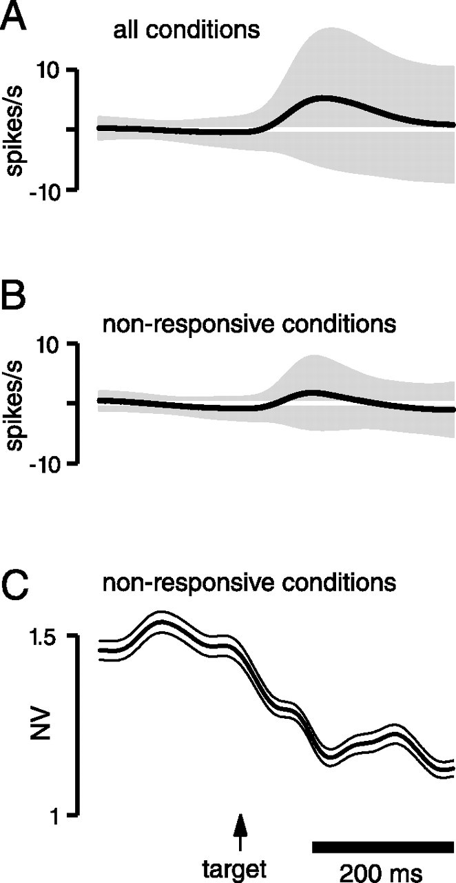
Reanalysis of the data in Figure 6A, restricting analysis to target locations that evoked little response. A, Change in mean firing rate (from baseline) as a function of time for all isolations and target locations (black trace; same as in Fig. 6A). The envelope plots the SD of the mean, across all isolations/target locations. Note that this reflects an entirely different kind of variability (variability across isolations and targets) than that reflected by the NV (variability across trials for a given isolation/target). B, Same as in A but after restricting the analysis to isolation/target location combinations with small changes in firing rate after target onset. A given isolation/target location was excluded if there was a >3 spike/s difference in mean firing rate between the baseline and delay periods. Of 658 original combinations (47 isolations by 14 target locations), 366 were excluded. As intended, mean firing rate changed even less than in A, and the SD was much smaller (the width of the envelope is still sometimes >3 spikes/s because that criterion was applied to firing rate averaged across the delay). C, The NV ± SE, computed after restricting the analysis to isolations/conditions with little change in firing rate, as described above. Compare with Figure 6A.

The above analysis indicates that the decline in variability is present even when mean firing rates change little. However, this analysis has the possible drawback that it preferentially excludes the contributions of the most active neurons (which may explain the modest decrease in effect size, if the most involved neurons are being excluded from the analysis). We therefore repeated the analysis using slightly different methodology. For each cell, we computed the median absolute change in firing rate, after target onset, for each condition. We then analyzed data separately for those conditions with absolute changes greater than the median (more responsive conditions) and less than the median (less responsive conditions). This ensured that each isolation contributed to both analyses. For two datasets (monkey G and the second from monkey B), the decline in the NV was slightly more pronounced for the more responsive conditions. For the other two datasets (monkey A and the first from monkey B), the decline was more pronounced for the less responsive conditions. Averaged across the four datasets, the decline in the NV (measured from 200 ms before until 200 ms after target onset) was remarkably similar for the more and less responsive conditions: 14 and 15%, respectively. Thus, the change in the NV is not strongly linked to the change in mean firing rate.

As a side note, it is reasonable to ask, for those conditions in which there was little change in firing rate, whether the variance still drops when expressed in raw un-normalized form. Supplemental Figure 2B (available at www.jneurosci.org as supplemental material) plots the mean un-normalized variance for the same data as in Figure 8C and makes two points. First, the effect can be seen even in the un-normalized variance. Second, even small changes in mean rate act to “corrupt” the un-normalized measurement. Supplemental Figure 2C (available at www.jneurosci.org as supplemental material) shows how the impact of mean rate on variability can be (approximately) factored out without normalizing, using a subtractive correction instead. Results are much the same as when using the divisive correction.

In summary, one cannot conclude that the NV measurement is entirely uncontaminated by changes in spike rate and the consequential changes in intrinsic spiking statistics. The relationship between mean spike rate and intrinsic spiking variability is presumably only approximately linear, so some “contamination” is likely inevitable. Still, changes in mean firing rate cannot be the primary cause of the decline in the NV after target onset, nor does that decline result somehow from divisive normalization. A more likely explanation for the drop in the NV is that the underlying firing rate, considered across trials, is becoming more consistent as the trial progresses. This suggests that, even for nonresponsive conditions, most neurons are changing their firing rate on most trials, something that is hidden in the mean firing rate.

Controls: changes in firing rate covariance

Another possibility is that the decline in the NV might result from more regular intrinsic spiking caused by some unknown network mechanism, perhaps the locking of spiking to a central rhythm. Although it would be difficult to entirely reject such a general hypothesis, the specific possibility that spikes lock to a central rhythm can be tested. If so, the magnitude of the covariance among neurons should increase during the delay, as they come to share a rhythm. To test this, we analyzed the change in spiking covariance (see Materials and Methods) for neural data recorded simultaneously using the implanted electrode array in monkey G. The covariance fell in parallel with the NV, dropping 66% by the time of the go cue (p < 10⁻⁵) (supplemental Fig. 3, available at www.jneurosci.org as supplemental material). Looking at the covariance before the movement (and with the data locked to the movement), the covariance was reduced by 92% (p < 10⁻⁶, relative to before target onset), reaching a minimum around the time of movement onset.

These findings argue against the possibility that the decline in the NV results from the locking (and subsequent regularization) of firing rates to a central rhythm. They also further address the broader issue (already considered above) of whether the decline might be attributable to changes in intrinsic spiking variability (e.g., more regular spike production) rather than an increasing consistency in the underlying firing rate across trials. A mathematical property of the covariance is that it is unaffected by the addition of independent noise to the two variables of interest. The covariance should therefore be uninfluenced by intrinsic spiking statistics, as long as they are independent between neurons. Thus, the finding that the covariance declines in parallel with the NV makes it very unlikely that the observed drop in variability results from a change in intrinsic spiking statistics. The change in the NV is most likely attributable to a decline in the across-trial variability of the underlying firing rate. As this variability declines, the covariance naturally declines as well. In this context, it is natural that the decline in the NV is more modest (∼35%) because it cannot fall below a certain “floor” value, limited by the intrinsic spiking variability. In contrast, the covariance could in principle fall to 0. Finally, we note that the covariance need not be (and was not) normalized and is dropping at a time when the un-normalized variance is rising along with mean firing rate (data not shown).

Time course of neural variability and the time course of motor preparation

The initial decline in the NV consumed 98–198 ms depending on the monkey and dataset. This is similar to the time course of the decline in RT with delay-period duration (∼100–200 ms) (Fig. 4). This is consistent with the idea that the magnitude of the NV indicates the approximate degree of motor preparation yet to be accomplished. Admittedly, this interpretation rests on some assumptions. First of all, it assumes that the increasing consistency of firing rates with time reflects their increasing accuracy (i.e., their increasing tendency to occupy the optimal subspace, whose boundaries cannot be easily inferred using current methods). Second, it assumes that there is a limit on the rate at which firing rates approach their putatively optimal values, such that progress before the go cue shortens the subsequent RT. The first assumption is difficult to test directly, although some indirect tests are possible (see below). The second assumption can be tested directly by comparing the rate of decline in the NV for trials with different delay durations. To do so, we used the dataset collected from monkey G using three discrete delay-period durations (30, 130, and 230 ms, randomly interleaved). Figure 9A shows the NV computed for the three delays, aligned to the onset of the go cue. The rate of decline in the NV is similar for the three delay durations. As a consequence, at the time of the go cue, the NV for the 230 ms delay has dropped to a plateau, whereas the NV for the 30 ms delay does not reach the same point until ∼80 ms later, potentially explaining why mean RT is longer. Figure 9C plots RT versus the NV at the time of the go cue for the three delays. The relationship increases monotonically. Thus, the height of the NV at the time of the go cue is predictive of RT, as would be expected if it reflected the average degree of motor preparation yet to be accomplished.

In contrast, Figure 9B shows that there was no simple relationship between RT and mean firing rate at the time of the go cue. This was true whether we considered all conditions (black) or just preferred conditions (gray). Note that this would also have been true had we considered firing rate at some fixed time (e.g., 100 ms) after the go cue. At that point, the 30 ms delay (which produced the longest RTs) produced the highest firing rates (Fig. 9A, top). At no time after the go cue were firing rates highest for the 230 ms delay duration, although it produced the shortest RT.

Caveats in relating the time course of the NV to the time course of motor preparation

Even if one were to fully accept the premise of the optimal-subspace hypothesis (that firing rates approach their “appropriate” values over time and that the resulting increase in consistency is reflected in the NV), there are still important caveats in attempting to relate the precise time course of the NV with the time course of motor preparation. As mentioned above, increasing consistency may imperfectly reflect increasing accuracy. More pragmatically, the manner in which the NV is computed is expected to introduce some distortions into the measurement of variability. For example, the measurement of the NV requires first filtering spike trains. To what degree does such filtering impact the observed time course of variability? Supplemental Figure 4 (available at www.jneurosci.org as supplemental material) plots the NV, computed using a variety of filters. The NV computed using a 15 ms (SD) Gaussian filter showed a similar time course to that computed using the 30 ms Gaussian (the standard length we used in our analyses). In particular, the time course of the initial decline is shortened only slightly when using the shorter filter: the NV still reaches a plateau at >100 ms after target onset. The decline after the go cue is also not obviously sharper for the 15 ms filter. On a more general note, there is nothing in the use of a Gaussian filter in particular that could create the overall effect. Results were similar when a box filter (±30 ms) was used (supplemental Fig. 4C, available at www.jneurosci.org as supplemental material). This computation (the NV with a box filter) is identical to computing the more standard Fano factor. We chose to use a Gaussian filter simply because it more effectively smoothes the spike trains. However, there is a possible drawback to the use of a Gaussian filter. The Fano factor has the advantage that it will always be unity for a Poisson process, even a nonhomogenous (time-varying) Poisson process, as long as the underlying firing rate is the same on every trial. This is not strictly true for the NV when computed with a Gaussian filter, which can show some transient departures from unity after sharp changes in firing rate (simulations not shown). However, transient departures from “ideal” behavior are expected to be small under most circumstances. Furthermore, the similarity of the results for the NV (supplemental Fig. 4A,B, available at www.jneurosci.org as supplemental material) and the Fano factor (supplemental Fig. 4 C,D, available at www.jneurosci.org as supplemental material) indicate that this is not a concern for the present dataset. More generally, there are inevitable tradeoffs when measuring across-trial variability. Longer filters (and smoother filters such as a Gaussian) better isolate signal from noise but at the expense of possibly distorting the time course. In summary, the observed time course of the NV will, in general, be influenced by the choice of filter. However, in the present case, the observed time course is not simply a consequence of filtering and is similar across a range of reasonable filters.

Relationship of neural variability to natural RT variability

The results above indicate that firing rates become more consistent after target onset. We chose to look for this increase in consistency because we suspected it might reflect an increase in accuracy: an increase in the average occupancy of an optimal subspace of firing rates. This hypothesis makes the following prediction, illustrated in Figure 10A. For some trials, the configuration of firing rates around the time of the go cue will lie within the optimal subspace (green dots, motor preparation is complete) and RTs will be short. For other trials, the configuration of firing rates will lie outside the optimal subspace (red dots, motor preparation is “sloppy” or incomplete) and RTs will be longer. Because of both a lack of adequate theory regarding the “representation” in PMd and the difficulty of making sufficiently detailed and extensive measurement of the tuning properties of individual neurons, it is not currently possible to estimate the location or extent of the optimal subspace with any degree of confidence. Nevertheless, we can exploit the fact that the variability of firing rates, as indexed by the NV, is expected to be greater for the long RT trials. This is perhaps the most striking prediction of the optimal-subspace hypothesis: that neural variability before the go cue ought to predict behavior after the go cue. Importantly, such a connection should be detectible (given sufficient data) without needing to know the “representational scheme” used by PMd, as long as we can assume that neural activity is on average nearly optimal.

Figure 10B plots the NV, around the time of the go cue, for trials with RTs longer than the median (red, long RT trials) and shorter than the median (green, short RT trials). For statistical power, we collapsed data across all seven datasets from monkey G (36–60 isolations per day, yielding 174,725 total neuron trials; data collapsed after segregating long vs short RTs within each dataset). Consistent with the above prediction, short RT trials had less variability in firing rate around the time of the go cue. The black trace at the bottom plots the mean percentage difference in the NV. This was computed by taking the percentage difference between the NV for the short and long RT trials for each isolation/condition and then computing the mean and SE.

The results of this analysis are summarized in Figure 10C (black symbols). Similar results were obtained for monkeys A and B, although the results are noticeably noisier given the smaller quantity of data (60 and 51 single-unit isolations, yielding 16,376 and 20,283 neuron trials, respectively). Before target onset (“pre-targ”), no monkey showed a significant difference in the NV for short and long RT trials (filled symbols indicate significance). During the delay (“delay”), variability was, for all monkeys, significantly lower for short RT trials. The same was true for the 200 ms interval after the go cue (“post-go”). For two of the three monkeys, there was less difference when measurements were made during the 200 ms period before, and locked to, movement onset (“pre-move”).

We also compared the difference in mean firing rate, across all neurons and conditions, for long and short RT trials. The blue trace in Figure 10B plots this difference as a function of time for monkey G. The difference is small and negative; RTs were shorter when firing rates were lower (p < 0.05 for the delay period, t test). However, for monkeys A and B, delay-period firing rates were on average slightly higher (1.4 and 0.8%) before short RTs (not significant, p > 0.05). Thus, the observed effects were both small and inconsistent across animals.

The tendency for short RT trials to have less variability around their mean also held for trials with a negligible (30 ms) delay period. Figure 10D plots the NV for trials with RTs shorter and longer than the median. Data are from 2 d of experiments using monkey G. The NV drops more rapidly for short RT trials. The difference (black trace) was significant, both at individual time points (90–170 ms after the go cue; maximum difference was 5.3%; p < 0.01) and when averaged over the 200 ms period after go cue (2.5%; p < 0.05). When measured over the 200 ms premovement period, locked to movement onset, the difference in the NV disappeared or even reversed slightly, being 1.4% (p > 0.05) in the direction of a higher NV before shorter RTs. Thus, in three of the four cases, the difference in the NV between short and long RT trials was reduced or eliminated during the premovement period with data locked to movement onset. This is consistent with the idea that the degree of firing-rate accuracy reached by the time of movement onset is similar for long and short RT trials.

For these 30 ms delay-period trials, we also examined the difference in mean firing rate between long and short RT trials (Fig. 10D, blue trace). For the 200 ms post-go-cue period, the difference was not significantly different from 0 (0.4%; p = 0.8). The difference in mean firing rate did become significant by the end of this interval (maximum of 4.8%; p < 0.01, measured 190 ms after the go cue), although by this time movement-related activity is present, especially for trials with shorter RTs. Thus, this difference is more likely a result of, rather than a cause of, the difference in RTs. Interpretational difficulties related to the overlap of preparatory and movement-related activity are difficult to entirely overcome with this experimental design using a very short delay. Nevertheless, we include these data to illustrate that the principal effect of these analyses (a lower NV before shorter RTs) is not somehow an artifact of longer instructed delays.

For both the long and short delays (Fig. 10B–D), the RT-dependent difference in variability is rather small in absolute terms (∼5%). However, it is worth noting that there is probably a floor below which the NV cannot drop because of the intrinsic variability of spike production (e.g., for Poisson spiking statistics, the floor would be at unity). Thus, 5% in absolute terms could easily be much higher in terms of true across-trial variability present at that time.

RTs are shortest when firing rates are near their mean

The above results indicate that RTs are shortest not when overall firing rates are highest but when variability is lowest: in other words, when firing rates are closest to their mean. This effect can be observed more directly, and on a trial-by-trial basis, by exploiting the large dataset collected across days from monkey G. Figure 11 plots, for each trial and isolation, RT versus delay-period firing rate relative to the mean for that isolation and target location. It is essentially impossible to glean anything by direct visual inspection of the cloud of 174,725 data points. This is not surprising: most of the measured variability in firing rate is presumably attributable to intrinsic spiking variability, which is not expected to predict RT. To look for an underlying relationship, we used regression to obtain the coefficients of a quadratic equation: RT = c₀ + c₁ × FR + c₂ × FR² (curved trace), where FR is firing rate. The explained variability is low (R² = 0.0008), as expected given the above assumption that most variability is intrinsic. Yet the fit was nevertheless statistically significant (p < 10⁻¹⁰) and revealing of a simple pattern: RTs became longer as firing rates departed from their mean in either direction. This analysis has some disadvantages relative to the NV analysis: it cannot reveal the first principal finding (the decline in variability over time), nor does it track the time course of the relationship between variability and RT. Nevertheless, it provides an alternate way of observing the second principal finding: RTs are shortest not when firing rates are highest but when firing rates are somewhere near their mean.

Is it possible that RT outliers dominated the analyses in Figures 10 and 11? Perhaps there were a handful of trials in which the monkey was distracted, resulting in very long RTs and firing rates dramatically different from the mean. We repeated the analyses in Figures 10B and 11 using only trials with RTs between 200 and 300 ms (the heart of the natural distribution). Results were essentially identical to those initially obtained. A second possible concern is that the analyses in Figures 10 and 11 collapse across trials with different delay durations. Might the observed effects be attributable simply to parallel changes, as the delay passes, in RT and neural variability? A priori, this is probably a minor concern because all data are from trials with delay durations >200 ms, after which RTs and the NV are fairly stable. Empirically, we found that effects were just as strong (for both analyses) when we considered only trials with a 230 ms delay period (data coming from the two datasets in which we used three discrete delay durations).

“Tuning” of the changes in variability

We showed above that the decline in the NV could be observed even when the mean rate changed little (Fig. 8 and accompanying analyses). Those analyses provided an important control but did not systematically examine the NV as a function of target direction. In particular, are the changes in the NV larger or smaller for targets in the preferred direction of a neuron? It is unclear what to expect. In its simplest form, the optimal-subspace hypothesis suggests that variability should decline approximately equally for all targets. Conversely, some tuning would not be surprising because the dimensions in which variability is “acceptable” could vary depending on the movement being planned. To examine this issue, we computed both mean firing rate and the NV as a function of target location relative to the preferred direction (see Materials and Methods). This analysis was performed for monkeys G and A, as the task involved all target directions, but not for monkey B, in which most neurons were tested using only two target directions. The gray symbols in Figure 12 show the mean firing rate, averaged across all neurons. Data for each neuron were rotated so that the preferred direction is to the right, with more clockwise points corresponding to more clockwise target directions. For both monkeys, firing rates are (by definition) higher in the preferred direction. Monkey G (Fig. 12A) exhibited (on average) inhibition below baseline (gray circle) for the anti-preferred directions, whereas monkey A (Fig. 12B) exhibited (on average) some excitation even for the anti-preferred directions (6 spikes/s relative to baseline vs 12 spikes/s in the preferred direction). This pattern does not reflect a lack of direction tuning in this dataset: the majority of neurons showed a significant effect of direction, which could be quite large when measured using the preferred distance and instructed speed, but rather the fact that many neurons showed positive responses for all conditions (perhaps a consequence of bias when isolating single units with a moveable electrode).

Figure 12.

Analysis, for monkeys G and A (A, B) of the firing rate (gray symbols) and the NV (black symbols) as a function of target direction relative to the preferred. Each point is averaged across all neurons and all targets (distances, and for monkey A, instructed speeds) in that direction. Data from each neuron are aligned so that the preferred target direction (PD) is to the right, with more clockwise points corresponding to the more clockwise target directions. Circles give the baseline NV (outer black rings, ±1 SE on either side of the mean) and the average baseline firing rate (inner gray ring) measured before target onset. For scale, the baseline firing rate was 10 and 14 spikes/s for the two monkeys. The baseline NV was 1.44 and 1.31. The SE of the NV is shown for individual data points when larger than the symbol size.

The black traces in Figure 12 plot the NV at the time of the go cue. For all target directions and for both monkeys, the mean NV at the time of the go cue was reduced relative to baseline (outer circle, measured 200 ms before target onset). Only modest tuning of the NV was observed. For monkey G (A), the NV was most reduced (to 1.03 ± 0.04 from a baseline of 1.44 ± 0.02) for targets in the preferred direction and less reduced (to 1.18 ± 0.05 and 1.12 ± 0.04) for the directions most opposite the preferred. For monkey A (B) the opposite pattern was observed. The NV was slightly less reduced (to 1.14 ± 0.06 from a baseline of 1.31 ± 0.04) for the preferred direction relative to the most opposite directions (0.97 ± 0.06 and 1.08 ± 0.06).

Caution should be used in interpreting the modest tuning of the NV and not only because results were different for the two monkeys. By design, this analysis compares the NV across conditions with very different mean firing rates. It is unlikely that normalization perfectly factors out the contribution of intrinsic variability and its relationship with mean rate. A related issue is that the normalization used in computing the NV also acts to normalize any true across-variability. Thus, one must be concerned that weak tuning might depend on exactly how one attempts to factor out the contribution of intrinsic variability. This was indeed the case. For example, we recomputed the analysis in Figure 12A using the variance minus 0.7 times the mean (after first scaling the mean by k) (supplemental Fig. 2C, available at www.jneurosci.org as supplemental material). This method makes the (not implausible) approximation that intrinsic variability has a variance that scales linearly with the mean but with a slope slightly less than expected from a Poisson process. In that analysis, the overall decline in variability was still quite evident, but the observed tuning was essentially gone (i.e., the preferred and anti-preferred directions showed similar declines). Thus, the basic effect is robust across reasonable assumptions regarding the relationship of intrinsic variability to mean rate, but the modest tuning is not. Of course, it is possible that individual neurons did show strong tuning of the NV but that there was not, across the population, a consistent relationship between that tuning and the tuning of the mean firing rate. A lack of statistical power precludes any straightforward investigation of this possibility.

Discussion

Time course of neural variability

The NV reveals a previously unknown degree of temporal structure in the variability of neural activity during a delayed reach task. Variability declines rather dramatically after target onset and more modestly after the go cue. Because the NV is a measurement of across-trial firing-rate variability, the most natural interpretation is that there is a decline in the across-trial variability of the underlying firing rates. Alternately, the decline in the NV might reflect a change in the within-trial cell-intrinsic process of spike production (e.g., from cortex-like statistics to vestibular-afferent-like statistics). A number of controls exclude the most obvious ways this might happen (most trivially, with increasing firing rate), but it is difficult to completely exclude this possibility given extracellular recordings alone. Still, the proposal that cell-intrinsic spiking statistics change would be quite radical. In contrast, it is quite natural to suppose that the underlying firing rate of a neuron may vary across trials and that the degree of variability might change with time. Under this interpretation, it is unsurprising that firing rates can become more consistent (across trials) even when the mean rate (across trials) changes little. A neuron that changes its rate little on average may nevertheless be changing its firing rate rather a lot on most individual trials.

A decrease in response variability during driven activity has been reported previously in a variety of contexts (Werner and Mountcastle, 1963; Sestokas and Lehmkuhle, 1988; Bair and Koch, 1996; de Ruyter van Steveninck et al., 1997; Buracas et al., 1998). However, the interpretation of such effects (and even what is meant by variability) has differed. To our knowledge, the current study is the first to demonstrate, in cortex, a stimulus-driven decline in across-trial variability that is unambiguously not attributable to changes in mean rate. Still, this type of effect is not necessarily surprising: previous work has argued that much of the observed variability in cortex is a network property (Arieli et al., 1996; Buracas et al., 1998), which might naturally be expected to change with task demands.

Relationship between firing rates and RT

We found that RTs are shortest when variability is lowest: when firing rates are closest to their mean. This was true when comparing RTs produced by different delay durations (Fig. 9) and for natural RT variability (Figs. 10, 11). We did not find a consistent relationship between higher firing rates and shorter RTs, across either delay durations or the natural variability. This contrasts with Riehle and Requin (1993) and Bastian et al. (2003), who found negative correlations between firing rate and RT. However, it should be stressed that neither our results nor the optimal-subspace hypothesis conflict with the finding that, under some circumstances, higher firing rates are associated with shorter RTs. Exactly this result is expected if firing rates tend to “undershoot” the optimal subspace. Previous studies often used long (1–2 s) delay periods and generous RT limits, providing little incentive for consistent preparation during the delay. Motor preparation may have been present on some trials (leading to higher firing rates and shorter RTs) and absent on others (leading to lower firing rates and longer RTs).

Although our results do not necessarily conflict with previous experimental findings, they certainly do conflict with the rise-to-threshold hypothesis that was motivated by those findings. That hypothesis predicts a consistent relationship between higher firing rates and shorter RTs, something we did not observe. Previous work has also sometimes failed to find such a relationship. In addition to the study by Crammond and Kalaska (2000) discussed in Introduction, we note that Lecas et al. (1986) found both negative and positive correlations: of 82 neurons excited during the delay period, 10 showed a negative correlation with RT (consistent with a threshold mechanism), whereas five showed a positive correlation (inconsistent with a threshold mechanism).

Interpretation in the context of the optimal-subspace hypothesis

If a movement is in whole or in part a consequence of the preparatory activity present at the time it is triggered, then it would seem critical that such activity be optimized before triggering. We hypothesize that such optimization is the behaviorally inferred process of motor preparation. Our experiments and analyses were designed to test two central predictions of this hypothesis. First, if the brain is actively “trying” to bring firing rates to a particular state, then this should produce a decline in variability. The time course of that decline should approximately mirror the changes in RT that occur as motor preparation progresses. Second, if the brain can sense when preparatory activity is accurate and if activity is on average approximately accurate, then RTs should be shortest when variability is low, i.e., when firing rates are closest to their mean (we are not suggesting that the brain cares about variability per se but rather that reduced variability is a correlate of increased accuracy). That these two predictions were born out lends support to the optimal-subspace hypothesis. Clearly, however, additional experiments are both needed and possible. Along these lines, we reported recently that disruption of PMd activity, around the time of the go cue, increases RT (Shenoy and Churchland, 2004) and that variability in the state of preparatory activity predicts variability in reach speed (Churchland and Shenoy, 2004).

The optimal-subspace hypothesis contrasts with the rise-to-threshold hypothesis, which has been either explicit (Erlhagen and Schoner, 2002) or implicit in many studies of reach preparation. The rise-to-threshold hypothesis is almost a special case of the optimal-subspace hypothesis (with the entire region above threshold being optimal). However, for the optimal-subspace hypothesis, bringing the firing-rate vector within the optimal-subspace is merely permissive: the movement is ready to be triggered when appropriate. In contrast, the rise-to-threshold hypothesis holds that it is the crossing of threshold that actually triggers the movement. Finally, the rise-to-threshold hypothesis makes assumptions about the nature of the representation, in particular that an overall increase in firing rates will code for the same movement but with greater commitment, that are not made by the optimal-subspace hypothesis.

The lack of a consistent relationship between higher firing rates and shorter RTs conflicts with the basic rise-to-threshold hypothesis but does not necessarily rule out more elaborate versions. Perhaps the trigger is applied not to total or peak firing rate but to some more complicated function of firing rate across the population. Still, the observed changes in neural variability (and the relationship with RT) are not straightforward predictions of the rise-to-threshold hypothesis. That hypothesis does predict a decline in variability before movement onset, if analysis is locked to movement onset (so that the threshold crossing occurs at a similar time in every trial). However, if one assumes a variable rate of rise (typical for such models), the rise-to-threshold hypothesis predicts a rise (rather than a decline) in across-trial variability after target onset.

Tracking the time course of cortical processing

Measurements of variability have been extensively used in the analysis of neural data (Tolhurst et al., 1983; Gur et al., 1997; Bair and O'Keefe, 1998; Averbeck and Lee, 2003). Yet the present study is, to our knowledge, the first to use a measurement of variability in an attempt to track the time course of internal processing (although this approach was anticipated by Horwitz and Newsome, 2001). Given present results, it seems plausible that the measured increase in consistency reflects an increase in accuracy, an increasing likelihood that firing rates have reached their appropriate values. This highlights an advantage of measuring firing rate variability. Even when little is known regarding the representation used by an area of interest (so that the experimenter cannot know which firing-rate vectors count as accurate or appropriate), an index of variability can potentially allow one to infer the time course with which firing rates become accurate. Clearly, there are caveats to this approach. Still, given the number of brain areas in which the representation or “coordinate frame” is unclear, such a method would seem useful.

On-line and off-line motor control

For all but the briefest movements, on-line motor control (i.e., control during the movement) involves feedback based on sensory signals. It has been proposed that a “forward model” could also provide signals for feedback control (Kawato et al., 1987; Wolpert et al., 1995; Kawato, 1999), predicting the consequences of motor commands and allowing for rapid optimization of the control signals being sent to the periphery. In principle, a forward model could be used even before movement begins (Hirayama et al., 1993; Wada and Kawato, 1993). By predicting the consequences of the current motor plan, a forward model could allow that plan to be optimized before executing the movement. Crucially, the forward model would be able to predict when a given motor plan is likely to be inaccurate and allow the brain to delay movement until inaccuracies are corrected. Thus, the optimal-subspace hypothesis presented above can be readily reconceived using concepts already used in the computational study of motor control. One need only suppose that already familiar mechanisms (e.g., feedback control using a forward model) are operative not only during movement but during movement preparation as well.

References

- Arieli A, Sterkin A, Grinvald A, Aertsen A (1996). Dynamics of ongoing activity: explanation of the large variability in evoked cortical responses. Science 273:1868–1871. [DOI] [PubMed] [Google Scholar]
- Averbeck BB, Lee D (2003). Neural noise and movement-related codes in the macaque supplementary motor area. J Neurosci 23:7630–7641. [DOI] [PMC free article] [PubMed] [Google Scholar]
- Bair W, Koch C (1996). Temporal precision of spike trains in extrastriate cortex of the behaving macaque monkey. Neural Comput 8:1185–1202. [DOI] [PubMed] [Google Scholar]
- Bair W, O'Keefe LP (1998). The influence of fixational eye movements on the response of neurons in area MT of the macaque. Vis Neurosci 15:779–786. [DOI] [PubMed] [Google Scholar]
- Bastian A, Riehle A, Erlhagen W, Schoner G (1998). Prior information preshapes the population representation of movement direction in motor cortex. NeuroReport 9:315–319. [DOI] [PubMed] [Google Scholar]
- Bastian A, Schoner G, Riehle A (2003). Preshaping and continuous evolution of motor cortical representations during movement preparation. Eur J Neurosci 18:2047–2058. [DOI] [PubMed] [Google Scholar]
- Batista A, Yu B, Santhanam G, Ryu SI, Shenoy KV (2004). Coordinate frames for reaching in macaque dorsal premotor cortex (PMd). Soc Neurosci Abstr 30:191.197. [Google Scholar]
- Batista AP, Santhanam G, Yu BM, Ryu SI, Afshar A, Shenoy KV (2005). Heterogeneous coordinate frames for reaching in macaque PMd. Soc Neurosci Abstr 31:363.312. [Google Scholar]
- Berry MJ II, Meister M (1998). Refractoriness and neural precision. J Neurosci 18:2200–2211. [DOI] [PMC free article] [PubMed] [Google Scholar]
- Boussaoud D (1995). Primate premotor cortex: modulation of preparatory neuronal activity by gaze angle. J Neurophysiol 73:886–890. [DOI] [PubMed] [Google Scholar]
- Buracas GT, Zador AM, DeWeese MR, Albright TD (1998). Efficient discrimination of temporal patterns by motion-sensitive neurons in primate visual cortex. Neuron 20:959–969. [DOI] [PubMed] [Google Scholar]
- Carandini M (2004). Amplification of trial-to-trial response variability by neurons in visual cortex. PLoS Biol 2:E264. [DOI] [PMC free article] [PubMed] [Google Scholar]
- Carpenter RH, Williams ML (1995). Neural computation of log likelihood in control of saccadic eye movements. Nature 377:59–62. [DOI] [PubMed] [Google Scholar]
- Churchland MM, Shenoy KV (2004). Trial-by-trial movement variability is predicted by recorded plan activity Presented at the 14th Annual Meeting of the Neural Control of Movement Society, Sitges, Spain, March.
- Churchland MM, Yu B, Ryu SI, Santhanam G, Shenoy KV (2004). Reaction time and the time-course of cortical pre-motor processing. Soc Neurosci Abstr 30:603.5. [Google Scholar]
- Cisek P, Kalaska JF (2002). Modest gaze-related discharge modulation in monkey dorsal premotor cortex during a reaching task performed with free fixation. J Neurophysiol 88:1064–1072. [DOI] [PubMed] [Google Scholar]
- Crammond DJ, Kalaska JF (2000). Prior information in motor and premotor cortex: activity during the delay period and effect on pre-movement activity. J Neurophysiol 84:986–1005. [DOI] [PubMed] [Google Scholar]
- Day BL, Rothwell JC, Thompson PD, Maertens de Noordhout A, Nakashima K, Shannon K, Marsden CD (1989). Delay in the execution of voluntary movement by electrical or magnetic brain stimulation in intact man. Evidence for the storage of motor programs in the brain. Brain 112:649–663. [DOI] [PubMed] [Google Scholar]
- de Ruyter van Steveninck RR, Lewen GD, Strong SP, Koberle R, Bialek W (1997). Reproducibility and variability in neural spike trains. Science 275:1805–1808. [DOI] [PubMed] [Google Scholar]
- Erlhagen W, Schoner G (2002). Dynamic field theory of movement preparation. Psychol Rev 109:545–572. [DOI] [PubMed] [Google Scholar]
- Georgopoulos AP, Kalaska JF, Caminiti R, Massey JT (1982). On the relations between the direction of two-dimensional arm movements and cell discharge in primate motor cortex. J Neurosci 2:1527–1537. [DOI] [PMC free article] [PubMed] [Google Scholar]
- Ghez C, Favilla M, Ghilardi MF, Gordon J, Bermejo R, Pullman S (1997). Discrete and continuous planning of hand movements and isometric force trajectories. Exp Brain Res 115:217–233. [DOI] [PubMed] [Google Scholar]
- Godschalk M, Lemon RN, Kuypers HG, van der Steen J (1985). The involvement of monkey premotor cortex neurones in preparation of visually cued arm movements. Behav Brain Res 18:143–157. [DOI] [PubMed] [Google Scholar]
- Gur M, Beylin A, Snodderly DM (1997). Response variability of neurons in primary visual cortex (V1) of alert monkeys. J Neurosci 17:2914–2920. [DOI] [PMC free article] [PubMed] [Google Scholar]
- Hanes DP, Schall JD (1996). Neural control of voluntary movement initiation. Science 274:427–430. [DOI] [PubMed] [Google Scholar]
- Hirayama M, Kawato M, Jordan MI (1993). The cascade neural network model and a speed-accuracy trade-off of arm movement. J Mot Behav 25:162–174. [DOI] [PubMed] [Google Scholar]
- Horwitz GD, Newsome WT (2001). Target selection for saccadic eye movements: direction-selective visual responses in the superior colliculus. J Neurophysiol 86:2527–2542. [DOI] [PubMed] [Google Scholar]
- Kawato M (1999). Internal models for motor control and trajectory planning. Curr Opin Neurobiol 9:718–727. [DOI] [PubMed] [Google Scholar]
- Kawato M, Furukawa K, Suzuki R (1987). A hierarchical neural-network model for control and learning of voluntary movement. Biol Cybern 57:169–185. [DOI] [PubMed] [Google Scholar]
- Keele SW (1968). Movement control in skilled motor performance. Psychol Bull 70:387–403. [Google Scholar]
- Kurata K (1989). Distribution of neurons with set- and movement-related activity before hand and foot movements in the premotor cortex of rhesus monkeys. Exp Brain Res 77:245–256. [DOI] [PubMed] [Google Scholar]
- Kutas M, Donchin E (1974). Studies of squeezing: handedness, responding hand, response force, and asymmetry of readiness potential. Science 186:545–548. [DOI] [PubMed] [Google Scholar]
- Lecas JC, Requin J, Anger C, Vitton N (1986). Changes in neuronal activity of the monkey precentral cortex during preparation for movement. J Neurophysiol 56:1680–1702. [DOI] [PubMed] [Google Scholar]
- Oram MW, Hatsopoulos NG, Richmond BJ Donoghue JP (2001). Excess synchrony in motor cortical neurons provides redundant direction information with that from coarse temporal measures. J Neurophysiol 86:1700–1716. [DOI] [PubMed] [Google Scholar]
- Osborne LC, Bialek W, Lisberger SG (2004). Time course of information about motion direction in visual area MT of macaque monkeys. J Neurosci 24:3210–3222. [DOI] [PMC free article] [PubMed] [Google Scholar]
- Padoa-Schioppa C, Li CS, Bizzi E (2002). Neuronal correlates of kinematics-to-dynamics transformation in the supplementary motor area. Neuron 36:751–765. [DOI] [PubMed] [Google Scholar]
- Riehle A, Requin J (1989). Monkey primary motor and premotor cortex: single-cell activity related to prior information about direction and extent of an intended movement. J Neurophysiol 61:534–549. [DOI] [PubMed] [Google Scholar]
- Riehle A, Requin J (1993). The predictive value for performance speed of preparatory changes in neuronal activity of the monkey motor and premotor cortex. Behav Brain Res 53:35–49. [DOI] [PubMed] [Google Scholar]
- Riehle A, MacKay WA, Requin J (1994). Are extent and force independent movement parameters? Preparation- and movement-related neuronal activity in the monkey cortex. Exp Brain Res 99:56–74. [DOI] [PubMed] [Google Scholar]
- Roitman JD, Shadlen MN (2002). Response of neurons in the lateral intraparietal area during a combined visual discrimination reaction time task. J Neurosci 22:9475–9489. [DOI] [PMC free article] [PubMed] [Google Scholar]
- Rosenbaum DA (1980). Human movement initiation: specification of arm, direction, and extent. J Exp Psychol Gen 109:444–474. [DOI] [PubMed] [Google Scholar]
- Sestokas AK, Lehmkuhle S (1988). Response variability of X- and Y-cells in the dorsal lateral geniculate nucleus of the cat. J Neurophysiol 59:317–325. [DOI] [PubMed] [Google Scholar]
- Shenoy K, Churchland M (2004). Changes in reaction time induced by microstimulation in PMd. Soc Neurosci Abstr 30:603.6. [Google Scholar]
- Snyder LH, Batista AP, Andersen RA (1997). Coding of intention in the posterior parietal cortex. Nature 386:167–170. [DOI] [PubMed] [Google Scholar]
- Tanji J, Evarts EV (1976). Anticipatory activity of motor cortex neurons in relation to direction of an intended movement. J Neurophysiol 39:1062–1068. [DOI] [PubMed] [Google Scholar]
- Tolhurst DJ, Movshon JA, Dean AF (1983). The statistical reliability of signals in single neurons in cat and monkey visual cortex. Vision Res 23:775–785. [DOI] [PubMed] [Google Scholar]
- Wada Y, Kawato M (1993). A neural network model for arm trajectory formation using forward and inverse dynamics models. Neural Netw 6:919–932. [Google Scholar]
- Weinrich M, Wise SP (1982). The premotor cortex of the monkey. J Neurosci 2:1329–1345. [DOI] [PMC free article] [PubMed] [Google Scholar]
- Weinrich M, Wise SP, Mauritz KH (1984). A neurophysiological study of the premotor cortex in the rhesus monkey. Brain 107:385–414. [DOI] [PubMed] [Google Scholar]
- Werner G, Mountcastle VB (1963). The variability Of central neural activity in a sensory system, and its implications for the central reflection of sensory events. J Neurophysiol 26:958–977. [DOI] [PubMed] [Google Scholar]
- Wise SP (1985). The primate premotor cortex: past, present, and preparatory. Annu Rev Neurosci 8:1–19. [DOI] [PubMed] [Google Scholar]
- Wolpert DM, Ghahramani Z, Jordan MI (1995). An internal model for sensorimotor integration. Science 269:1880–1882. [DOI] [PubMed] [Google Scholar]