Auditory Midbrain and Nerve Responses to Sinusoidal Variations in Interaural Correlation

Abstract

The human sensitivity to interaural temporal differences in the acoustic waveforms to the two ears shows remarkable acuity but is also very sluggish. Fast changes in binaural parameters are not detectable, and this inability contrasts sharply with the excellent temporal resolution of the monaural auditory system. We studied the response of binaural neurons in the inferior colliculus of the cat to sinusoidal changes in the interaural correlation of broadband noise. Responses to the same waveforms were also obtained from auditory nerve fibers and further analyzed with a coincidence analysis. Overall, the auditory nerve and inferior colliculus showed a similar ability to code changes in interaural correlation. This ability extended to modulation frequencies an order of magnitude higher than the highest frequencies detected binaurally in humans. We conclude that binaural sluggishness is not caused by a lack of temporal encoding of fast binaural changes at the level of the midbrain. We hypothesize that there is no neural substrate at the level of the midbrain or higher to read out this temporal code and that this constitutes a low-pass “sluggishness” filter.

Introduction

Stereo-based spatial hearing and visual depth perception share many similarities. Behaviorally, both systems show temporal sluggishness. Temporal resolution for the modulation of binocular disparities is lower than for contrast modulation. The limit is thought to reside in the cross-correlation-type operation performed in primary visual cortex on monocular inputs that are temporally bandpass (Nienborg et al., 2005). In hearing, temporal resolution is much lower for binaural disparities than for monaural amplitude modulation (AM) [“binaural sluggishness” (Grantham and Wightman, 1978; Grantham, 1982)]. Its physiological source is unknown.

Different psychophysical paradigms have been used to quantify sluggishness (Kollmeier and Gilkey, 1990; Culling and Summerfield, 1998; Culling and Colburn, 2000; Bernstein et al., 2001; Boehnke et al., 2002). Two classic studies (Grantham and Wightman, 1978; Grantham, 1982) used a systems approach to estimate the binaural integration time, in which the basic stimulus consisted of noise bands with sinusoidally varying interaural correlation. Grantham (1982) varied the frequency and depth at which the interaural correlation was modulated and constructed binaural modulation transfer functions by plotting detection thresholds as a function of modulation frequency. The main conclusion was that the detectability of modulation in interaural correlation is limited to very low modulation frequencies: binaural integration times were estimated at ∼100 ms, with some evidence of a dependence on the center frequency of the noise band used. Although estimates of binaural integration times vary across studies, they consistently range from several tens to hundreds of milliseconds, which is in stark contrast to monaural integration times, which are only ∼2–3 ms (Rodenburg, 1977; Viemeister, 1979).

In contrast to vision, sluggishness cannot occur at the site of the initial stereo comparison. Neurons in the medial superior olive (MSO) are sensitive to interaural time differences (ITDs) (Goldberg and Brown, 1969) and need submillisecond resolution to perform the timing comparison of phase-locked signals up to a few kilohertz. However, sluggishness may first appear in projection targets of the MSO. The inferior colliculus (IC) is the major auditory structure in the midbrain in which integration of subcollicular targets occurs (Oliver, 2005), and the ability of its neurons to synchronize to or “follow” various temporal aspects of sounds is generally more limited than in peripheral neurons. For example, phase locking to pure or amplitude-modulated tones does not extend to frequencies as high as in subcollicular structures (Kuwada et al., 1984; Batra et al., 1989; Stanford et al., 1992; Krishna and Semple, 2000); fast changes in ITDs of tones, generated with binaural beats (BBs), are only followed up to 80 Hz (Yin and Kuwada, 1983); and sensitivity to dynamic changes in ITD, which may require temporal integration, arises at the level of the IC and is not present in the MSO (Spitzer and Semple, 1993, 1995). We therefore examined the ability of IC neurons to respond to dynamic changes in binaural parameters. In an approach similar to that of Grantham (1982), we measured binaural transfer functions but used a constant input rather than a constant output method.

Parts of this work have been published previously as a preliminary report (Joris, 1996).

Materials and Methods

Preparation. The general procedures are as described previously (Joris et al., 2005a). Experiments were performed at the Department of Physiology, University of Wisconsin–Madison, and the procedures were approved by the University of Wisconsin Animal Care Committee. Anesthesia was induced in young adult cats with an intramuscular mixture of acepromazine (0.2 mg/kg) and ketamine (20 mg/kg). Body temperature was maintained with a heating pad and rectal thermometer. An intravenous line was placed to deliver fluid and sodium pentobarbital so as to eliminate the withdrawal reflex to toe pinch. The trachea was cannulated, the external ear canals were exposed and cut, and fine polyethylene tubing (inner diameter, 0.9 mm; length, ∼30 cm) was glued to an opening in the bulla to prevented buildup of static pressure. The IC was exposed through a craniotomy and aspiration of occipital cortex. In some cases, part of the bony tentorium was removed to obtain better access to the IC. A chamber was cemented to the skull, which served as a support for a hydraulic microdrive with which tungsten or indium electrodes were advanced into the tissue. Warm agar was poured over the exposed IC after positioning of the electrode in an effort to stabilize the preparation.

Tight-fitting ear bars were inserted into the cut ear canals while visualizing the eardrums through the ear bars to ensure proper placement. A probe tube, coupled to a Brüel and Kjær (Nærum, Denmark) 12.7 mm condenser microphone, protruded from the ear bar and was used to measure the sound-pressure level (SPL) (decibels relative to 20 μPa) near the eardrum for tones from 100 to 65,000 Hz (in 50 Hz steps). The dynamic phones and ear bar/calibration probe assembly were as described previously (Chan et al., 1993). Stimuli were generated with a 16 bit, 524 kHz digital stimulus system (Olson et al., 1985). Precautions were taken to minimize acoustic crosstalk through the stimulus system (Gibson, 1982), and control experiments in the auditory nerve (AN) (see below) (Joris and Smith, 1998) confirmed the high level of acoustic isolation.

Recording. Standard procedures were followed to amplify and monitor the extracellular recording signal. Spikes times at 1 or 10 μs resolution were obtained through a two-level discriminator and unit event timer, interfaced to a Vaxstation 3200. Single units were studied in dorsoventrally and lateromedially directed penetrations. We focused on cells that showed sustained responses and ITD sensitivity to broadband noise and that were in the central nucleus of the IC as judged by the tonotopic progression and other physiological criteria. The brains were routinely processed histologically to confirm that the electrode tracks traversed the central nucleus. Lesions and detailed reconstructions were performed in selected cases to localize cells with binaural envelope sensitivity (Joris, 2003).

Basic response properties routinely tested were frequency tuning, binaural response type, and sensitivity to ITDs. The latter was assessed with a series of tones of ascending frequency containing a binaural beat (Kuwada et al., 1979) and with a broadband noise of which the ITD was varied: only cells whose response was clearly modulated at the beat frequency or was clearly dependent on ITDs of noise were further studied. Characteristic frequency (CF) and spontaneous rate were determined with a tuning curve tracking algorithm using binaural and/or monaural stimulation. A noise-delay curve, i.e., response rate as a function of ITD, was obtained for correlated, uncorrelated, and anticorrelated noise (these conditions are here indicated as A/A, A/B, and A/–A) with the following typical parameters (duration, repetition interval, and number of repetitions): 1/1.5 s for 20 times. The noise bandwidth varied between 4 and 32 kHz, depending on the CF of the cell studied. In eight cells for which CF was not available, we obtained the “dominant frequency” from noise-delay functions, as described by Joris et al. (2005a).

Stimuli and analysis. The basic stimulus of interest in this study (for a full description, see Grantham and Wightman, 1979, their Appendix) is a pair of noise waveforms of which the interaural correlation fluctuates at a frequency ω = 2π f_r: ρ(t) = sin ωt. Figure 1 illustrates the construction of the stimuli and the labeling shorthands used in this paper. Two noise tokens (“A” and “B”) were digitally created from two 32-kHz-wide noises (5 s, 320,000 points). Energy below 100 Hz and above 8000 Hz was removed with digital filtering. In some of the previous experiments, we used 16-kHz-wide noises (10 s), low-pass filtered at 4 kHz. Token A was multiplied by sinf_rt and token B by cosf_rt (f_r = 1 Hz in Fig. 1), and the two resulting waveforms (“Asin1” and “Bcos1”) were summed (“AB1”). This summed waveform was delivered to one ear and one of the original tokens to the other ear (A in Fig. 1, resulting in the pair “A/AB1”). Such a pair of binaural waveforms has an interaural correlation that varies sinusoidally between 1 and –1 at frequency f_r (Fig. 1, rightmost panel) and will be referred to as an oscillating correlation (OSCOR) stimulus. Several versions of these stimuli, obtained from different noise tokens, were calculated and stored on disk for the following f_r: 1, 2, 5, 10, 20, 50, 75, 100, 150, 200, 300, 400, 500, 750, and 1000 Hz. We express the noise sound level as “effective SPL,” which is the power in a one-third octave frequency band geometrically centered at the CF of the cell, averaged for the two ears, and expressed in decibels relative to 20 μPa. Effective SPL was calculated using the actual noise waveforms and calibration curves used during data collection.

Figure 1.

Construction of stimuli with oscillating interaural correlation (OSCOR stimuli). A and B indicate two independent, equal power noise tokens. Each token is multiplied by a sinusoidal or cosinusoidal modulator, at 1 Hz in the examples shown here, and the resulting waveforms (Asin1 and Bcos1) are summed (resulting in waveform AB1). The panel on the right shows interaural correlation between A and AB1, calculated with a sliding 1 ms rectangular time window. The interaural correlation varies between fully correlated (at 250 ms) and anticorrelated (at 750 ms).

Two important properties of the OSCOR stimulus may not immediately be obvious. First, there is no amplitude modulation in stimulus ABf_r (although there is in the constituent stimuli Asinf_r and Bcosf_r); second, the interaural correlation between A and ABf_r is modulated at f_r, but the Asinf_r and Bcosf_r waveforms are amplitude modulated at frequency 2f_r (Fig. 1) because there is no direct current term in these modulators.

Modulation of the response was quantified with period histograms constructed at the oscillation frequency f_r or sometimes its second harmonic 2f_r (see Results). From these, the vector strength (Goldberg and Brown, 1969) was calculated, resulting in a normalized average vector with magnitude R (dimensionless) and phase ϕ (cycle). Statistical significance of synchronization (p < 0.001) was evaluated with the Rayleigh test (Mardia and Jupp, 1999). Phase values showed an increasing lag with increasing f_r that was fit with a pure time delay, which was the sum of the delays obtained with a two-stage unwrapping algorithm (straightforward unwrapping did not always work because of the wide spacing of high frequencies). First, the data points up to 20 Hz were unwrapped and fit to a straight line, yielding the first contribution to the time delay. Then all phase values were compensated for this delay, unwrapped, and fit to a straight line, yielding the second part of the time delay.

One of the main metrics of interest in this study is the upper f_r to which IC neurons show sensitivity to changes in interaural correlation. The stimulus waveforms are of course not available as such to the binaural processor: to properly interpret phase locking of IC neurons to f_r, it is necessary to have an estimate of the limits imposed by peripheral processing (i.e., processing preceding the stage of binaural interaction). We estimated the limits on interaural correlation imposed by peripheral processing through recordings of auditory nerve fibers to monaurally presented OSCOR stimuli. The experimental procedure was as described previously (Joris and Yin, 1992) and used the same stimuli and equipment as the binaural experiments, except that spikes were timed at 1 μs with the use of a peak-detecting circuit. For each fiber, the response was obtained to 10 or 20 repetitions of the original noise tokens (A, B, –A, and –B), as well as to the different mixed stimuli (AB1, AB2, etc.). The recordings obtained were analyzed using an autocorrelation approach similar to one we have described recently (Joris, 2003; Louage et al., 2004). However, rather than tallying all intervals between all spikes in pairs of spike trains, we calculated poststimulus time (PST) histograms that contained all coincident spikes (in 50 μs bins) between the spike trains to pairs of stimuli (e.g., A/A, A/AB1, etc.). The procedure is further illustrated in Results. Responses to other binaural and monaural stimuli were also obtained but will only briefly be commented on.

Results

We obtained responses to dynamic stimuli in 107 cells in the IC of 15 animals and in 72 auditory nerve fibers of four animals. Before studying the main stimulus variable of interest (f_r), we determined the ITD at which maximal rate differences were obtained to static stimuli and the SPL at which maximal synchronization was obtained to dynamic stimuli. The “best delay” was determined from noise-delay functions by measuring average firing rate while varying ITD in discrete increments that were sufficiently small to outline the “fine structure” within these functions, as illustrated for one cell in Figure 2 (top panel). Three types of noise pairs were presented: correlated (A/A, thick line), uncorrelated (A/B, dashed line), consisting of two independent tokens at the two ears, and anticorrelated (A/–A, thin line), obtained by inverting the polarity of the waveform to one ear. The nominal degree of interaural correlation is different for the three stimulus pairs (equal to 1, 0, and –1, respectively) but is fixed throughout the stimulus duration: we therefore refer to these stimuli as “static” noise pairs. The noise-delay functions show the features that were described by Yin et al. (1986). The response to the correlated noise pair (A/A) shows an oscillatory dependency on ITD, which is related to the frequency tuning of the cell. This oscillatory behavior is also present in the response to the anticorrelated noise pair (A/–A), which is out-of-phase with the response to correlated noise. The response to uncorrelated noise (A/B) is independent of ITD and usually at a level intermediate to the responses to correlated and anticorrelated noise. The best delay is the ITD at which the response to correlated noise is highest.

Figure 2.

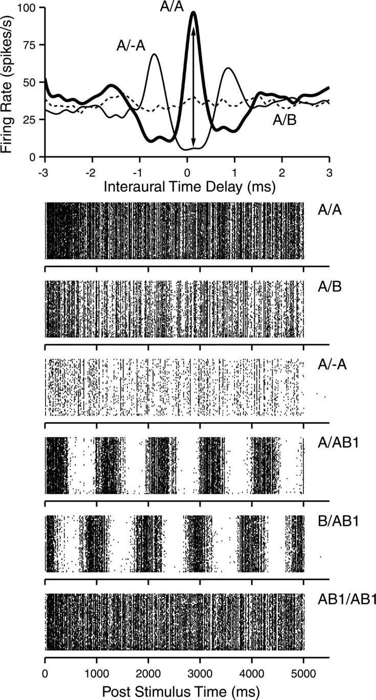
Responses of one neuron to static and dynamic stimuli. Top, Noise-delay functions for correlated noise (A/A), uncorrelated noise (A/B), and anticorrelated noise (A/–A). The double arrow at the best delay (150 μs) indicates the expected modulation in firing rate to dynamic stimuli. Stimulus parameters (duration/repetition interval × number of repetitions): 1/1.5 s × 3. Middle, Bottom, Dot rasters of responses to the stimuli indicated next to each panel. Stimulus parameters: 5/6 s × 50. ITD was 150 μs, and effective SPL was 45 dB in all cases, which was ∼ 40 dB above rate threshold. CF was 800 Hz. Additional data for this neuron are shown in Figure 8A–C.

The expectation for the response to stimuli with varying interaural correlation is illustrated by the vertical line and arrowheads at the ITD of 150 μs. We expect a response varying between the high firing rate when the waveforms at the two ears are correlated and the low firing rate when they are anticorrelated. The dot rasters in Figure 2 illustrate that this is indeed the case. The top three raster panels show responses to correlated, uncorrelated, and anticorrelated noise, presented at the best delay (150 μs). When the AB1 stimulus at the ipsilateral ear is paired with the A or B stimulus at the contralateral ear, again with an ITD of 150 μs, firing rate clearly varies with a 1 Hz periodicity and thus with the degree of interaural correlation. The A/AB1 stimulus pair starts out uncorrelated, reaches peak correlation at 0.25 cycles, and peak anticorrelation at 0.75 cycles (compare with Fig. 1, rightmost panel). Likewise, the response starts at an intermediate level, increases to a maximum in the first 500 ms, and drops to a minimum in the subsequent 500 ms: it tracks the time-varying correlation between the binaural stimuli. In the B/AB1 stimulus, peak correlation is at phase 0 and 1 cycle and peak anticorrelation at 0.5 cycle: again the response rate follows the same pattern. Finally, the response to an AB1/AB1 pair is sustained, indicating that the rate modulation at 1 Hz is a true binaural effect. The vector averages of the data for the A/AB1 and B/AB1 stimuli also show a one-quarter cycle phase difference: R and ϕ values were 0.67 and 0.22 cycle for A/AB1 and 0.64 and 0.98 cycle for B/AB1. For all the other stimulus pairs shown in this figure, R values are <0.01 and not significant.

In seven cells, we studied the responses to dynamic stimuli presented at ITDs that differ from the best delay. Noise-delay functions to static stimuli are usually modeled by a cross-correlation of bandpassed and half-wave-rectified binaural signals that undergo a neural delay that may differ for left and right side. This difference or “internal delay” is negated at the best delay, at which the effective stimuli, i.e., the signals received by the binaural coincidence detector, are maximally correlated. For ITDs that differ from the best delay, the effective stimuli are to varying extents decorrelated by peripheral processing. If the stimuli with varying interaural correlation are presented at ITDs near nodal points in the noise-delay functions, i.e., ITDs at which the response rate to correlated and anticorrelated noise is identical, we expect a corresponding decrease in synchronization at the modulation frequency. At ITDs in which the response magnitude to correlated stimuli is lower than that to anticorrelated stimuli, we expect a modulated response but with a 0.5 cycle change in response phase. The results are as expected and are illustrated for three cells in Figure 3, which shows responses to static (bottom row) and dynamic (top two rows) noise stimuli. R and ϕ values to the modulation frequency were obtained from responses over a range of ITDs. High R values are indeed obtained at ITDs with large firing rate differences for correlated and anticorrelated static stimuli and small or insignificant values (filled circles) at ITDs near nodal points. The phase of the response is near 0.25 cycle if the static A/A response is high and near 0.75 cycle if the static A/–A response is high. These data therefore confirm our expectation that the largest response modulation is obtained at ITDs to which there is also the largest difference in response rate to static stimuli. The data shown in the remainder of this paper were all obtained at the best delay, except when stated otherwise.

Figure 3.

ITD dependence of synchronization to dynamic stimuli in three cells. For each cell (column), the bottom row shows the responses at different ITDs to statics timuli, the middle row the synchronization magnitude to dynamic stimuli, and the top row the synchronization phase. Phase values are not shown for data with insignificant synchronization, indicated with filled symbols in the middle row. Effective SPLs were 74 dB (A), 48 dB (B), and 60 dB (C); f_r was 5 Hz (A), 1 Hz (B), and 10 Hz (C). CFs were all 950 Hz.

For each cell, we also determined the SPL at which maximal response modulation was present, by running a level series of the dynamic stimulus, usually in 5 dB steps with f_r at 1 Hz. For the vast majority of cells, the results were unremarkable: R tended to be maximal at low levels but generally changed little with SPL; ϕ was virtually constant near 0.25 cycle. Figure 4 illustrates some of the variety seen in the rate and in the strength and phase of synchrony to f_r. In some cases, especially at CFs > 1 kHz, R showed a stronger dependence on SPL, which was usually associated with peak doubling, discussed below.

Figure 4.

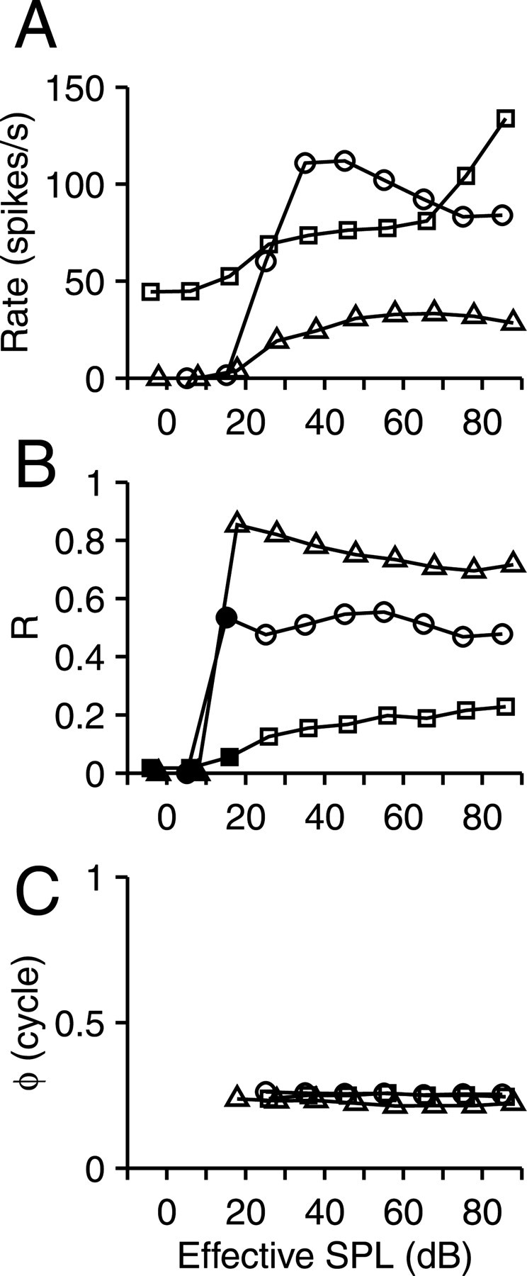
SPL dependence of synchronization to dynamic stimuli. Representative examples in three neurons of change in average firing rate (A) and magnitude (B) and phase (C) of synchronization to f_r, which here was at 1 Hz. Phase values are not shown for data with insignificant synchronization, indicated with filled symbols in B. CF and best delay were (circles, squares, and triangles) 695, 1900, and 950 Hz and 0, 100, and 0 μs.

IC neurons: transfer functions

Figure 5 shows a representative example of responses to the OSCOR stimulus over a range of modulation frequencies (CF was 950 Hz; best delay was 300 μs). Synchronization to the A/ABf_r stimuli is illustrated with period histograms in the left column of A and is clearly present at 5 and 20 Hz, then declines from 100 to 400 Hz, and is insignificant at 500 Hz. The histograms also show a progressive phase lag. To rule out the possibility of artifactual phase locking, not based on degree of interaural correlation but on some other, spurious component in the AB stimulus (e.g., amplitude modulation), responses to a control ABf_r/ABf_r stimulus were obtained. As expected, the response to this correlated stimulus remains high throughout the modulation period (Fig. 5A, right column): there is no evidence of temporal structure synchronized to the modulator frequency.

Figure 5.

Responses of one neuron to stimulus of varying interaural correlation at increasing frequency. A, Period histograms to modulated A/AB f_r stimuli (left column) and AB f_r/ABf_r control stimuli (right column), at the f_r indicated above each pair of histograms. Axis scales on bottom left apply to all histograms. The average rate (B), synchronization magnitude (C), and phase (D) are shown for all responses to the A/ABf_r (circles) and ABf_r/ABf_r (triangles) stimuli. Abscissa in D applies to B–D, but B and C are logarithmic. The filled symbols in C indicate insignificant phase locking. CF was 950 Hz, best delay was 100μs, and effective SPL was 44 dB, which was ∼40 dB above the rate threshold.

R values to the A/ABf_r stimuli as a function of modulation frequency, henceforth referred to as f_r transfer functions, are shown in C (circles). Values that are not statistically significant are shown with filled symbols. None of the values obtained to the ABf_r/ABf_r control stimulus were significant (filled triangles), and this was the case for the 14 neurons in which this control was tested. We extracted several metrics from the f_r transfer functions. The best modulation frequency is the f_r yielding the maximal R value, R_max. We also determined the 6 dB upper cutoff frequency (dotted lines at intersection of horizontal line at R_max/2 with linear interpolation between neighboring data points) and the highest f_r at which significant modulation was obtained.

B and D show average firing rate (circles, triangles) and synchronization phase ϕ (only for responses with significant modulation). As mentioned in Materials and Methods, phase values show an increasing lag with increasing f_r, and, from the phase plot, we determined a pure time delay that captures the total delay between modulation in the stimulus and the response, which is 8.52 ms in the example of Figure 5D. Firing rate showed little change with f_r.

We obtained a total of 246 f_r transfer functions in 95 IC neurons, often at different SPLs. Transfer functions to f_r for all cells (one per neuron) are shown in the top four panels of Figure 6, grouped according to CF and including only the statistically significant points. A shallow high-pass slope is often present, but the basic shape is low-pass in most cases. It is immediately clear that the range of significant f_r values extends much higher than the psychophysical detection range, at which sensitivity is lost above 50 Hz (Grantham, 1982). Several neurons show synchronization at 500 and at 750 Hz and one neuron even at 1 kHz. At the higher CFs (Fig. 6B,E), the transfer functions extend to high f_r values, but synchronization values are often very low throughout the range of significant phase locking. The bottom panels show the average rate (Fig. 6C) and phase (Fig. 6F) for all neurons: the population behavior is generally as was shown for the neuron of Figure 5. Average rate is often low because the stimulus was often at low suprathreshold levels, when these gave the highest synchronization values, as discussed with Figure 4. After subtraction of the best-fitting pure time delay (see Materials and Methods; these delays are discussed below in Fig. 11), the phase curves are near horizontal, with a y-intercept near 0.25 for the A/ABf_r stimulus (compare with Fig. 1) or 0.75 in two cases in which the stimulus was placed at the “worst” ITD.

Figure 6.

Population f_r transfer functions to stimulus with varying interaural correlation. A, B, D, E, Synchronization magnitude R, grouped in the CF ranges shown above each panel. Ordinate of A and B also applies to D and E. Only statistically significant values are shown. The dashed line in E is from the neuron with the highest CF in our sample. C, F, Average rate and synchronization phase ϕ for all neurons shown in top four panels. The phase curves show residual values after subtraction of a pure time delay, which best captured the slope in the phase-frequency function. To improve traceability of individual curves, three-point triangular smoothing was applied to the synchronization curves in the top panels, and cubic splines are shown with omission of markers for individual data points. One dataset with average rate ∼130 spikes/s was omitted in C.

Figure 11.

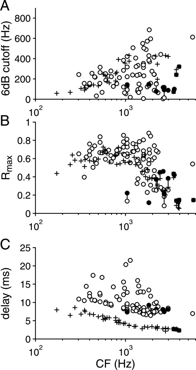
Population data for AN fibers (plus signs, filled squares) and IC neurons (circles, filled circles). Each panel shows the population distribution of one metric obtained from the f_r transfer functions. In seven IC neurons and six AN fibers, R_max values were higher at 2f_r (filled circles, filled squares) than at f_r (empty circles, plus signs): both values are shown joined with a vertical line.

That some of the transfer functions in Figure 6 show low synchronization values, sometimes over the entire f_r range, deserves additional comment. Period histograms of such responses binned at f_r reveal double peaks, as illustrated for one cell in Figure 7A (left column). Period histograms from the same responses binned at 2f_r are also shown (right column). Clearly, synchronization to the varying interaural correlation is present but at twice the modulation frequency. Significant synchronization extends to 100 Hz (Fig. 7C), and, over the range of 1–10 Hz, the second harmonic (squares) in the response exceeds the component at f_r (circles).

Figure 7.

Double-peaked period histograms for responses to varying interaural correlation. A, Left column, Period histograms at the oscillation frequencies indicated, binned at f_r. Right column, Period histograms for same responses but binned at 2f_r. Noise-delay functions (B) and synchronization functions (C) are graphed following the same conventions as in Figures 2 and 5, respectively, but an additional synchronization function binnedat 2 f_r is shown (squares). CF was 2.5 kHz, and effective SPL was 62 dB (20 dB above rate threshold). Responses in A and C were obtained at ITD of 0 μs.

An explanation for the double-peak behavior is found in the noise-delay functions (Fig. 7B); the responses to correlated (A/A) and anticorrelated (A/–A) noise show a “central mound” of increased firing rate over the same ITD range, which is absent in the response to uncorrelated noise (A/B). The dynamic responses in A were obtained at an ITD of 0 μs. At that ITD, the static response is highest to the correlated noise (A/A), lowest to the uncorrelated noise (A/B), and of intermediate value to the anticorrelated noise (A/–A). Likewise, to the stimulus with varying correlation (A/AB) (Fig. 8A), the response is high during phase values with high correlation (at ∼0.25 cycle; compare with Fig. 1), low for phase values with zero correlation (at 0 and 0.5 cycle), and high again for phase values with anticorrelation (at ∼0.75 cycle, the actual phase values are somewhat offset because of conduction delays).

Figure 8.

Tuning to f_r. A–C, Tuning of one cell in synchronization but not in average rate, at different SPLs. The rate threshold was at an effective SPL of 6 dB. Effective SPLs (○, ▵, □, and ▿) were 26, 46, 66, and 86 dB. Delays measured from the phase functions were 12.2, 11.6, 11.5, and 12 ms. CF was 800 Hz; best delay was 150 μs. D–F, Tuning in average rate but not in synchronization, in three neurons. CF, effective SPL, delay, and best delay were as follows (○, □, and ▵): 1820, 1045, and 1900 Hz; 49, 40, and 62 dB; 13.4, 9.1, and 11.7 ms; and 100, 200, and 100 μs. Ordinates of the left column also apply to the right column.

The occurrence of peak doubling was not an all-or-none phenomenon for a given neuron: it was often more pronounced at certain SPLs and f_r values than at others, but it was clearly associated with the “polarity tolerance” in noise-delay functions described previously (Joris, 2003). It thus reflects instances in which the ITD sensitivity is dominated by envelope components rather than by fine structure. Some degree of peak doubling was observed in 19 cells, which all had CFs ≥1 kHz. We also analyzed all OSCOR data at the doubled binning frequency (2f_r), but, in most cases with peak doubling, the synchronization values at 2f_r were smaller than those at f_r. In the additional analyses, phase locking at f_r is reported, except when indicated otherwise.

It is interesting to observe that a minority of neurons showed some degree of bandpass tuning to f_r in terms of either synchronization or average rate. Figure 8 (left) shows different f_r transfer functions of one neuron. With increasing SPL, R values at low f_r tend to decrease so that the transfer function becomes more bandpass in shape (Fig. 8B). In contrast, average rate is little affected by f_r at all SPLs (Fig. 8A), and phase is unchanged (Fig. 8C). Other neurons for which transfer functions were obtained at different SPL showed a similar tendency toward bandpass tuning at high SPL, although not as clearly as in the neuron illustrated. Some neurons showed tuning in average rate (Fig. 8D), whereas their f_r transfer functions were low-pass (Fig. 8E). Because the stimuli in all of these cases are monaurally “featureless,” the bandpass tuning in rate must reflect binaural interaction and must thus arise at or above the level of the MSO.

Comparison with auditory nerve

To enable comparison of the IC data with the AN, we obtained responses of AN fibers to OSCOR stimuli and performed a coincidence analysis. The procedure is illustrated in Figure 9. PST histograms are shown in the left column for one fiber to 10 repetitions of the unmodulated stimuli (A, –A, B, and –B) and a mixed stimulus (AB1). As expected, none of these responses show any modulation at 1 Hz. When only the spikes that are coincident (in bins of 50 μs) between the spike trains to the modulated and the four unmodulated stimuli are retrieved (Fig. 9B), the resulting PST histograms are clearly modulated and show the expected difference in phase for the various combinations (compare with Fig. 2). Note that the ordinate shows the rate of coincident spikes, which is much lower than the actual response rate to the individual stimuli (left column). From the coincidence spike trains to these four pairs, we constructed period histograms and a pooled period histogram (Fig. 9C). The pooling consisted of phase shifting the period histograms to conform to the A/ABf_r stimulus. Thus, the period histograms of the coincident spike trains to the –A/ABf_r stimulus were shifted by 0.5 cycle, those of the B/ABf_r stimuli by –0.25 cycle, and those of the –B/ABf_r stimuli by 0.25 cycle. The rationale for the use of four referent stimuli and the pooling of histograms is the low rate of coincidences caused by our narrow 50 μs coincidence window. We used such a conservative (i.e., short) window to count coincidences to avoid reduction of the upper frequency limit of phase locking to the OSCOR stimuli by temporal integration in the analysis window. Pooling increases the total number of coincidences but is not essential to any of the conclusions drawn. The procedure illustrated in Figure 9 results in a single R and ϕ value at 1 Hz. The additional analysis of these values, for the range of oscillation frequencies studied, was identical to that of the IC data.

Figure 9.

Coincidence analysis to study phase locking to OSCOR stimuli in the auditory nerve. A, PST histograms to 10 repetitions of the stimulus indicated next to each panel. B, PST histograms of coincident spikes, based on 100 permutations of responses to the pairs of stimuli indicated next to each panel. The procedure for constructing the histograms in A and B is schematically illustrated above each column. For the PST histograms, all spike times are counted. For the histograms of coincident spikes, only pairs of identical or coincident spike times (within a 50μs bin) are counted. C, Period histograms for the top four PST histograms of B, with indication of synchronization magnitude and phase (cycle). The bottom period histogram is a pooled average of the top four histograms, after phase shifting (see Results). Responses were obtained at an effective SPL of 45 dB. CF was 274 Hz. Number of bins is 60 (left column), 50 (middle), and 64 (right). Axis scales of the bottom row apply to all other rows.

Synchronization of AN fibers to the OSCOR stimuli shows similar features as in the IC. Figure 10 illustrates f_r transfer functions, grouped according to CF as in Figure 6. Here, too, phase locking to f_r extends to higher frequencies in high-CF than in low-CF fibers, and fibers with CF >1 kHz often show poor phase locking (Fig. 10B,E). Although not further illustrated here, these fibers showed the same phenomenon of peak doubling as IC neurons (in 28 fibers). Rate and phase, compensated for a pure time delay, showed even less dependence on f_r than in the IC (Fig. 10C,F). Perhaps the most striking difference in the shape of the transfer functions, between AN and IC, is the total lack of high-pass slopes in the AN, whereas some degree of such slope (albeit shallow) is common in the IC (Fig. 6). Such slopes are therefore not attributable to the timing information in the AN and probably reflect a dynamic process at the site of binaural interaction or higher up.

Figure 10.

AN f_r transfer functions, in the same format as in Figure 6. A, B, D, E, Synchronization magnitude R, grouped according to CF as indicated. C, F, Average coincidence rate and synchronization ϕ for all neurons. Four neurons for which coincidence rate was >10/s are omitted in C. The phase curves show residual values after subtraction of a pure time delay.

Figure 11 presents an overview of the different metrics calculated from the f_r transfer functions, plotted as a function of CF, for both IC and AN neurons: 6 dB upper cutoff frequencies (Fig. 11A), R_max (Fig. 11B), and delay (Fig. 11C). As expected, the upper frequency cutoffs increase with CF, up to ∼2 kHz. The increase was similar for the AN and the IC and was also present when the highest significant f_r was graphed versus CF (data not shown). The highest cutoffs, at CFs between 1 and 2 kHz, were all obtained in the IC, but note that there is a shortage of AN measurements in that CF region. The distributions in AN and IC differ in that the increase in cutoff frequency is rather uniform in the AN, whereas in the IC, low cutoffs are present at all CFs. At CFs >1 kHz, many of these neurons also show peak doubling, and filled symbols in Figure 11 indicate a subset of such neurons: neurons for which R_max to 2f_r was larger than R_max to f_r. For these neurons, values obtained by binning at f_r (circles and plus signs) and at 2f_r (filled circles and filled squares) are both shown, if statistically significant, and joined with a vertical line. Note that all cutoffs are specified in terms of stimulus frequency (f_r) and not in terms of binning frequency (2f_r): responses with peak doubling actually oscillate at twice the cutoff frequency shown.

High R_max values (Fig. 11B) are found in the IC up to CFs of 2 kHz, but, starting at 1 kHz, low values occur as well. The distribution in the AN is tighter than in the IC and, as expected, is rather similar in overall shape to the distribution of R_max values for phase locking to pure tones near CF (Johnson, 1980). Over much of the CF range, R_max values reach higher values in the IC than in the AN.

In the AN, the delays measured from the ϕ versus f_r responses behaved orderly with CF and are consistent with other AN delay measurements based on sustained responses (Joris and Yin, 1992). The distribution in the IC is more scattered, but the majority of fibers follow a distribution similar to the AN, displaced vertically by ∼4 ms.

We encountered one IC neuron with high CF (above the phase-locking range, 5570 Hz) that showed envelope-dominated ITD sensitivity at low SPLs and poor response modulation to the OSCOR stimuli. However, at the highest SPL tested (effective SPL of 90 dB, ∼60 dB relative to rate threshold), the response was dominated by fine structure and showed response modulation at f_r over a wide range (Fig. 6D, dashed line). Similar dominance of the response to broadband noise by fine structure has also been observed in monaural high-CF neurons (Louage et al., 2005), also at high SPLs.

Comparison with binaural beat responses

A binaural stimulus with dynamic properties that has received much attention is the BB (Kuwada et al., 1979; Yin and Kuwada, 1983; Spitzer and Semple, 1991, 1993; Batra et al., 1997). This stimulus produces a periodic change in interaural phase difference (IPD), and the rate of change increases with the beat frequency f_b. We obtained BB responses over a range of f_b in eight IC neurons to compare with the OSCOR responses. One tone was fixed at CF, and another tone was placed above CF at increasing frequency or below CF at decreasing frequency, so that f_b increased in linear steps. Figure 12 shows a representative response for one neuron. As in most neurons, average rate (Fig. 12A) and phase (Fig. 12C) of synchronization (after subtraction of a delay) in this cell changed little for the OSCOR stimulus (triangles). In contrast, average rate to the BB (circles) showed an overall decrease with increasing f_b, usually in a nonmonotonic form as for the example illustrated (Fig. 12A). The phase curves were less linear for the BB than for the OSCOR responses (Fig. 12C) and showed marked curvature in a few cells. The most interesting comparison, however, is in the synchronization curve (Fig. 12B). The synchronization to f_b was stronger than to f_r, but the two curves converge so that the upper limit of synchronization to f_b is similar to that to f_r, at 591 and 500 Hz, respectively. For the eight neurons studied, the highest significant frequencies to OSCOR and BB stimuli were well correlated (r = 0.82), and the same was true for delay (r = 0.96). For both metrics, linear regressions had slopes near 1 (0.94 and 0.92). This small sample thus suggests that modulation of IPD and correlation are limited by common processes. Note that the upper f_b limit in Figure 12B is higher than the upper limit reported previously [80 Hz (Yin and Kuwada, 1983)]. This was the case in seven of eight neurons studied, with the highest significant f_b at 1 kHz.

Figure 12.

Comparison of responses to OSCOR stimuli and to BBs: response rate (A), synchronization magnitude (B), and phase (C) of one IC neuron to OSCOR (triangles) and BB (circles) stimuli. The abscissa indicates the frequency of oscillation in correlation (for OSCOR) or of the beat (for BB). Phase is after subtraction of 8.4 ms for BB and 8.2 ms for OSCOR. CF was 1820 Hz. SPL was 70 dB for the BB stimuli (44 dB above rate threshold) and at an effective SPL of 46 dB for the OSCOR stimuli. In B and C, only statistically significant values are shown.

Discussion

Our main observation is that, at the level of the midbrain examined, most neurons can temporally “follow” oscillations in interaural correlation at frequencies that far exceed human psychophysical abilities. In fact, a large percentage of neurons showed maximal synchronization at modulation frequencies (f_r of 20–50 Hz) at which human detection ceases to exist (Grantham, 1982). There was large overlap with cutoffs and maximal synchronization values obtained with a coincidence analysis of AN fibers.

The temporal responses of IC neurons as a function of f_r were rather stereotyped. The magnitude of the f_r transfer function had a low-pass shape in most neurons (Fig. 6). The population showed high maximal synchronization values (Fig. 12B) and a steady increase in upper cutoff frequencies (Fig. 11A) with CF up to CFs of ∼2 kHz. Starting at CFs of ∼1 kHz, maximal synchronization and cutoff values were often low and showed peak doubling (Figs. 7, 11). This was always associated with polarity tolerance in the noise-delay function (Joris, 2003) and therefore indicated envelope ITD sensitivity. Note that part of the decrease in R_max at mid-CFs (even after adjusting the binning frequency to 2f_r) is attributable to the change in temporal waveform of the interaural correlation as it changes from being carried by fine structure to envelope. Broadly similar trends were seen in the transfer functions calculated from coincidence patterns of the AN fibers, obtained from the same stimuli.

The monaural hare and the binaural slug

In the psychophysical literature, it is customary to paint a contrasting picture of the binaural slug and the monaural hare. It should be emphasized that both extremes are surprising from a physiological point of view: not only the sluggishness of the binaural system but also the very high modulation frequencies (2.5 kHz) at which modulation can be detected monaurally in wideband signals (Viemeister and Plack, 1993; Eddins and Green, 1995). This is near the edge of temporal modulation coding at high CFs in the cat auditory nerve (Joris et al., 2004), and a higher limit in the human auditory nerve than in the cat is unlikely (Shera et al., 2002). Moreover, the psychophysical cutoff frequency for AM detection does not depend on stimulus center frequency (Strickland and Viemeister, 1997; Eddins, 1999), and psychophysical models suggest that detection thresholds can only be accounted for if information is extracted over wide frequency regions: wider than compatible with estimated cochlear filter widths. These observations question whether phase locking at the modulation frequency, as measured with traditional physiological paradigms, is the primary cue on which behavioral AM detection is based.

Whereas AM detection is present at higher modulation frequencies than expected based on envelope phase locking, behavioral detection of dynamic changes in correlation certainly vanishes at much lower modulation frequencies than expected from physiological temporal properties, as clearly shown by our AN and IC data. A simple neural substrate of binaural sluggishness would be that neurons show a high R_max value at low f_r combined with a very low cutoff frequency, but such neurons were rare (Figs. 6, 11A,B). Of course it is quite likely, as is the case for AM coding (for review, see Joris et al., 2004), that there is a systematic loss of synchronization to high modulation frequencies along the auditory neuraxis. Such progressive low-pass filtering could constitute a basis for sluggishness. Note, however, that the relationship between monaural and binaural phase locking appears to be reversed at higher levels in the auditory pathway: cortical neurons are more sluggish monaurally (synchronization to AM) than binaurally (synchronization to the BB) (Reale and Brugge, 1990), whereas psychophysically, modulation detection is sluggish binaurally but fast monaurally. Although these comparisons suggest an interesting double dissociation between psychophysical and physiological findings, they are necessarily sketchy because of lack of data at many levels, particularly for animal behavior. Monaural modulation detection in laboratory animals is of the same order of magnitude as in humans (Moody, 1994), but to our knowledge there are no comparative data on binaural sluggishness.

In summary, although at this time the data on binaural modulation processing are limited, they hint at qualitative differences in the processing of binaural and monaural modulation at the level of the midbrain and above.

A hypothesis: inaccessible temporal coding at the level of the IC

Our physiological findings do not pinpoint the source of sluggishness but show that, at the level of the IC, there is temporal encoding of fluctuations an order of magnitude faster than can be detected behaviorally. This encoding does not seem to be “read out” appropriately for perception. We hypothesize that, already at the level of the IC, these fluctuations are in a form that is not further decoded by the CNS, except at the lowest modulation frequencies (10–20 Hz or lower), at which multiple spikes can be fired per modulation cycle and at which these fluctuations are thus coded as short-term changes in average firing rate. In essence, we propose that, after their unavoidable generation at the level of binaural interaction (the MSO), there is no neural substrate to recode these temporal fluctuations in a different form (e.g., a rate code) and that this constitutes a low-pass sluggishness filter.

Before giving our reasoning, we draw attention to the modulations in firing rate that are always present in responses to noise. For example, the response to the correlated A/A noise pair in Figure 2 (top dot raster) shows prominent vertically (thus temporally) aligned spike occurrences, which at least partly reflect pseudorandom amplitude modulations at a monaural level consequent to cochlear bandpass filtering (Joris, 2003). Such modulations are also present in response to the uncorrelated A/B noise pair (Fig. 2, second dot raster). Here, additional sources of modulations in spike rate are pseudorandom, stimulus-based binaural fluctuations in interaural correlation. With the OSCOR stimulus, sinusoidal fluctuations in interaural correlation provide yet a third source of temporal structure in these responses. At low f_r (Fig. 2, A/AB1 and B/AB1), these sinusoidal fluctuations result in visibly changing spike densities. At high f_r, however, these sinusoidal fluctuations are only revealed by an averaging process in which the pseudorandom fluctuations smooth out. In our analysis, this occurs through the temporal averaging inherent in cycle histograms (Fig. 5A) or in Fourier analysis. Note that here an average of n response cycles of one fiber does not result in the same histogram as an average of one response cycle of n fibers (of the same CF). In the latter case, the random fluctuations will not smooth out, to the extent that they are stimulus based and thus correlated in fibers of the same CF. To disambiguate random fluctuations in spike rate from fluctuations attributable to short-term changes in correlation, the only option is to average across CFs. This seems to be the strategy taken by the monaural system in modulation detection (Viemeister and Plack, 1993; Eddins and Green, 1995).

An important difference between monaural AM processing and binaural correlation processing is that monaural fluctuations are “right there” in all their richness in the AN input to the first synaptic stage of the CNS. Although it is unsettled which cell types and circuits are necessary and sufficient for monaural temporal analysis, clearly there is a rich assortment of response patterns between the AN and the IC. Cochlear nucleus (CN) neurons are differently endowed with intrinsic properties and circuit connections (Oertel, 1997); the extent to which they differentially respond to the fine-grained temporal information available within and across AN fibers has only been partially explored (Heinz et al., 2001). This fine-grained information is no longer available at the level of the IC. Binaural correlation requires several processing steps before being encoded in the form of a change in instantaneous spike rate at the level of the MSO. Neural machinery that is available at the CN to extract information from temporal patterns may have no equivalent at the level of the output targets of the MSO. At the same time, the presence of internal delays effectively introduces an additional dimension (besides CF) in which binaural neurons differ, especially at very low CFs (McAlpine et al., 2001; Hancock and Delgutte, 2004; Joris et al., 2005b). This extra dimension makes the temporal pattern of phase locking to f_r across the population complex because neurons can be in phase or in antiphase depending not only on CF and latency (Fig. 11C) but also on ITD (Fig. 3).

The computational complexity to extract fast binaural modulations, especially if integration across CFs is required as argued above, contrasts with the expected benefits. Indeed, it may be argued that there is a functional reason to reduce rather than enhance binaural temporal resolution. It is easy to see that AM is such a fundamental property of auditory signals that its detection is useful for a variety of tasks, but this is much less clear for detection of dynamic changes in correlation. With a single source in an anechoic environment, changes in interaural correlation are small in speed and depth; rapid changes in binaural parameters require multiple sources or echoic environments. Recent modeling studies suggest that, under these circumstances, it may be beneficial to temporally integrate the output of ITD-sensitive neurons (Shinn-Cunningham and Kawakyu, 2003).

References

- Batra R, Kuwada S, Stanford TR (1989) Temporal coding of envelopes and their interaural delays in the inferior colliculus of the unanesthetized rabbit. J Neurophysiol 61: 257–268. [DOI] [PubMed] [Google Scholar]
- Batra R, Kuwada S, Fitzpatrick DC (1997) Sensitivity to interaural temporal disparities of low- and high-frequency neurons in the superior olivary complex. I. Heterogeneity of responses. J Neurophysiol 78: 1222–1236. [DOI] [PubMed] [Google Scholar]
- Bernstein LR, Trahiotis C, Akeroyd MA, Hartung K (2001) Sensitivity to brief changes of interaural time and interaural intensity. J Acoust Soc Am 109: 1604–1615. [DOI] [PubMed] [Google Scholar]
- Boehnke SE, Hall SE, Marquardt T (2002) Detection of static and dynamic changes in interaural correlation. J Acoust Soc Am 112: 1617–1626. [DOI] [PubMed] [Google Scholar]
- Chan JK, Musicant AD, Hind JE (1993) An insert earphone system for delivery of spectrally shaped signals for physiological studies. J Acoust Soc Am 93: 1496–1501. [DOI] [PubMed] [Google Scholar]
- Culling JF, Colburn HS (2000) Binaural sluggishness in the perception of tone sequences and speech in noise. J Acoust Soc Am 107: 517–527. [DOI] [PubMed] [Google Scholar]
- Culling JF, Summerfield Q (1998) Measurements of the binaural temporal window using a detection task. J Acoust Soc Am 103: 3540–3553. [Google Scholar]
- Eddins DA (1999) Amplitude-modulation detection at low- and high-audio frequencies. J Acoust Soc Am 105: 829–837. [DOI] [PubMed] [Google Scholar]
- Eddins DA, Green DM (1995) Temporal integration and temporal resolution. In: Hearing (Moore BCJ, ed), pp 207–242. San Diego: Academic.
- Gibson DJ (1982) Interaural crosstalk in the cat. Hear Res 7: 325–333. [DOI] [PubMed] [Google Scholar]
- Goldberg JM, Brown PB (1969) Response of binaural neurons of dog superior olivary complex to dichotic tonal stimuli: some physiological mechanisms of sound localization. J Neurophysiol 22: 613–636. [DOI] [PubMed] [Google Scholar]
- Grantham DW (1982) Detectability of time-varying interaural correlation in narrow-band noise stimuli. J Acoust Soc Am 72: 1178–1184. [DOI] [PubMed] [Google Scholar]
- Grantham DW, Wightman FL (1978) Detectability of varying interaural temporal differences. J Acoust Soc Am 63: 511–523. [DOI] [PubMed] [Google Scholar]
- Grantham DW, Wightman FL (1979) Detectability of a pulsed tone in the presence of a masker with time-varying interaural correlation. J Acoust Soc Am 65: 1509–1517. [DOI] [PubMed] [Google Scholar]
- Hancock KE, Delgutte B (2004) A physiologically based model of interaural time difference discrimination. J Neurosci 24: 7110–7117. [DOI] [PMC free article] [PubMed] [Google Scholar]
- Heinz MG, Colburn HS, Carney LHC (2001) Rate and timing cues associated with the cochlear amplifier: level discrimination based on monaural cross-frequency coincidence detection. J Acoust Soc Am 110: 2065–2084. [DOI] [PubMed] [Google Scholar]
- Johnson DH (1980) The relationship between spike rate and synchrony in responses of auditory-nerve fibers to single tones. J Acoust Soc Am 68: 1115–1122. [DOI] [PubMed] [Google Scholar]
- Joris PX (1996) Brainstem responses to modulated interaural cues. Acta Acustica united with Acustica 82: S97. [Google Scholar]
- Joris PX (2003) Interaural time sensitivity dominated by cochlea-induced envelope patterns. J Neurosci 23: 6345–6350. [DOI] [PMC free article] [PubMed] [Google Scholar]
- Joris PX, Smith PH (1998) Temporal and binaural properties in dorsal cochlear nucleus and its output tract. J Neurosci 18: 10157–10170. [DOI] [PMC free article] [PubMed] [Google Scholar]
- Joris PX, Yin TCT (1992) Responses to amplitude-modulated tones in the auditory nerve of the cat. J Acoust Soc Am 91: 215–232. [DOI] [PubMed] [Google Scholar]
- Joris PX, Schreiner CE, Rees A (2004) Neural processing of amplitude-modulated sounds. Physiol Rev 84: 541–577. [DOI] [PubMed] [Google Scholar]
- Joris PX, Van de Sande B, van der Heijden M (2005a) Temporal damping in response to broadband noise. I. Inferior colliculus. J Neurophysiol 93: 1857–1870. [DOI] [PubMed] [Google Scholar]
- Joris PX, van der Heijden M, Louage DH, Van de Sande B, van Kerckhoven S (2005b) Dependence of binaural and cochlear “best delays” on characteristic frequency. In: Auditory signal processing: physiology, psychoacoustics, and models (Pressnitzer D, de Cheveigné A, McAdams S, Collet L, eds), pp 478–484. New York: Springer.
- Kollmeier B, Gilkey RH (1990) Binaural forward and backward masking: evidence for sluggishness in binaural detection. J Acoust Soc Am 87: 1709–1719. [DOI] [PubMed] [Google Scholar]
- Krishna SB, Semple MN (2000) Auditory temporal processing: responses to sinusoidally amplitude-modulated tones in the inferior colliculus. J Neurophysiol 84: 255–273. [DOI] [PubMed] [Google Scholar]
- Kuwada S, Yin TCT, Wickesberg RE (1979) Response of cat inferior colliculus neurons to binaural beat stimuli: possible mechanisms for sound localization. Science 206: 586–588. [DOI] [PubMed] [Google Scholar]
- Kuwada S, Yin TCT, Syka J, Buunen TJF, Wickesberg RE (1984) Binaural interaction in low-frequency neurons in inferior colliculus of the cat. IV. Comparison of monaural and binaural response properties. J Neurophysiol 51: 1306–1325. [DOI] [PubMed] [Google Scholar]
- Louage DH, van der Heijden M, Joris PX (2004) Temporal properties of responses to broadband noise in the auditory nerve. J Neurophysiol 91: 2051–2065. [DOI] [PubMed] [Google Scholar]
- Louage DH, van der Heijden M, Joris PX (2005) Enhanced temporal response properties of anteroventral cochlear nucleus neurons to broadband noise. J Neurosci 25: 1560–1570. [DOI] [PMC free article] [PubMed] [Google Scholar]
- Mardia KV, Jupp PE (1999) Directional statistics. New York: Wiley.
- McAlpine D, Jiang D, Palmer A (2001) A neural code for low-frequency sound localization in mammals. Nat Neurosci 4: 396–401. [DOI] [PubMed] [Google Scholar]
- Moody D (1994) Detection and discrimination of amplitude-modulated signals by macaque monkeys. J Acoust Soc Am 95: 3499–3510. [DOI] [PubMed] [Google Scholar]
- Nienborg H, Bridge H, Parker AJ, Cumming BG (2005) Neuronal computation of disparity in V1 limits temporal resolution for detecting disparity modulation. J Neurosci 25: 10207–10219. [DOI] [PMC free article] [PubMed] [Google Scholar]
- Oertel D (1997) Encoding of timing in the brain stem auditory nuclei of vertebrates. Neuron 19: 959–962. [DOI] [PubMed] [Google Scholar]
- Oliver DL (2005) Neuronal organization in the inferior colliculus. In: The inferior colliculus (Winer JA, Schreiner CE, eds), pp 69–114. New York: Springer.
- Olson RE, Yee D, Rhode WS (1985) Digital system, Version II. In: Madison: Medical Electronics Laboratory and Department of Neurophysiology, University of Wisconsin–Madison.
- Reale RA, Brugge JF (1990) Auditory cortical neurons are sensitive to static and continuously changing interaural phase cues. J Neurophysiol 64: 1247–1260. [DOI] [PubMed] [Google Scholar]
- Rodenburg M (1977) Investigation of temporal effects with amplitude modulated signals. In: Psychophysics and physiology of hearing (Evans EF, Wilson JP, eds), pp 429–437. London: Academic.
- Shera CA, Guinan JJ, Oxenham AJ (2002) Revised estimates of human cochlear tuning from otoacoustic and behavioral measurements. Proc Natl Acad Sci USA 99: 3318–3323. [DOI] [PMC free article] [PubMed] [Google Scholar]
- Shinn-Cunningham B, Kawakyu K (2003) Neural representation of source direction in reverberant space. In: IEEE workshop on applications of signal processing to audio and acoustics, pp 79–82. New Paltz, NY: IEEE.
- Spitzer MW, Semple MN (1991) Interaural phase coding in auditory midbrain: influence of dynamic stimulus features. Science 254: 721–724. [DOI] [PubMed] [Google Scholar]
- Spitzer MW, Semple MN (1993) Responses of inferior colliculus neurons to time-varying interaural phase disparity: effects of shifting the locus of virtual motion. J Neurophysiol 69: 1245–1263. [DOI] [PubMed] [Google Scholar]
- Spitzer MW, Semple MN (1995) Neurons sensitive to interaural phase disparity in gerbil superior olive: diverse monaural and temporal response properties. J Neurophysiol 73: 1668–1690. [DOI] [PubMed] [Google Scholar]
- Stanford TR, Kuwada S, Batra R (1992) A comparison of the interaural time sensitivity of neurons in the inferior colliculus and thalamus of the unanesthetized rabbit. J Neurosci 12: 3200–3216. [DOI] [PMC free article] [PubMed] [Google Scholar]
- Strickland EA, Viemeister NF (1997) The effects of frequency region and bandwidth on the temporal modulation transfer function. J Acoust Soc Am 102: 1799–1810. [DOI] [PubMed] [Google Scholar]
- Viemeister NF (1979) Temporal modulation transfer functions based upon modulation thresholds. J Acoust Soc Am 66: 1364–1380. [DOI] [PubMed] [Google Scholar]
- Viemeister NF, Plack CJ (1993) Time analysis. In: Human psychophysics (Yost WA, Popper AN, Fay RR, eds), pp 116–154. New York: Springer.
- Yin TCT, Kuwada S (1983) Binaural interaction in low-frequency neurons in inferior colliculus of the cat. II. Effects of changing rate and direction of interaural phase. J Neurophysiol 50: 1000–1018. [DOI] [PubMed] [Google Scholar]
- Yin TCT, Chan JK, Irvine DRF (1986) Effects of interaural time delays of noise stimuli on low-frequency cells in the cat's inferior colliculus. I. Responses to wideband noise. J Neurophysiol 55: 280–300. [DOI] [PubMed] [Google Scholar]