Methodological Considerations on the Use of Template Matching to Study Long-Lasting Memory Trace Replay

Abstract

Replay of behaviorally induced neural activity patterns during subsequent sleep has been suggested to play an important role in memory consolidation. Many previous studies, mostly involving familiar experiences, suggest that such reactivation occurs, but decays quickly (∼1 h). Recently, however, long-lasting (up to ∼48 h) “reverberation” of neural activity patterns induced by a novel experience was reported on the basis of a template-matching analysis. Because detection and quantification of memory-trace replay depends critically on analysis methods, we investigated the statistical properties of the template-matching method and analyzed rodent neural ensemble activity patterns after a novel experience. For comparison, we also analyzed the same data with an independent analysis technique, the explained variance method. Contrary to the recent report, we did not observe significant long-lasting reverberation using either the template matching or the explained variance approaches. The latter, however, did reveal short-lasting reactivation in the hippocampus and prefrontal cortex. In addition, detailed analysis of the template-matching method shows that, in the present study, coarse mean firing rate differences among neurons, but not fine temporal spike structures, dominate the results of template matching. Most importantly, it is also demonstrated that partial comparisons of template-matching correlations, such as used in the recent paper, may lead to erroneous conclusions. These investigations indicate that the outcome of template-matching analysis is very sensitive to the conditions of how it is applied, and should be interpreted cautiously, and that the existence of long-lasting reverberation after a novel experience requires additional verification.

Introduction

Memory is formed from everyday experiences, but the mechanisms underlying the memory consolidation process are not fully understood (Walker and Stickgold, 2005). The replay of behaviorally induced multineuronal activity patterns during subsequent sleep is, however, considered to play an important role in the consolidation process of certain types of memory (Pavlides and Winson, 1989; Wilson and McNaughton, 1994; Skaggs and McNaughton, 1996; Nadasdy et al., 1999; Dave and Margoliash, 2000; Louie and Wilson, 2001; Hoffman and McNaughton, 2002; Lee and Wilson, 2002; Ribeiro et al., 2004).

Most memory-trace studies have used familiar tasks which the animal has experienced many times previously. Several studies using the explained variance (EV) method (Kudrimoti et al., 1999) have shown that memory-traces are reactivated during slow-wave sleep in the hippocampus (Kudrimoti et al., 1999), in the neocortex (Qin et al., 1997; Hoffman and McNaughton, 2002), and in the ventral striatum (Pennartz et al., 2004). The reactivation typically decays to undetectable levels within 1 h, except for the ventral striatum, where it shows little decline for up to 40 min. Other studies, using a template-matching (TM) method (Louie and Wilson, 2001) or a combinatorial decoding method (Lee and Wilson, 2002), also detected the replay of neural activity corresponding to familiar experiences during rapid eye movement (REM) sleep and slow-wave sleep, respectively.

As for the replay of novel experience, Kudrimoti et al. (1999) reported weak reactivation during slow-wave sleep in the hippocampus, which decayed in less than 1 h. Lee and Wilson (2002) also detected memory replay for a novel experience during slow-wave sleep in a single recording from a single rat. Louie and Wilson (2001), however, did not detect a replay in REM episodes after novel experience. Thus, the available data suggest that memory-trace replay of familiar experience is detectable at least for a short period, but it is unclear whether replay of novel experiences is comparable in either magnitude or time course.

Using a variation of the template-matching method suggested by Louie and Wilson (2001), Ribeiro et al. (2004) reported that rats “reverberated” neural activity patterns from novel experience for up to 48 h. Neural activity was simultaneously recorded from the cortex, hippocampus, putamen, and thalamus, and all four areas appeared to show significant, long-lasting memory-trace replay during subsequent sleep. Because memory consolidation is believed to take days or weeks, (Riedel et al., 1999; Shimizu et al., 2000), this report may have profound implications for our understanding of memory consolidation and, thus, warrants additional study and confirmation.

The current study was designed to investigate the replay of neural activity corresponding to a novel experience, using two statistical analysis methods, the template-matching method and the explained variance method. The detailed properties of the former were also studied, not only because it was used by Ribeiro et al. (2004), but also because it is potentially a very promising method for the study of memory-trace replay and, hence, deserves a deeper understanding. Parts of this paper have been published previously in abstract form (Tatsuno et al., 2005).

Materials and Methods

Subjects, recording protocol, and apparatus.

Three adult male Brown Norway/Fischer 344 hybrid rats were used for two sets of 50 h continuous recordings (rat 1) and two sets of 25 h continuous recordings (rats 2 and 3). Following the experimental protocol of Ribeiro et al. (2004), basic recording sessions consisted of three epochs: the first free-running (pre-exposure) epoch, novel experience (exposure) epoch, and the second free-running (postexposure) epoch. In the first 50 h recording, there was a 24.5 h pre-exposure period, a 1 h exposure to a set of novel objects, and a 24.5 h postexposure period. Similarly, the two 25 h recordings had 12 h of pre-exposure, a 1 h exposure to novel objects, and 12 h of postexposure. In the second 50 h recording, we introduced two exposure epochs to investigate the effect of repetition of novel experiences. In this extended protocol, the recording consisted of an initial 16 h epoch of free running, the first 1 h epoch of exposure to the novel objects, a second 16 h epoch of free running, the second 1 h epoch of exposure to the same objects, and a final 16 h epoch of free running. The recording room was maintained on a 12 h light/dark cycle. After implantation of the microdrive, each rat was housed in a recording box (height 42 cm, length 46.5 cm, and width 46.5 cm) for at least 1 week before recording. This ensured that each animal was accustomed to the recording environment. The start time of each recording was adjusted such that the novel experience occurred during the dark cycle, when the animal was more active. Throughout the recording, the rats were allowed to move, eat, and sleep freely in the recording box, following their preferred sleep/wake cycle. During the novel experience, the animal explored four novel objects which were located at each corner of the recording box (for pictures of the objects, see supplemental Figs. 5,6, available at www.jneurosci.org as supplemental material). The encounter with these novel objects was considered novel experience, as in a study by Ribeiro et al. (2004).

Electrode assembly and recording.

In a study by Ribeiro et al. (2004), long-lasting neuronal reverberation was observed not only within each localized brain area but also when pooling the cells from different areas. We therefore designed our recording in two ways: one setup aimed to record neurons distributed widely over the brain, and the other to record neurons from localized areas in which memory-trace reactivation has already been observed in independent studies. Two types of microdrives were used in the experiment. The first type, which was used for distributed recording, was a new high-density electrode array developed in collaboration with Neuralynx, (Tucson, AZ) (for details, see supplemental text, available at www.jneurosci.org as supplemental material). This array allows independent manipulation of 240 single electrodes on a 12 × 20 grid with 0.675 mm spacing, covering ∼9 × 13 mm of cortical area. The individual electrodes were advanced by a computer-controlled electrode-pushing system, and information such as electrode depth and impedance was stored in a database. This drive was implanted above the neocortex of rat 1, covering a rectangular area of 4.0 mm anterior and 9.0 mm posterior to bregma, and 4.5 mm lateral to the midline in both directions. Two sets of 50 h recordings were conducted using this drive and extracellular spiking activity and local field potentials were recorded simultaneously from distributed areas including the cortex, putamen, thalamus, and hippocampus. The second type, which was used in localized recording, was a microdrive with 12 independently adjustable tetrodes, covering a circular area 1.5 mm in diameter (Gothard et al., 1996). For rat 2, this drive was implanted unilaterally above the medial prefrontal cortex [3.2 mm anterior and 1.3 lateral (left) to bregma] where time-compressed replay of neural activity that was related to a familiar sequential task was observed in a previous study (Euston et al., 2005). The drive was then lowered to the prelimbic cortex. For rat 3, the drive was implanted above the hippocampus [3.8 mm posterior and 2.5 lateral (left) to bregma], and lowered to the CA1 area. The hippocampus was chosen not only because a large number of memory-trace reactivation studies have been conducted in this area, but also because Ribeiro et al. (2004) found significant long-lasting neuronal reverberation in this location. A 25 h recording was conducted on each rat using this 12-tetrode drive, and neural activity was recorded simultaneously. The signals were bandpass filtered between 600 Hz and 6 kHz, and spike waveforms were recorded at 32 kHz whenever the signal exceeded a predetermined threshold. The recording of all data were performed with Cheetah Data Acquisition Systems from Neuralynx. The rat's head position was identified by light-emitting diodes on the microdrive and monitored by a color camera mounted on the ceiling of the recording room. The rat was also monitored by an infrared camera to allow for observation of behavior during the dark cycle. The video data were time-stamped, recorded on hard disk and used for off-line behavior scoring.

Surgery.

National Institutes of Health guidelines and approved Institutional Animal Care and Use Committee protocols were followed for all surgical procedures. For both types of drive, surgery was conducted as follows. A craniotomy was created on the appropriate skull location, and seven to nine anchor screws were attached on the skull, one or two being used as the ground for recording. The dura was removed from the craniotomy area for the 12 tetrode drive implant but not for the 240 electrode drive implant. The recording drive was implanted with the cannulas flush to brain surface, and the craniotomy was sealed with silicon rubber (World Precision Instruments, Sarasota, FL) before the implant was cemented in place with dental acrylic. After surgery, rats were administered 26 mg of acetaminophen (children's Tylenol; McNeil, Fort Washington, PA). They also received 2.7 mg/ml acetaminophen in the drinking water for 1–2 d after surgery and oral ampicillin on a 10 d on/10 d off regimen for the duration of the experiment.

Spike sorting.

In the 50 h recordings, extracellular spiking activity was recorded by single electrodes. Units were isolated using a spike waveform cutting software (WaveformCutter 1.0 by S. Cowen, University of Arizona, Tucson, AZ) in an off-line manner. With careful verification of each waveform, only the well isolated units with <1% of interspike interval (ISI) in a 2 ms refractory period were selected. Furthermore, to eliminate any systematic drift of the mean firing rate caused by a change of electrode position over the long recording period, the mean firing rates in the first 4 h segment and in the last 4 h segment were compared. The units that had <1 Hz difference in their mean firing rates were selected and used in the analysis. As for the 25 h recordings in which extracellular spiking activity was recorded by tetrodes, the units were first isolated using a multidimensional cluster cutting software (MClust 3.0 by A. D. Redish, University of Minnesota, Minneapolis, MN, customized in house by S. Cowen and D. Euston, University of Arizona, Tuscon, AZ). The spike waveform parameters such as energy (area under the waveform), peak (distance between peak and trough of the waveform), principal component, and time (the whole recording period to check stability of the unit) were used to isolate units in MClust 3.0, and the resulting units were carefully verified by WaveformCutter 1.0. Again, only the units with <1% of ISIs distribution falling within the 2 ms refractory period were used in the analysis.

With this off-line spike sorting, 31 units were isolated in the single exposure 50 h recording, 39 units in the dual-exposure 50 h recording, 41 units in the 25 h recording from the prelimbic cortex, and 48 units in the 25 h recording from the hippocampus. Among the 31 units in the single-exposure 50 h recording, 18 units from the cortical areas distributed over motor cortex, somatosensory cortex, and visual cortex, 8 unit from the caudate–putamen, 2 units from the hippocampus, and 1 unit from the thalamus were included. Similarly, the 39 units in the dual-exposure 50 h recording included 19 units from the cortical areas distributed over the motor cortex, somatosensory cortex, visual cortex, anterior cingulate cortex, and prelimbic cortex, 9 units from the caudate-putamen, and 7 units from the hippocampus (for details, see supplemental Fig. 2, available at www.jneurosci.org as supplemental material). As for the reasons of relatively low neuronal yield in the 240 single-electrode array (31 units in the single-exposure 50 h recording and 39 units in the dual-exposure 50 h recording), stability of spike signal and careful cluster cutting were two primary reasons. In the 240-electrode array that covers a wide brain area, advancing one electrode into the brain often affects the location of other electrodes, and this reduced the long-term stability of spike signal. At the stage of off-line cluster cutting, we selected stable cells very carefully, and the severe criteria for cell selection reduced the number of cells in our analysis (46 and 37% of neurons were cut out in the single-exposure 50 h recording and in the dual-exposure 50 h recording, respectively).

Template-matching method.

The spike activity of all isolated units from a recording session is stored in an N × T spike matrix, where rows correspond to N recorded cells and columns to T discrete bins [250 ms bin width was typically used following methods of Ribeiro et al. (2004)]. The bin contents represent the number of spikes each cell fired during each time bin. A small N × M segment of the spike matrix is chosen as a template matrix X, where M corresponds to the length of the template [M = 36 was typically used in accordance with methods of Ribeiro et al. (2004)]. Similarly, a target matrix Y, with the same dimensions as the template, is selected. In matrix form, both template matrix X and target matrix Y are represented as follows:

The template-matching method seeks to calculate the similarity of these two matrices. A natural choice for similarity is the Pearson correlation coefficient for data matrices. This two-dimensional Pearson correlation coefficient (COR) is defined as follows:

where the means x̄ and ȳ are calculated as

By construction, the value of COR ranges between 1 and −1, with 1 representing an exact match between two matrices and −1 representing an exact antimatch. Because this formula does not involve any normalization of rows, we call this basic measure the “un-normalized” Pearson correlation measure (UP measure).

As for the Louie–Wilson (LW) correlation measure (Louie and Wilson, 2001), which was also used by Ribeiro et al. (2004), each row of the matrices X and Y is normalized by its root mean square amplitude. In other words, the matrix elements x_cm and y_cm, are transformed to new elements s_cm and t_cm, via the following equation:

Note that with this normalization, the length of each row vector is normalized to the same value M, but the mean (the mean firing rate over the template length) is transformed in a nonlinear way. The LW template-matching correlation is then defined using the above two-dimensional COR for the normalized S and T matrices.

As a third measure, we introduce the standardized Pearson correlation coefficient (SP measure). Each row of the X and Y matrices is “standardized” to zero mean and unit variance by subtracting its row mean, x̄_c and ȳ_c, and dividing by the row SD, σ_x,c and σ_y,c, respectively. x̄_c, ȳ_c, σ_x,c, and σ_y,c are defined as follows:

This normalization transforms the elements x_cm and y_cm to z-score variables w_cm and z_cm through the following:

By construction, mean firing rate differences among different rows are fully suppressed with this normalization. The standardized Pearson correlation is then defined using the above two-dimensional COR for the normalized W and Z matrices.

Artificial example of template-matching correlation.

To provide a better understanding of the template-matching method, we illustrate how it is applied using simulated data. Following the methods of Ribeiro et al. (2004), a small segment of the spike matrix corresponding to when the rat touched one of the novel objects during the exposure period is taken as an exposure template (TE) (Fig. 1, top, solid rectangle in Exposure). This exposure template represents the spatiotemporal pattern specific to this novel experience. Another small segment is taken from the beginning of the recording, when the rat touched the wall of the box (Fig. 1, top, solid rectangle in Pre). This segment represents the spatiotemporal pattern specific to familiar experience and serves as a control template (TC). Finally, at an arbitrary time point t, a matrix M(t) is selected from the recorded data (Fig. 1, top, dashed rectangle) representing a “moving” target matrix. In Figure 1, the correlation coefficient C_C(t) between neuronal activity M(t) and TC is depicted schematically as a “product” of M(t) and TC. Similarly, the coefficient C_E(t) between M(t) and TE measures the correlation between the target activity M(t) and the TE. In the study by Ribeiro et al. (2004), five control templates were selected from the beginning of the recording, and five exposure templates were selected during the exposure epoch. The bin width and length of the templates were set to 250 ms and 9 s, respectively, leading to N × 36 template matrices. For each of the five control templates the correlation with the moving template was calculated over the pre-exposure period, and for each of the five exposure templates the correlation was calculated over the postexposure period, in time steps of 30 s. At each time step, the resulting five exposure and five control correlation coefficients were averaged over the templates, respectively. Finally, the mean exposure and control correlations were time-averaged over 5 min intervals, and they were superimposed and compared [for example, see Ribeiro et al. (2004), their Fig. 2b]. The averaging process, especially over the five templates, may obscure reverberation that is specific to a certain template. To compare our observations and the results obtained by Ribeiro et al. (2004) under similar conditions, however, we adopted this averaging procedure in our study. At the same time, we also checked the possibility of individual template reverberation. Note also that, as we will show later, the partial calculation of correlation only in pre-exposure and postexposure periods may lead to an erroneous conclusion. We therefore restate the more appropriate procedure that the correlation in the present study is calculated along the whole recording trace in time steps of 30 s. In other words, the moving target matrix M(t) is selected sequentially from the beginning to the end of the recording, and this is equivalent to sliding both the exposure and control templates through the entire recording. To illustrate the expected behavior of these correlation measures when long-lasting reverberation exists, an artificially generated graph that shows the expected shape of long-lasting neuronal reverberation is depicted in the bottom panel of Figure 1. The two curves are similar in the pre-exposure epoch, but during the exposure epoch the correlation with the exposure template (solid curve) is significantly enhanced because of novel experience. If this enhancement is sustained over many hours, it indicates long-lasting reverberation of novel experience.

Figure 1.

Template-matching analysis and hypothetical schematic of long-lasting neuronal reverberation. Top, An exposure template TE and a control template TC are matched against a moving target matrix M(t) throughout the recording. The exposure correlation C_E(t) and control correlation C_C(t) measure the similarity between template and target matrices. Bottom, Expected time evolution of exposure correlations (solid) and control correlations (dashed) are illustrated with artificial data. During a novel experience, the exposure correlation is expected to increase sharply whereas the control correlation stays the same. For long-lasting reverberation, this increase should be sustained over many hours after the exposure. Note that the maximum correlation value does not necessarily reach 1 in this example because we illustrate the same condition as Ribeiro et al. (2004), where 9 s templates were compared with the moving target matrix sampled every 30 s and averaged over several templates.

Figure 2.

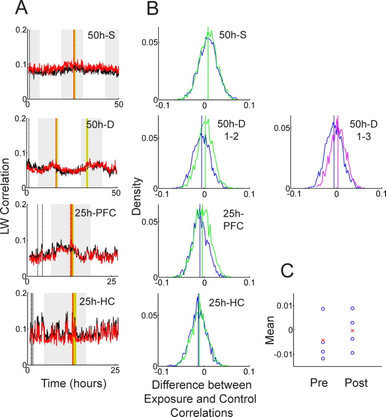
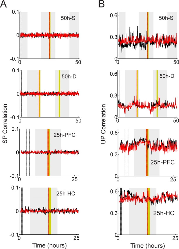
Template-matching analysis with the Louie–Wilson measure. A, Time evolution of exposure correlation (red) and control correlation (black) is calculated with the LW measure: from top to bottom, the 50 h recording with a single exposure (50 h S), the 50 h recording with dual exposures (50 h D), the 25 h recording from the medial prefrontal cortex (25 h PFC), and the 25 h recording from the hippocampus (25 h HC). Yellow and gray bands indicate the exposure epochs and the light-off periods, respectively. Red and black dashed lines indicate the timing of the five exposure and five control templates, respectively. B, Density distribution of the differences between exposure correlations and control correlations in the pre-exposure epoch (blue) compared with the postexposure epoch (green) is shown. For the 50 h D recording, the comparison between the first 16 h free-running epoch (blue) and the last 16 h free-running epoch (pink) is also presented (in the second row). Blue, green, and pink vertical lines represent the means of the corresponding distributions. C, Distribution of the mean values of the density distributions of pre-exposure (Pre) and postexposure (Post) epochs in B. Blue circles and red crosses represent each mean value and their mean, respectively.

Explained variance method.

Similar to the template-matching method, we start with the spike matrix of the whole recording data with N cells (rows) and T time bins (columns). The pre-exposure and postexposure epochs are divided into 15 min segments. The matrix segment of dimension N × M_PRE(1), with a typical bin-width of 250 ms and M_PRE(1) corresponding to 15 min just before the novel experience is taken as the first pre-exposure block PRE(1). The matrix segment of dimension N × M_EXP is taken from the novel experience epoch where M_EXP bins correspond to the waking portion of the active behavior (EXP) epoch. Finally, the matrix segment of dimension N × M_POST(1) just after novel experience, where M_POST(1) corresponds to 15 min, is taken as the first postexposure block POST(1). For each block, the pair-wise correlation matrix c_ij of all cell pairs from different tetrodes is calculated using the Pearson correlation coefficient:

where i and j represent the ith and jth row respectively, and x̄_i and x̄_j are the corresponding row means, defined as

Note that M in the above summation corresponds to either M_PRE(1), M_EXP, or M_POST(1), depending on the blocks. The resulting pair-wise correlations c_ij form a symmetric N × N matrix, C, with unit diagonal elements c_ij = 1. Three correlation matrices, C_PRE(1), C_EXP, and C_POST(1), one for each block, are created. Because these matrices are symmetric, only the lower off-diagonal elements are then rearranged into a vector and used in the following calculation. To evaluate the similarity between these three correlation matrices, we calculate the Pearson correlation coefficient between the blocks, obtaining R_{PRE(1), EXP}, R_{EXP, POST(1)}, and R_{PRE(1), POST(1)}. The coefficient between exposure and postexposure blocks, R_{EXP, POST(1)}, may, however, contain pre-existing effects from the pre-exposure epoch, PRE(1). Therefore, we calculate the partial correlation coefficient to subtract any pre-existing effect. The square of the partial correlation is called the explained variance (Kleinbaum et al., 1988) and is defined as follows:

To obtain a measure of how much of the EV can be generated by chance, we also calculate the reversed explained variance, EV_{EXP,PRE(1)|POST(1)}^REV. This reversed EV is defined by exchanging PRE(1) and POST(1) in the above EV formula, effectively reversing the role of time (Pennartz et al., 2004).

Finally, in our present analysis, we calculate multiple EVs corresponding to all of the postexposure blocks. To obtain means and error bars, an average of the EVs over all of the pre-exposure epochs is taken for each postexposure block. Suppose that the pre-exposure and postexposure epochs are first divided into K and H 15 min blocks, respectively. Explained variance of the hth postexposure block averaged over all of the K pre-exposure blocks, EV_{EXP, POST(h)|PRE}, is then calculated as follows:

Similarly, the corresponding reversed-EV is calculated as follows:

For the error bars, the SDs over the K pre-exposure blocks are taken.

Results

In this paper we use the term “reactivation” in the context of the explained variance analyses and the term “reverberation” in the context of the template-matching analyses. We consider both as forms of memory “replay” measured in different ways.

We also emphasize that all our methodological investigations in this paper refer to the Ribeiro et al. (2004) context and do not apply to the original study by Louie and Wilson (2001), which used different methods to obtain controls.

The Results section is organized as follows. To emphasize the proper application of the template-matching method, we first calculate the exposure and control correlations throughout the whole recording session, and compare them at the same time points. The results of this whole trace analysis are summarized in Figures 2 through 7. We then analyze the same data with a partial application of the template-matching method, as was used by Ribeiro et al. (2004), where the correlations at different time points are compared. The results of this potentially misleading partial trace analysis are depicted in Figures 8 and 9. We emphasize that the results obtained by the partial trace analysis (Fig. 8) show apparent “highly significant” reverberations, whereas the more detailed whole trace analysis (Figs. 2–7) of the same datasets shows no significant postexposure increase of reverberations. This example illustrates that improper, partial calculation of template-matching correlations may lead to erroneous conclusions. Additionally, to deepen our understanding of the template-matching method, the effect of normalization of mean firing rates is investigated in detail (Figs. 10, 11). Finally, the same recording data are analyzed by an independent statistical method, the explained variance method, and the result is presented in Figure 12.

Figure 7.

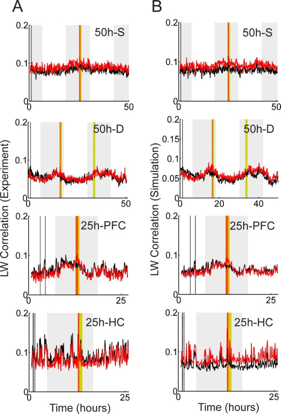
Comparison of the Louie–Wilson measure on experimental data and simulation data. A, The LW correlation on experimental data are shown. A bin width of 250 ms and a template length of 9 s are used in the template-matching calculation. B, The corresponding LW correlation on simulation data are shown. For the 50 h recordings, the mean firing rates of the experimental data are estimated at every 15 s using Gaussian windows with a width of 5 min. As for the 25 h recordings, the mean firing rates are estimated at every 3 s using Gaussian windows with a width of 1 min. Inhomogeneous Poisson spike trains are generated using these estimated mean firing rates, and the exposure and control templates are selected at the same time points as the experimental data. The LW correlation is then calculated using a bin width of 250 ms and a template length of 9 s.

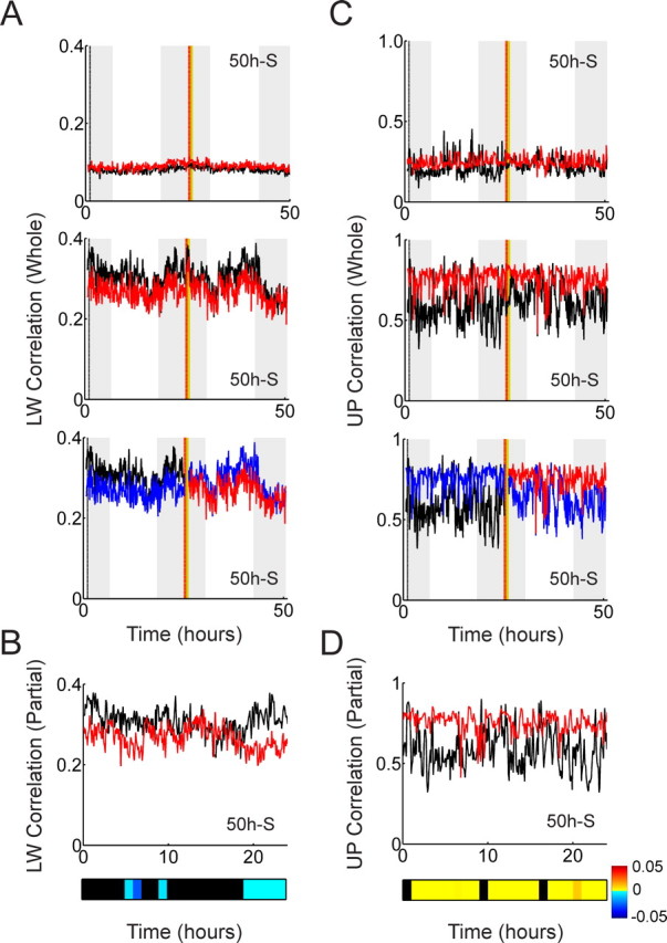
Figure 8.

Comparison of template-matching correlation between whole-trace and partial-trace calculation. A, Top, From left to right, the whole trace of the LW correlation of the 50 h recording with a single exposure, the 50 h recording with dual exposures (repeated twice for different Ribeiro-type decomposition later), the 25 h recording from prefrontal cortex, and the 25 h recording from hippocampus are shown, respectively. The parameter combinations, bin width of 250 ms and template length of 9 s, are used, and no significant long-lasting reverberation was observed. Bottom, The parts of the correlation curves that were not calculated by Ribeiro et al. (2004) are colored in blue. B, Deleting the blue curves and superimposing the red and black curves produces artificial long-lasting reverberation or anti-reverberation in four of five cases. Significance was assessed by Bonferroni test, and significant reverberation was depicted by a color scale ranges (0, 0.05) (yellow–red) and significant anti-reverberation by (−0.05, 0) (dark blue–light blue).

Figure 9.

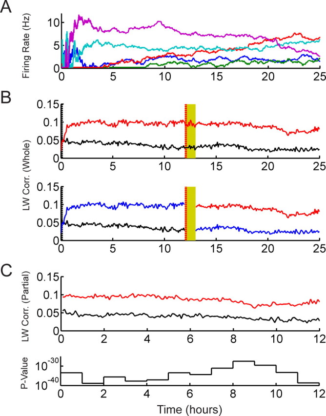
Simulation of transient modulation of mean firing rates and occurrence of systematically more reverberation than antireverberation. A, Typical time evolutions of the mean firing rates of five simulated model neurons. Each neuron generates an independent inhomogeneous Poisson spike train with mean firing rates modulated by a Brownian random walk. Transient instability is simulated by an exponential decay of the step-size of the walk, which results in large variability within the first ∼2 h, gradually reducing to a more stable regime with small remaining drift. Mean firing rates are bounded between 0.2 and 20 Hz. B, Top, The LW correlations of the whole simulation trace averaged over exposure (red) and control templates (black), respectively. Templates with a bin width of 250 ms and template length of 9 s are used. The vertical dashed red and black lines indicate the position of the exposure and control templates, respectively. The exposure templates systematically exhibit correlations higher than the control templates before and after the exposure epoch (yellow), and no significant long-lasting reverberation is observed. Occurrence of more reverberation than antireverberation is a robust feature regardless of simulation parameters such as initial step sizes, the decay constant of transient instability, and initial firing rates. Bottom, The parts of the correlation curves that were not calculated by Ribeiro et al. (2004) are colored in blue. C, Top, Removing the blue parts and superimposing the remaining red and black traces produces artificial long-lasting reverberation. Bottom, Apparent highly significant p values obtained by Bonferroni tests in successive 1 h segments.

Figure 3.

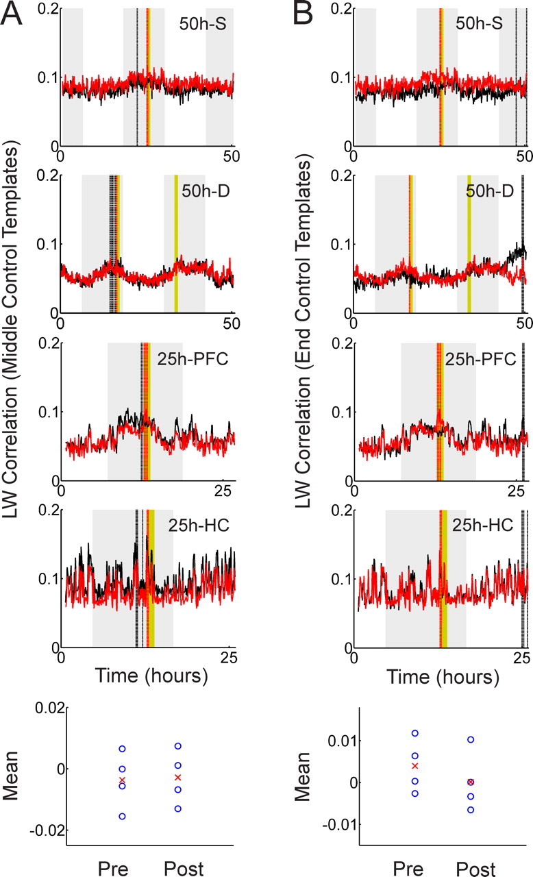
Template-matching analysis with the Louie–Wilson measure using middle and end control templates. A, LW correlation is calculated using five middle control templates that are taken just before exposure. B, LW correlation is calculated using five end templates near the end of the recording. The position of the control templates influences the relative relationship between exposure correlation and control correlation of the pre-epochs and postepochs.

Figure 4.

Parameter dependence of the Louie–Wilson measure. LW correlation for the hippocampal 25 h recording is calculated with three bin widths (50, 250, and 1000 ms) and three template lengths (1, 9, and 80 s).

Figure 5.

Effect of compression or expansion of memory-trace replay speed on the Louie–Wilson measure. The LW correlation was calculated using six different replay speeds. Different speed factors were obtained by changing the target matrix bin size (12.5 ms for 20 times, 16.7 ms for 15 times, 25 ms for 10 times, 50 ms for 5 times, 125 ms for 2 times, 250 ms for 1 time, and 500 ms for 0.5 times) with the template bin size fixed at 250 ms.

Figure 6.

Template-matching analysis with the standardized Pearson measure and the un-normalized Pearson measures. A, Template-matching analysis with the SP measure is shown; from top to bottom: the 50 h recording with a single exposure, the 50 h recording with dual exposures, the 25 h recording from the medial prefrontal cortex, and the 25 h recording from the hippocampus. B, The same data set was analyzed by the UP measure. No long-lasting reverberation was found with these alternate measures.

Figure 10.

Effect of the normalization of the Louie–Wilson measure on homogeneous Poisson spike trains. Normalized mean (solid) and variance (dashed) are plotted against the original mean and variance. Normalized mean and variance are bound between 0 and 1 (a solid horizontal line), and their crossover is obtained at ($\raisebox{1ex}{$(-1+\sqrt{5})$}\!\left/ \!\raisebox{-1ex}{$2$}\right.$. Areas above and below a diagonal line represents the enhanced and suppressed regions, respectively.

Figure 11.

Effect of smoothing on the Louie–Wilson measure and the un-normalized Pearson measures. A, Top, The time evolution of the LW measure of the 50 h recording with a single exposure (bin width, 250 ms; template length, 9 s) indicates no long-lasting reverberation. Middle, Gaussian window smoothing (σ = 1.5 s) makes control correlations higher than exposure correlations, but there is still no long-lasting reverberation. Bottom, The correlation curves that were not calculated by Ribeiro et al. (2004) are colored in blue. B, Superimposing the red and black curves on top of each other suggests (spurious) antireverberation. Significance was assessed by Bonferroni test. C, Top, The same data analyzed by the UP measure (bin width, 250 ms; template length, 9 s) indicate no long-lasting reverberation. Middle, Gaussian smoothing (σ = 1.5 s) increases both correlation values. Bottom, The correlation curves that were not calculated by Ribeiro et al. (2004) are colored in blue. D, Superimposing only the red and black curves suggests (spurious) reverberation. Significance was assessed by Bonferroni test. Note that partial analysis by LW and UP measures generates opposite observations.

Figure 12.

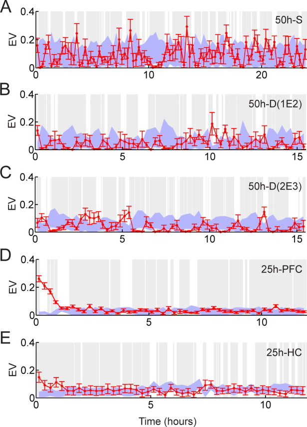
Analysis with explained variance method. A, The 50 h recording with a single exposure. B, The 50 h recording with dual exposures using the first 16 h free-running, the first exposure, and the second 16 h free-running epoch. C, The 50 h recording with dual exposures using the second 16 h free-running, the second exposure, and the last 16 h free-running epoch. D, The 25 h recording from the medial prefrontal cortex. E, The 25 h recording from the hippocampus. Using a 250 ms bin width and 15 min block size, explained variance is sequentially calculated over the whole postexposure epoch. Red dot and red error bars represent the mean and SDs of EV over pre-exposure blocks, respectively. The blue band shows the range (mean ± 1 SD) of the reversed EV. Gray and white regions correspond to scored rest and wake periods, respectively.

Long-lasting neuronal reverberation with the Louie–Wilson measure

We first discuss the template-matching analysis with the Louie–Wilson correlation measure. Figure 2A depicts the temporal evolution of the LW measure over the whole recording session. The top two panels, 50 h S and 50 h D, represent 50 h recordings with a single exposure and dual exposures, respectively, and the bottom two panels, 25 h PFC and 25 h HC, represent 25 h recordings from the prefrontal cortex and hippocampus, respectively. Red and black curves, corresponding to the exposure and control correlations, respectively, behave similarly throughout the recording. In other words, no significant divergence between red and black curves after the exposure epoch (yellow band) is observed, including during the dual exposure experiment (Fig. 2A, second panel). To assess significance, we calculated the difference between the red and black curves at every 30 s sampling point (control correlation was subtracted from exposure correlation). If long-lasting neuronal reverberation exists, the distribution of the differences should be significantly different in pre-exposure and postexposure epochs. Figure 2B depicts these distributions along with their mean values. Figure 2C shows individual mean values (blue circle, each corresponds to blue and green vertical lines in Fig. 2B) and their mean (red cross) in pre-exposure and postexposure epochs. The Wilcoxon matched-pairs signed rank test on these four pairs of mean values in pre-exposure and postexposure epochs gives p = 0.125, implying that no significant difference was detected.

Although the result of the Wilcoxon signed rank test was not significant, Figure 2C suggests a tendency that the means of the postexposure distributions are higher compared with those of pre-exposure (the red cross representing the mean in the postexposure epoch is higher than that in the pre-exposure epoch in Fig. 2C). In other words, a relative relationship between exposure correlation and control correlation is shifted in such a way that exposure correlation gets slightly higher after the exposure epoch. One might argue that more datasets could enhance this tendency to a statistically significant level if this small effect is caused by exposure to novel objects. An alternate explanation is that there might be a slow but systematic decay of template similarity over time and that this tendency is caused because exposure templates are located closer to the postexposure epoch than the control templates are.

To answer this question, we recalculated the correlations using control templates taken just before the exposure epoch and from the end of recording respectively. If the effect is caused by long-lasting reverberation, the relative relationship in Figure 2C should not change when varying the position of the control templates. If the effect is caused by different relative distances between templates and target matrices, however, “middle” control templates will produce almost equal means and “end” control templates will reverse the tendency in Figure 2C. Figure 3, A and B, shows the temporal evolution of correlations for middle control templates and end control templates, respectively. Note that the exposure correlations (red curves) are identical in Figure 2A and Figure 3, A and B, but the control correlations (black curves) vary because of different control templates. The corresponding individual mean values (blue circles) and their mean (red crosses) of pre-exposure and postexposure distributions are shown in the bottom panels of Figure 3, A and B. In both cases, the difference is not significant (The Wilcoxon signed rank test for middle and end control templates gives p = 0.625 and p = 0.125, respectively), but the relative relationships of the means are affected by the position of the control templates. The small positive tendency vanishes for middle control templates and reverses for control templates taken from the end. This leads to the conclusion that the small positive tendency observed in Figure 2C is not attributable to long-lasting neuronal reverberation but to the fact that exposure templates are located closer to the postexposure epoch than the control templates are.

At this point we would like to emphasize again that the figures depicting the time evolution of correlations in this study (Fig. 2A) and the corresponding figures in the study by Ribeiro et al. (2004) (their Fig. 2b) are constructed differently. In the study by Ribeiro et al. (2004), the control correlations are calculated for only the first half of the recording session (pre-exposure) and the exposure correlations for only the second half (postexposure). The two partial time series are then superimposed and horizontally aligned such that the room-light on/off cycles match. In contrast, the Figure 2A and Figure 3, A and B, in the present study depict the full time series of both control and exposure correlations over the entire recording sessions, and therefore no realignment is required. Ribeiro et al. (2004) compare correlations from different time points on the same time-axis, whereas our study consistently compares correlation values at the same time points. In light of the above observations, this difference in procedure leads to a very important consequence investigated in detail in a later section.

Parameter dependence of long-lasting neuronal reverberation with the Louie–Wilson measure

We have not found statistically significant long-lasting reverberation using the same template parameters as Ribeiro et al. (2004), where the bin width is 250 ms and the template length is 9 s. This does not exclude, however, the possibility that long-lasting reverberation could be detected with different template parameters. We, therefore, conducted an extensive parameter search varying the bin width from 50 to 1000 ms and the template length from 1 to 80 s.

Figure 4 shows the parameter dependence of the LW correlations obtained from the 25 h recording from hippocampal CA1 (25 h HC, 48 cells). In the top left panel the templates have 1600 columns (50 ms bins and 80 s template length), whereas in the bottom right panel the templates have only 1 column (1 s bin and 1 s template length). Note that the middle panel corresponds to the parameters by Ribeiro et al. (2004). Note also that the bottom right panel corresponds to the state vector-matching method (McNaughton, 1998), which is considered a special one-bin case of the more general template-matching method. The state vector method assesses the reoccurrence of a specific pattern of mean firing rates across the neurons, which can be considered as one specific form of memory trace reactivation. There is a tendency that correlation values increase with the size of bin width. This occurs because more spikes are considered to be “synchronous” under wider bin width. As for the relationship between correlation values and template length, we also notice that the correlation becomes smaller with an increase of template length. This observation implies that the spatiotemporal patterns induced by novel and familiar experiences do not last very long. Another interesting observation is that the relative relationship between the exposure correlation and the control correlation changes for certain parameter combinations; for example, the bottom right panel (1 s bin and 1 s template length) and the middle right panel (1 s bin and 9 s template length) show higher control correlation than exposure correlation. As demonstrated in a later section, this kind of change may be caused by normalization of the mean firing rate in the LW measure.

Although correlation values differ depending on parameter combinations, Figure 4 clearly shows that the overall exposure and control LW correlations look very similar in all of the parameter ranges, indicating that there is no obvious long-lasting reverberation in these data. The analyses of the three other recording sessions show similar properties (for data, see supplemental Figs. 7–9, available at www.jneurosci.org as supplemental material). No significant p values (p < 0.05) were obtained by the Wilcoxon signed rank test on these four recordings, confirming that no significant long-lasting reverberation is detected at any parameter combination.

Effect of time compression or expansion on the Louie–Wilson measure

Memory-trace replay may occur with temporal evolution rates that differ from that observed during the behavioral episodes (Skaggs and McNaughton, 1996; Nadasdy et al., 1999; Louie and Wilson, 2001; Lee and Wilson, 2002). To investigate whether long-lasting reverberation can be detected at a different playback speed, we calculated the LW correlation with different speed factors: 20, 15, 10, 5, 2, and 0.5× compression rate. Figure 5 shows the time evolution of the LW correlation with different speed factors, including a default, no compression case (1×). Figure 5 clearly shows that the exposure correlation and the control correlation look very similar. No significant long-lasting neuronal reverberation was detected in any parameter range by the Wilcoxon signed rank test.

Long-lasting neuronal reverberation with standardized Pearson's measure and un-normalized Pearson's measure

The template-matching method aims to assess similarity between two matrices. It is generally known, however, that the Pearson correlation coefficient, which serves as a basis for the template-matching analysis here, is affected by both fine spike-timing relations among neurons and mean firing rate (Ito and Tsuji, 2000). In principle, the contributions from the fine spike-timing structures can be reduced by smoothing along the rows of the matrices, and the mean firing rate differences can be reduced by judicious normalization of each row by its row-mean, row-variance, or related quantities. Thus, the similarity of spatiotemporal patterns between a template and a target matrix is dependent on how fine spike-timing relations and mean firing rate are treated in the correlation measure. Our failure to find significant long-lasting reverberation with the LW correlation measure, therefore, does not exclude the possibility that it may be detected by other correlation measures with different smoothing and/or normalization. Because Ribeiro et al. (2004) did not use smoothing in their analysis, we focus in this study on the effect of normalization.

In the Louie–Wilson measure, which was used by Ribeiro et al. (2004) and was also used in our investigation so far, each row is normalized by its root mean square amplitude. This normalization dramatically reduces the contributions caused by mean firing rate differences among neurons, but does not fully eliminate it. Therefore, the LW measure is affected not only by the fine spike-timing structures but also the remaining mean firing rate differences. If the two factors are treated differently from the LW measure, does long-lasting reverberation emerge from our data sets?

To answer this question, we analyzed the data with the SP measure as well as the UP measure. The SP measure normalizes each row by subtracting its row mean and dividing by its SD. In the resulting normalized matrix, each row has zero mean and unit variance, implying that only fine spike-timing structure remains in the matrices; mean firing rate differences are fully suppressed. On the other extreme, the UP measure does not involve any row normalization at all. This measure is more strongly influenced by mean firing rate differences than the LW measure. Figure 6, A and B, shows the results from the SP and UP measures respectively. The correlations in Figure 6A turn out to be almost flat, fluctuating around zero throughout the recording. This indicates that the fine spike-timing structure has almost no contribution to template-matching correlations, and there is no obvious sign of long-lasting neuronal reverberation (p = 0.625 by the Wilcoxon signed rank test of the means in pre-exposure and postexposure epochs). As for the UP measure depicted in Figure 6B, both the correlation levels and variability become larger than those of the LW measure, indicating that the mean firing rate fluctuations contribute much more strongly. However, the Wilcoxon signed rank test gives p = 0.625, suggesting that no significant long-lasting reverberation is detected.

Long-lasting reverberation investigated by inhomogeneous Poisson spike trains

The observations in the previous section indicate that the mean firing rate difference, and not fine spike-timing relationships, is the main contributor to the correlation measures in this novel experience protocol. This is clearly contrasted by the work of Louie and Wilson (2001) in which the rat ran on the familiar track repeatedly and therefore temporally structured multineuronal spike patterns were observed. They successfully detected a significant similarity of these temporal spike patterns with LW measures. In contrast, in the novel experience task of the present study, there is no imposed repetitive temporal order during the exposure epoch, because the rat was allowed to explore the novel objects freely. Therefore, it seems to make sense that the mean firing rate difference but not fine spike-timing relationships is the main contributor to the correlation measure.

To support this view further, we calculated the LW measure on artificial spike trains without fine temporal structure. The artificial spike trains were generated as inhomogeneous Poisson spike trains with variable mean firing rates. The slowly changing mean firing rates were estimated from experimental data by smoothing with a Gaussian window of 1–5 min. By construction, the artificial spike trains have slow fluctuations of mean firing rate but do not have any fine spike structure within the template length. Figures 7, A and B, shows the LW correlation calculated with the experimental data and with the artificially generated inhomogeneous Poisson spike trains, respectively. The good match between Figure 7A and B, supports the conclusion that slow changes of mean firing rates account for most of the LW correlation amplitude.

Taking all of the observations from Figures 2 through 7 together, we conclude that no statistically significant long-lasting neuronal reverberation of novel experience is detected in the present recording by the template-matching method, neither with the Louie–Wilson measure, standardized Pearson measure, nor the un-normalized Pearson measure. We also investigated the compression or expansion of memory-trace replay speed, but did not detect any significant long-lasting reverberation. These investigations further indicate that, in this novel experience protocol, slow fluctuations of mean firing rates contribute primarily to the correlation amplitude whereas the fine temporal structure of spike trains has almost zero effect. This fact was also verified by a simulation using inhomogeneous Poisson spike trains.

Partial calculation of template-matching correlations may lead to incorrect conclusions

One may speculate that the disagreement between the results by Ribeiro et al. (2004) and our observations is attributable to recording from different brain areas. Although it is true that recording sites do not overlap exactly between the two studies, a good chance of detecting long-lasting reverberation was expected, especially in the 25 h recordings from the local areas, because the hippocampus is an area where Ribeiro et al. (2004) found significant long-lasting reverberation and the medial prefrontal cortex is an area in which reactivation of familiar memory traces has been found (Euston et al., 2005) and also receives projections from the hippocampus (Ferino et al., 1987). However, because the recording sites are not exactly the same, the present study does not directly contradict the original results obtained by Ribeiro et al. (2004), but rather reflects an inconsistency between these independent observations.

There is, however, one crucial difference between the two studies. As was pointed out in the previous section, in the study by Ribeiro et al. (2004), control correlations were calculated only during the pre-exposure epoch and exposure correlations were calculated only during the postexposure epoch. These separately calculated correlation curves were aligned such that the room-light on/off cycles matched, and displayed on top of each other. A significant and sustained difference between these two curves was interpreted as long-lasting neuronal reverberation [for example, see Ribeiro et al. (2004), their Fig. 2b]. The authors, however, did not provide any information on the temporal evolution of the exposure correlations during the pre-exposure epoch, nor on the temporal evolution of the control correlations during the postexposure epoch. In contrast, we studied both exposure and control correlations throughout the whole recording session. No realignment was performed. Only if the difference between exposure and control correlations at identical time points was significantly larger after exposure, would we claim long-lasting neuronal reverberation (Fig. 1).

The underlying assumption behind the partial comparison performed by Ribeiro et al. (2004) is that a correlation evolution, similar to the artificial example in the lower panel of Figure 1, took place. There, both exposure and control correlation curves are similar in the pre-exposure epoch, but exposure correlation is significantly enhanced because of reactivation, and it is sustained for many hours. There is, however, no guarantee that this kind of time evolution took place. For example, the top panels of Figure 8A depict the same traces as the four panels of Figure 2A (a trace from the dual exposure 50 h recording was repeated twice for different reconstruction purposes later), showing the time evolution of the LW correlations of the four recordings. It was discussed above that we do not observe significant long-lasting reverberation in these recordings. In the bottom panels of Figure 8A, those parts of the exposure and control correlations that were not calculated by Ribeiro et al. (2004) are colored in blue. By removing the blue curves and superimposing the remaining control correlations (black curve) and exposure correlations (red curve), we obtain Figure 8B. Following methods of Ribeiro et al. (2004), significance of reverberation and antireverberation was assessed by a Bonferroni comparison of five paired t tests between each exposure correlation and template-averaged control correlation. Control correlations were averaged over five templates to avoid ambiguity of pairing five exposure correlations and five control correlations. Significance was assessed in successive 1 h segments, and the sum of individual p values is depicted using a color bar with a color scale in the ranges (0, 0.05) (yellow-red) for reverberation and (−0.05, 0) (dark blue–light blue) for antireverberation, whereas black denotes nonsignificance (p > 0.05). Given the partial traces, we could now claim “apparently significant” long-lasting reverberation or long-lasting antireverberation except for the single exposure 50 h recording where no significant differences were detected. Furthermore, if improper correlation comparison drives apparent reverberation, one would expect to see as much antireverberation as reverberation. If we count the number of blocks that show significant reverberation or antireverberation in the present analysis, we obtained 12 and 13 blocks for reverberation and antireverberation, respectively. This observation supports the idea that these reverberations and antireverberations are artifacts generated by partial comparison of correlation traces, which, in the present case, leads to incorrect conclusions.

As demonstrated here, a partial calculation of template-matching correlation is not sufficient to detect long-lasting reverberation. Slow systematic drift in mean firing rate, which was shown to be the main contributor to the correlation in this novel experience task, may create artifacts and lead to incorrect conclusions. To resolve the inconsistency between Ribeiro et al. (2004) and the present study, an analysis of the whole recording trace of their data are necessary.

Transient instabilities at the beginning of recordings can systematically produce more apparent reverberation than antireverberation

If a slow, systematic change in mean firing rates creates erroneous reverberation and antireverberation in partial correlation calculations, it is important to assess the relationship between mean firing rate modulations and the induced apparent reverberation/antireverberation in a simulation study. We considered two kinds of modulations of mean firing rates: one where the change is oscillatory with a constant wavelength throughout the recording whereas in the other the changes occur randomly and transiently. To investigate the former, we conducted a simulation with artificial neurons, each generating an inhomogeneous Poisson spike-train in which the mean firing rates vary according to sinusoidal waves with constant wavelengths and random phases. By partial correlation comparison, we find both reverberations and antireverberations, which are related to the speed of modulation (wavelengths) of the mean firing rates. A detailed report of this simulation study is presented in the supplemental information (available at www.jneurosci.org as supplemental material).

To investigate the latter case, in which the modulation of mean firing rates occurs randomly and transiently, we simulated a scenario where the instability is larger in the beginning of the recording and reduces to a slow remaining drift throughout the rest of the recording. This scenario is plausible in the case where an initially sizeable instability is induced by experimental setup manipulations, such as attaching the recording cables to the head stage, and a subsequently more agitated behavior of the animal. Such initial instabilities may systematically decrease with time when the animal settles into its routine behavior and/or electrodes perturbed by the attachment of the headstage stabilize once again in the brain.

We generated a 25 h dataset with 50 simple model neurons, each producing an inhomogeneous Poisson spike train with time-dependent mean firing rates, which were independently modulated by a Brownian random walk restricted to a range between 0.2 and 20 Hz. The step-size of the random walk was set to a large value at the beginning of the recording and was decreased exponentially with a decay time constant of 1 h to a very small step-size (for details, see supplemental text, available at www.jneurosci.org as supplemental material). Figure 9A depicts typical traces of the mean firing rates versus time of five model neurons. Note the large instabilities in the first ∼2 h, which gradually reduce to a slow drift because of the small random walk step-size throughout the remaining simulation. The traces of all 50 model neurons are shown in supplemental Figure 11, available at www.jneurosci.org as supplemental material.

A template-matching analysis using the Louie–Wilson measure was performed using five control templates from the beginning of the simulation and five exposure templates from the exposure epochs, both groups with 90 s intertemplate distances. Template bin width and length were set to 250 ms and 9 s, respectively. The top panel of Figure 9B shows the Louie–Wilson correlations calculated over the whole recording trace. It is clearly seen that exposure and control correlations are roughly parallel throughout the recording except at the very beginning where the mean firing rates vary strongly. In other words, no long-lasting reverberation is observed with the whole trace calculation, but rather a systematic offset between exposure and control template correlations is maintained throughout the pre-exposure and postexposure epochs. The blue curves in the bottom panel of Figure 9B indicate the parts that were not calculated by Ribeiro et al. (2004). By removing the blue curves and superimposing the remaining control correlations (black curve) and exposure correlations (red curve), we obtain the data in the top panel of Figure 9C. Similar to the previous section, we now observe apparent long-lasting reverberation. Again, the significance is assessed by Bonferroni tests on successive 1 h segments, and the corresponding p values, ranging from ∼10⁻²⁵ to 10⁻⁴⁰, are provided in the bottom panel of Figure 9C. Combination of transient modulation of mean firing rates and the partial correlation comparison gives a highly significant result, which is, however, artificially induced by partial calculation of the template-matching correlation.

We note that the qualitative features of this particular example are robust when the parameters of the simulations are varied, whereas the quantitative amount of the offsets varies nonlinearly with different parameter choices as well as the time-separation between templates. One critically important and robust observation in all simulations of this scenario is that systematically many more reverberations are obtained than antireverberations. This is in clear contrast to the case in the previous section where our experimental data were analyzed by partial comparison and also to the former simulation with sinusoidal waves in the mean firing rates (detailed in the supplemental text, available at www.jneurosci.org as supplemental material). Both of these previous investigations gave an almost equal number of apparent reverberations and anti-reverberations.

In the present transient instability simulation, the control templates are taken when the mean firing rates vary strongly (the first ∼2 h in Fig. 9A),. This makes the control and target matrices quickly dissimilar with increasing time, resulting in relatively low values of template-matching correlations. However, because the exposure templates are taken when the cells are more stable, the similarities between the template and target matrices are consistently stronger, giving relatively high template-matching correlation values. Therefore, partial correlation calculation gives many more cases of reverberation than antireverberation in this scenario, where the control templates are taken during a period of greater instability at the beginning of a recording and the exposure templates are taken from a period when the cells have more stable mean firing rates.

In the study by Ribeiro et al. (2004) we notice that their Figure 2 shows only reverberations but no antireverberations, and that their Figure 3 has many more reverberations than antireverberations. In other words, contrary to our experiments, where almost equal number of reverberations and antireverberations are obtained (Fig. 8B), they observed systematically more reverberation than anti-reverberation in their partial trace analysis. The foregoing simulation provides at least a plausible scenario by which these differences may have come about. If this conjecture is correct, then reanalysis of the data of Ribeiro et al. (2004) using the whole-trace calculation procedure might produce results qualitatively similar to Figure 9B, which would indicate that the observed difference between exposure and control traces is present equally before and after the exposure epoch and therefore has no causal connection to the novel experience.

Normalization of template-correlation measures affects detection of reverberation

The effect of normalization on the template-matching method is not as simple as it may appear. For example, the normalization in the LW measure leads to a nonlinear contribution from mean firing rate differences among neurons. To understand the effect of this normalization more clearly, we illustrate how simple spike trains are transformed by the normalization of the LW measure. Suppose that spike trains in the template matrix and in the target matrix are approximated by homogeneous Poisson spike trains. Both the mean and variance of ith row is written as λ_i. After the normalization of the LW measure (i.e., the mean firing rate of each row is divided by its root mean square amplitude), the transformed spike train has mean and variance $\sqrt{\raisebox{1ex}{$1$}\!\left/ \!\raisebox{-1ex}{$1+\raisebox{1ex}{$1$}\!\left/ \!\raisebox{-1ex}{${\lambda }_i$}\right.$}\right.}$ and $\raisebox{1ex}{$1$}\!\left/ \!\raisebox{-1ex}{$1+{\lambda }_i$}\right.$), respectively. Figure 10 shows how this normalization scales with respect to the original mean and variance, λ_i. Solid and dashed lines represent mean and variance, respectively. The normalization assures that both firing rate and variance are restricted to values <1, indicating that the mean firing rate difference among neurons is dramatically reduced. However, because the transformation is nonlinear, the contributions of rows with the original mean (and also the original variance) less than ($\raisebox{1ex}{$(-1+\sqrt{5})$}\!\left/ \!\raisebox{-1ex}{$2$}\right.$ are enhanced, whereas those from rows with the original mean (and also the original variance) greater than ($\raisebox{1ex}{$(-1+\sqrt{5})$}\!\left/ \!\raisebox{-1ex}{$2$}\right.$ are suppressed. In other words, the contribution from the neurons whose mean firing rate is less than ($\raisebox{1ex}{$(-1+\sqrt{5})$}\!\left/ \!\raisebox{-1ex}{$2$}\right.$ is enhanced whereas the contribution from the neurons whose mean firing rate is greater than ($\raisebox{1ex}{$(-1+\sqrt{5})$}\!\left/ \!\raisebox{-1ex}{$2$}\right.$ is suppressed. This simple example shows that even in this basic case, the effect of the normalization in the LW measure is quite complicated. Furthermore, simultaneous application of normalization of mean firing rate and smoothing of bins makes the situation even more complicated.

Although a detailed characterization of template correlation measures is beyond the scope of this paper, we demonstrate how the LW and UP measures may lead to different conclusions, especially if only partial trace correlations are calculated. Note that the only difference between these two measures is that the former normalizes the mean firing rate of each row by its root mean square amplitude whereas the latter does not involve any row normalization.

The first panels in Figure 11, A and C, show the time evolution of correlations from the 50 h recording with a single exposure (50 h S), calculated with the LW measure (Fig. 11A) and the UP measure (Fig. 11C) with a bin width of 250 ms and a template length of 9 s. As expected, the result for the UP measure shows higher correlation amplitudes and larger variability than the LW measure because of stronger contribution from mean firing rate differences among neurons. However, no long-lasting reverberation is observed by the whole-trace calculation of both measures. The second panels in Figure 11, A and C, show the analyses of the same data with smoothing of the bin contents along each row (Gaussian window of 1.5 s), thereby reducing the contributions from fine spike-timing structures. Interestingly, for the LW measure the relationship between the amplitude levels of the control correlations (black curve) and exposure correlations (red curve) is reversed, whereas for the UP measure it stays in the same order. This disproportional change in amplitudes is caused by the nonlinear normalization of mean firing rates in the LW measure. Note, however, that long-lasting reverberation is still not observed by the whole-trace calculation of both measures. Note also that this kind of disproportional change was not apparent in the other three recordings, and that it is difficult to predict when it occurs, because of the nonlinearity of the normalization. In the third panels of Figure 11, A and C, those correlations that were not calculated by Ribeiro et al. (2004) are colored in blue. By removing the blue curves in the third panels of Figure 11, A and C, and superimposing the remaining red and black curves, the data in Figure 11, B and D, are created. Figure 11, B and D, suggests completely opposite results, antireverberation by the LW measure and reverberation by the UP measure. Thus, our conclusions from the partial calculation of correlation would depend on the choice of normalization and smoothing. By calculating the correlations of the whole recording (Fig. 11A,C, second panels), we can avoid such contradicting and misleading conclusions.

Long-lasting neuronal reactivation by the explained-variance method

Although statistically significant long-lasting neuronal reverberation is not confirmed by the TM method, there may be a trace of memory reactivation that can be detected by different statistical methods. For this purpose, we analyzed the same data using the EV method (Kudrimoti et al., 1999). The two methods are quite different in their construction, and therefore may give different results. Several important differences include how multineuronal correlation, temporal correlation and pre-existing correlations are treated, respectively. As for the spatial dimension, the TM method takes all of the available neurons into the matrix at once, whereas the EV method uses pair-wise correlations of all available neuron pairs. As for the temporal dimension, the TM method implies a shorter time scale which is determined by template length [9 s in a study by Ribeiro et al. (2004) and up to a couple of minutes in a study by Louie and Wilson (2001)], whereas the EV method usually averages over a longer time scale, typically 10–15 min. It should be also pointed out that the EV method is unaffected by any permutation of columns. Finally, the TM method does not correct for pre-existing correlations whereas the EV method uses the partial correlation coefficient to subtract pre-existing effects. In summary, the TM method is designed to detect similarity between a template and a target matrix in terms of spatiotemporal patterns of all available neurons on a short time scale [9 s in a study by Ribeiro et al., (2004)]. In contrast, the EV method is designed to detect enhanced similarity between behavior and postbehavior cell–cell correlation matrices, obtained on longer time scales (15 min) by subtracting pre-existing pair-wise correlations between behavior and pre-behavior epochs.

To assess significance, the EV method compares the EV values with reversed-EV values (Pennartz et al., 2004). The latter are defined by exchanging pre-exposure and postexposure epochs in the explained variance formula, thereby estimating the similarity between exposure and pre-exposure epochs. Because reversed-EV measures pre-existing correlations, it indicates how much of explained variance can be generated by chance. Note that, by construction, EV and reversed-EV at the same time points are not independent but slightly anticorrelated, leading to a dip in reversed-EV whenever the EV peaks. Therefore, each EV value should not only be compared with the corresponding reversed-EV in the same segment, but in a wider neighborhood of the segment.

Figure 12 shows the results of the EV analyses. The first panel represents the 50 h recording with a single exposure epoch (50 h S), the second and third panels represent the 50 h recording with dual exposure epochs [split into 2 datasets, 50 h D(1E2) and 50 h D(2E3)], each consisting of pre-exposure, exposure, and postexposure), the fourth and fifth panels depict the two 25 h recordings from the medial prefrontal cortex (25 h PFC) and hippocampus (25 h HC), respectively. The abscissa shows elapsed time in the postexposure epoch and the EV values (red dots) are shown with its SDs (red error bars) for every 15 min segment. The blue band represents the range (means ± SD) of the reversed-EV values, and white and gray bands represent waking and sleep, respectively. Note the difference that white and gray bands in the figures for the TM method represent the room light on/off cycle. In the first three panels of Figure 12, most of the EV and reversed-EV values fluctuate between 0 and 0.25, overlapping throughout the postexposure epoch. Thus, no reactivation can be claimed for either 50 h recording where the cells are distributed over many brain areas. In the 25 h PFC recording, explained variance in the first hour (the first four red data points) is clearly higher than the blue band of reversed-EV [exponential decay time constant of EV, τ = 39 min; 95% confidence interval, (32.9, 45.0)], indicating that short-lasting memory-trace reactivation caused by novel experience is detected in the medial prefrontal cortex. In the 25 h HC recording, the first EV data point, corresponding to the first 15 min of postexposure epoch, is ∼2 SDs higher than the blue band in its neighborhood [exponential decay time constant of EV, τ = 37 min; 95% confidence interval, (15.5, 58.3)]. This indicates that short-lasting memory-trace reactivation caused by novel experience is also present in the hippocampal CA1 area.

In summary, using the EV method, we detected clear short-lasting memory-trace reactivation of novel experience in the medial prefrontal cortex. We also found memory-trace reactivation of novel experience in the hippocampal CA1 area, which is consistent with a previous study (Kudrimoti et al., 1999). These memory-trace reactivations are not long-lasting however; they decay with time constants on the order of 40 min.

Discussion

Hippocampus-dependent memory consolidation in rodents typically requires several weeks (Riedel et al., 1999; Shimizu et al., 2000). The trace reactivation theory postulates that, during this time, repeated reactivation of stored traces orchestrates the gradual rearrangement of corticocortical connections that ultimately sustain the memory in a hippocampus-independent form; yet until recently, there was only scant neurophysiological evidence for reactivation lasting >1–2 h. The replay of memory-traces of familiar experiences often decays to undetectable levels in ∼1 h, although it is not clear if replay of novel experience is comparable in either magnitude or time course. Thus, the report by Ribeiro et al. (2004) describing memory trace reverberation lasting several days potentially represents a critical contribution to the field. As such, the phenomenon requires independent verification and additional study.

The present study demonstrates that different analysis methods may lead to very different, apparently conflicting conclusions. Thus, apart from the presentation and interpretation of new data, a constructive discussion about “methodology,” as attempted in this study, is also warranted.

Four continuous recordings lasting from 25 to 50 h were conducted using a 240-electrode drive that covers a large region of the rodent brain, and a 12-tetrode drive that covers local areas. To emphasize the proper application of the template-matching method, we first calculated the correlations throughout the whole recording session using the Louie–Wilson measure, but extensive investigation, including different parameters (bin width and template length) and different replay speeds, did not confirm long-lasting reverberation. The template-matching analyses using two other algorithms, the standardized Pearson measure and un-normalized Pearson measure, also failed to confirm long-lasting reverberation. By comparing the three different measures, we demonstrated that the mean firing rate difference among neurons, but not the fine spike-timing structure, was the main contributor to the template-matching correlation in the present study. This interpretation was further supported by computer simulations using inhomogeneous Poisson spike trains.

We investigated the apparent inconsistency between the results of Ribeiro et al. (2004) and our observations, and showed that a partial calculation of template-matching correlations, such as used by Ribeiro et al. (2004), may lead to erroneous conclusions. Although our data also showed apparently significant reverberations if a partial comparison is used, the whole trace calculations suggest that there was no long-lasting reverberation causally connected to the novel experience; reverberations and antireverberations appear as likely before as after the exposure. A simulation study with transient instability in mean firing rates, showed that such a scenario can systematically induce many more apparent reverberations than antireverberations in partial comparisons, as reported by Ribeiro et al. (2004). Additionally, detailed study of template-matching measures elucidated that the Louie–Wilson normalization of mean firing rates and smoothing affect correlation values nonlinearly.

We did not detect long-lasting reverberation either when averaging across templates as done by Ribeiro et al. (2004) or using individual templates recorded during contact with specific objects (data not shown). In contrast, using the explained variance method (Kudrimoti et al., 1999), short-lasting reactivation of novel experience was detected in the medial prefrontal cortex and in the hippocampus, both for the data from the entire behavioral sequence and for subsets of the data associated with exploration of specific objects (data not shown), although the data were not sufficient to detect object-specific effects. These observations are consistent with a previous study that reported short-lasting reactivation of novel experience during slow-wave sleep in the hippocampus (Kudrimoti et al., 1999).

One might argue that we did not find long-lasting reverberation because our recording sites were not directly related to somatosensory areas. We do not have enough data to clarify this point, although the difference in recording areas may have contributed; however, the fact that we also find apparently significant reverberation in our data by partial trace comparison suggests that the partial versus whole calculation of template-matching correlations is a primary issue here.

According to clinical observations in humans (Squire et al., 1993; Teng and Squire, 1999) and lesion studies in animals (Winocur, 1990; Zola-Morgan and Squire, 1990; Kim and Fanselow, 1992; Kim et al., 1995; Takehara et al., 2003), the hippocampus seems to play an important role in the initial stage of encoding, but the memory may be gradually consolidated in the neocortex and eventually become independent of the hippocampus (Scoville and Milner, 1957; Zola-Morgan and Squire, 1993) (but see Nadel and Moscovitch, 1997). It has been conjectured that the spontaneous reactivation of memory-traces in the hippocampus during subsequent sleep may orchestrate memory consolidation in neocortical circuits (Marr, 1971; Buzsaki, 1989; Chrobak and Buzsaki, 1994; McClelland et al., 1995; Hoffman and McNaughton, 2002; Battaglia et al., 2004). Our observations that both the hippocampus and medial prefrontal cortex can show short-term memory-trace reactivation after a novel experience are consistent with this conjecture. They may also provide some indication that both areas are coactivated in the initial encoding stage, although a simultaneous recording from the prefrontal cortex and hippocampus is necessary for additional support of this hypothesis.

Reactivation may occur in multiple waves. A study by Ramirez-Amaya et al. (2005) revealed two waves of Arc (Lyford et al., 1995) protein expression in the hippocampus and parietal cortex after novel experience. Because Arc protein appears to regulate AMPA receptor trafficking, it may play an important role in synaptic plasticity. The initial expression of Arc protein is observed from 30 min to 2 h after novel experience whereas the secondary expression occurs between 8 and 24 h after the experience. In the second wave, however, significantly fewer cells expressed Arc protein than in the first wave. If memory-trace reactivation and Arc protein expression are positively correlated, the study suggests that there may be a second wave of weak memory-trace reactivation between 8 and 24 h after novel experience that engages fewer cells; however, limitation in both the ability to record from a very large neuronal population and current statistical methods, including template matching and explained variance, limit our ability to detect such a subtle reactivation.

In general, all statistical methods for the detection of memory trace reactivation are sensitive not only to the number of neurons included in the analysis but also to which neurons. For example, consider two independent (i.e., not synaptically coupled) pools of neurons, each driven by the sensory and behavioral contingencies of the to-be-remembered experience. Suppose one subgroup of neurons contains associatively modifiable recurrent connections and, hence, exhibits attractor dynamics, whereas the other group contains no such connections. The former group might thus exhibit reactivation, whereas the latter would not. Inclusion of the latter cells in the analysis would dilute the population of reactivating neurons and possibly obscure actual reactivation. Therefore, in general, it is not necessarily the case that more recorded neurons will increase the power to detect reactivation, especially when the recorded neurons come from widespread brain regions. Disparity of the number of neurons between the study by Ribeiro et al. (2004), in which 59–159 neurons per animal were included in the analysis, and the present study, in which 31–48 neurons per animal were included, may affect the results of the template-matching method, but additional comparison is difficult at this point.

For the present study, the concern that too few neurons were sampled would more directly apply to the distributed recording (rat 1), because it included a relatively low number of somatosensory, hippocampal, caudate–putamen, and thalamic neurons. We examined reverberation using only cortical, hippocampal, or caudate–putamen neurons (we could not examine the thalamic case because there were too few units), but apparent reverberation was not detected in any of these subgroups. However, the two local recordings (rats 2 and 3), in which the prefrontal cortex and hippocampus were targeted, respectively, can be considered to have included a substantial portion of neurons in or connected to the “attractor” subgroup because a short-lasting reactivation was detected by the explained variance method in two animals. Finally, for these two local recordings, an analysis using partial groups of neurons such as pyramidal cells only and interneurons only was conducted to investigate if partial populations of neurons give clearer signals, but again, the data are insufficient to allow any inferences.

In the application of the template-matching method, a fundamental problem is how to implement the proper controls. One issue is the partial- versus whole-trace comparison discussed in the present study. In addition, potential artifacts may arise from mean firing rate fluctuations. This issue was also addressed in the original study by Louie and Wilson (2001), in which different bootstrapped shuffling procedures were proposed to obtain the proper controls for these artifacts.

Which part of the biologically relevant information is coded by the mean firing rate fluctuations among neurons and which part by the fine spike-timing structure is a common issue. In most situations there are no good criteria for choosing an “optimal” template-matching measure; should one use the UP, LW, SP, or any other thinkable measure? Because each of these measures emphasizes a different aspect of the data, it is illuminating to study several measures in parallel; however, independent of the choice of measure, the key issue in template matching is the proper application of controls, such as a full trace comparison and bootstrapped shuffling methods as used by Louie and Wilson (2001).

In summary, although our observations do not directly contradict the original results by Ribeiro et al. (2004), our present methodological studies raise reasonable doubt about their conclusions and suggest that additional verification, especially the whole-trace calculation of template correlations, is necessary to establish long-lasting reverberation. In addition to the accumulation of more data, improvement of the current methods and development of more powerful statistical analysis tools will be crucial to advance our understanding of memory-trace replay and of the detailed mechanisms underlying the memory consolidation process.

References

- Battaglia FP, Sutherland GR, McNaughton BL. Hippocampal sharp wave bursts coincide with neocortical “up-state” transitions. Learn Mem. 2004;11:697–704. doi: 10.1101/lm.73504. [DOI] [PMC free article] [PubMed] [Google Scholar]
- Buzsaki G. Two-stage model of memory trace formation: a role for “noisy” brain states. Neuroscience. 1989;31:551–570. doi: 10.1016/0306-4522(89)90423-5. [DOI] [PubMed] [Google Scholar]
- Chrobak JJ, Buzsaki G. Selective activation of deep layer (V-VI) retrohippocampal cortical neurons during hippocampal sharp waves in the behaving rat. J Neurosci. 1994;14:6160–6170. doi: 10.1523/JNEUROSCI.14-10-06160.1994. [DOI] [PMC free article] [PubMed] [Google Scholar]
- Dave AS, Margoliash D. Song replay during sleep and computational rules for sensorimotor vocal learning. Science. 2000;290:812–816. doi: 10.1126/science.290.5492.812. [DOI] [PubMed] [Google Scholar]
- Euston DR, Bower MR, McNaughton BL. Comparison of reactivation and temporal compression of spike patterns in the rat hippocampus and prefrontal cortex. Soc Neurosci Abstr. 2005;31:317–15. [Google Scholar]
- Ferino F, Thierry AM, Glowinski J. Anatomical and electrophysiological evidence for a direct projection from Ammon's horn to the medial prefrontal cortex in the rat. Exp Brain Res. 1987;65:421–426. doi: 10.1007/BF00236315. [DOI] [PubMed] [Google Scholar]
- Gothard KM, Skaggs WE, Moore KM, McNaughton BL. Binding of hippocampal CA1 neural activity to multiple reference frames in a landmark-based navigation task. J Neurosci. 1996;16:823–835. doi: 10.1523/JNEUROSCI.16-02-00823.1996. [DOI] [PMC free article] [PubMed] [Google Scholar]
- Hoffman KL, McNaughton BL. Coordinated reactivation of distributed memory traces in primate neocortex. Science. 2002;297:2070–2073. doi: 10.1126/science.1073538. [DOI] [PubMed] [Google Scholar]
- Ito H, Tsuji S. Model dependence in quantification of spike interdependence by joint peri-stimulus time histogram. Neural Comput. 2000;12:195–217. doi: 10.1162/089976600300015952. [DOI] [PubMed] [Google Scholar]
- Kim JJ, Fanselow MS. Modality-specific retrograde amnesia of fear. Science. 1992;256:675–677. doi: 10.1126/science.1585183. [DOI] [PubMed] [Google Scholar]
- Kim JJ, Clark RE, Thompson RF. Hippocampectomy impairs the memory of recently, but not remotely, acquired trace eyeblink conditioned responses. Behav Neurosci. 1995;109:195–203. doi: 10.1037//0735-7044.109.2.195. [DOI] [PubMed] [Google Scholar]
- Kleinbaum D, Kupper L, Muller K. Belmont, CA: Duxbury; 1988. Applied regression analysis and other multivariable methods. [Google Scholar]
- Kudrimoti HS, Barnes CA, McNaughton BL. Reactivation of hippocampal cell assemblies: effects of behavioral state, experience, and EEG dynamics. J Neurosci. 1999;19:4090–4101. doi: 10.1523/JNEUROSCI.19-10-04090.1999. [DOI] [PMC free article] [PubMed] [Google Scholar]
- Lee AK, Wilson MA. Memory of sequential experience in the hippocampus during slow wave sleep. Neuron. 2002;36:1183–1194. doi: 10.1016/s0896-6273(02)01096-6. [DOI] [PubMed] [Google Scholar]
- Louie K, Wilson MA. Temporally structured replay of awake hippocampal ensemble activity during rapid eye movement sleep. Neuron. 2001;29:145–156. doi: 10.1016/s0896-6273(01)00186-6. [DOI] [PubMed] [Google Scholar]
- Lyford GL, Yamagata K, Kaufmann WE, Barnes CA, Sanders LK, Copeland NG, Gilbert DJ, Jenkins NA, Lanahan AA, Worley PF. Arc, a growth factor and activity-regulated gene, encodes a novel cytoskeleton-associated protein that is enriched in neuronal dendrites. Neuron. 1995;14:433–445. doi: 10.1016/0896-6273(95)90299-6. [DOI] [PubMed] [Google Scholar]
- Marr D. Simple memory: a theory for archicortex. Philos Trans R Soc Lond B Biol Sci. 1971;262:23–81. doi: 10.1098/rstb.1971.0078. [DOI] [PubMed] [Google Scholar]
- McClelland JL, McNaughton BL, O'Reilly RC. Why there are complementary learning systems in the hippocampus and neocortex: insights from the successes and failures of connectionist models of learning and memory. Psychol Rev. 1995;102:419–457. doi: 10.1037/0033-295X.102.3.419. [DOI] [PubMed] [Google Scholar]
- McNaughton BL. The neurophysiology of reminiscence. Neurobiol Learn Mem. 1998;70:252–267. doi: 10.1006/nlme.1998.3851. [DOI] [PubMed] [Google Scholar]
- Nadasdy Z, Hirase H, Czurko A, Csicsvari J, Buzsaki G. Replay and time compression of recurring spike sequences in the hippocampus. J Neurosci. 1999;19:9497–9507. doi: 10.1523/JNEUROSCI.19-21-09497.1999. [DOI] [PMC free article] [PubMed] [Google Scholar]
- Nadel L, Moscovitch M. Memory consolidation, retrograde amnesia and the hippocampal complex. Curr Opin Neurobiol. 1997;7:217–227. doi: 10.1016/s0959-4388(97)80010-4. [DOI] [PubMed] [Google Scholar]
- Pavlides C, Winson J. Influences of hippocampal place cell firing in the awake state on the activity of these cells during subsequent sleep episodes. J Neurosci. 1989;9:2907–2918. doi: 10.1523/JNEUROSCI.09-08-02907.1989. [DOI] [PMC free article] [PubMed] [Google Scholar]
- Pennartz CM, Lee E, Verheul J, Lipa P, Barnes CA, McNaughton BL. The ventral striatum in off-line processing: ensemble reactivation during sleep and modulation by hippocampal ripples. J Neurosci. 2004;24:6446–6456. doi: 10.1523/JNEUROSCI.0575-04.2004. [DOI] [PMC free article] [PubMed] [Google Scholar]
- Qin YL, McNaughton BL, Skaggs WE, Barnes CA. Memory reprocessing in corticocortical and hippocampocortical neuronal ensembles. Philos Trans R Soc Lond B Biol Sci. 1997;352:1525–1533. doi: 10.1098/rstb.1997.0139. [DOI] [PMC free article] [PubMed] [Google Scholar]
- Ramirez-Amaya V, Vazdarjanova A, Mikhael D, Rosi S, Worley PF, Barnes CA. Spatial exploration-induced arc mRNA and protein expression: evidence for selective, network-specific reactivation. J Neurosci. 2005;25:1761–1768. doi: 10.1523/JNEUROSCI.4342-04.2005. [DOI] [PMC free article] [PubMed] [Google Scholar]
- Ribeiro S, Gervasoni D, Soares ES, Zhou Y, Lin SC, Pantoja J, Lavine M, Nicolelis MA. Long-lasting novelty-induced neuronal reverberation during slow-wave sleep in multiple forebrain areas. PLoS Biol. 2004;2:E24. doi: 10.1371/journal.pbio.0020024. [DOI] [PMC free article] [PubMed] [Google Scholar]
- Riedel G, Micheau J, Lam AG, Roloff EL, Martin SJ, Bridge H, de Hoz L, Poeschel B, McCulloch J, Morris RG. Reversible neural inactiva-tion reveals hippocampal participation in several memory processes. Nat Neurosci. 1999;2:898–905. doi: 10.1038/13202. [DOI] [PubMed] [Google Scholar]
- Scoville WB, Milner B. Loss of recent memory after bilateral hippocampal lesions. J Neurol Neurosurg Psychiatry. 1957;20:11–21. doi: 10.1136/jnnp.20.1.11. [DOI] [PMC free article] [PubMed] [Google Scholar]
- Shimizu E, Tang YP, Rampon C, Tsien JZ. NMDA receptor-dependent synaptic reinforcement as a crucial process for memory consolidation. Science. 2000;290:1170–1174. doi: 10.1126/science.290.5494.1170. [DOI] [PubMed] [Google Scholar]
- Skaggs WE, McNaughton BL. Replay of neuronal firing sequences in rat hippocampus during sleep following spatial experience. Science. 1996;271:1870–1873. doi: 10.1126/science.271.5257.1870. [DOI] [PubMed] [Google Scholar]
- Squire LR, Knowlton B, Musen G. The structure and organization of memory. Annu Rev Psychol. 1993;44:453–495. doi: 10.1146/annurev.ps.44.020193.002321. [DOI] [PubMed] [Google Scholar]
- Takehara K, Kawahara S, Kirino Y. Time-dependent reorganization of the brain components underlying memory retention in trace eyeblink conditioning. J Neurosci. 2003;23:9897–9905. doi: 10.1523/JNEUROSCI.23-30-09897.2003. [DOI] [PMC free article] [PubMed] [Google Scholar]
- Tatsuno M, Lipa P, Stengel K A., McNaughton BL. Reinvestigation of long-lasting memory-trace replay. Soc Neurosci Abstr. 2005;31:317–17. [Google Scholar]
- Teng E, Squire LR. Memory for places learned long ago is intact after hippocampal damage. Nature. 1999;400:675–677. doi: 10.1038/23276. [DOI] [PubMed] [Google Scholar]
- Walker MP, Stickgold R. Sleep, memory, and plasticity. Annu Rev Psychol. 2005;57:139–166. doi: 10.1146/annurev.psych.56.091103.070307. [DOI] [PubMed] [Google Scholar]
- Wilson MA, McNaughton BL. Reactivation of hippocampal ensemble memories during sleep. Science. 1994;265:676–679. doi: 10.1126/science.8036517. [DOI] [PubMed] [Google Scholar]
- Winocur G. Anterograde and retrograde amnesia in rats with dorsal hippocampal or dorsomedial thalamic lesions. Behav Brain Res. 1990;38:145–154. doi: 10.1016/0166-4328(90)90012-4. [DOI] [PubMed] [Google Scholar]
- Zola-Morgan S, Squire LR. Neuroanatomy of memory. Annu Rev Neurosci. 1993;16:547–563. doi: 10.1146/annurev.ne.16.030193.002555. [DOI] [PubMed] [Google Scholar]
- Zola-Morgan SM, Squire LR. The primate hippocampal formation: evidence for a time-limited role in memory storage. Science. 1990;250:288–290. doi: 10.1126/science.2218534. [DOI] [PubMed] [Google Scholar]