Dynamic Spatial Processing Originates in Early Visual Pathways

Abstract

A variety of studies in the visual system demonstrate that coarse spatial features are processed before those of fine detail. This aspect of visual processing is assumed to originate in striate cortex, where single cells exhibit a refinement of spatial frequency tuning over the duration of their response. However, in early visual pathways, well known temporal differences are present between center and surround components of receptive fields. Specifically, response latency of the receptive field center is relatively shorter than that of the surround. This spatiotemporal inseparability could provide the basis of coarse-to-fine dynamics in early and subsequent visual areas. We have investigated this possibility with three separate approaches. First, we predict spatial-frequency tuning dynamics from the spatiotemporal receptive fields of 118 cells in the lateral geniculate nucleus (LGN). Second, we compare these linear predictions to measurements of tuning dynamics obtained with a subspace reverse correlation technique. We find that tuning evolves dramatically in thalamic cells, and that tuning changes are generally consistent with the temporal differences between spatiotemporal receptive field components. Third, we use a model to examine how different sources of dynamic input from early visual pathways can affect tuning in cortical cells. We identify two mechanisms capable of producing substantial dynamics at the cortical level: (1) the center-surround delay in individual LGN neurons, and (2) convergent input from multiple cells with different receptive field sizes and response latencies. Overall, our simulations suggest that coarse-to-fine tuning in the visual cortex can be generated completely by a feedforward process.

Introduction

The manner by which sensory information is encoded and transmitted is a central concern in neurobiology. In the visual system, a number of theoretical (Marr and Poggio, 1979; Watt, 1987), behavioral (Breitmeyer, 1975; Harwerth and Levi, 1978; McSorley and Findlay, 1999; Morrison and Schyns, 2001), and physiological (Ringach et al., 1997; Pack and Born, 2001; Bredfeldt and Ringach, 2002; Mazer et al., 2002; Menz and Freeman, 2003; Frazor et al., 2004; Nishimoto et al., 2005) studies have presented evidence suggesting a sequential analysis of information. Specifically, coarse features of a stimulus are processed before those of fine detail, producing a refinement in resolution as response latency increases. This coarse-to-fine process has been documented for spatial frequency (SF) tuning (Bredfeldt and Ringach, 2002; Mazer et al., 2002; Frazor et al., 2004; Nishimoto et al., 2005), orientation selectivity (Ringach et al., 1997; Chen et al., 2005) (but see Gillespie et al., 2001; Mazer et al., 2002), direction preference (Pack and Born, 2001), and disparity tuning (Menz and Freeman, 2003).

Although the presence of coarse-to-fine processing is well established, the details of where and how this sequential analysis develops are not clear. Physiological studies of the dynamics of SF tuning, perhaps the most fundamental feature of spatial vision, have all been conducted in the primary visual cortex, where it is tacitly assumed the effects originate. Intracortical mechanisms (Bredfeldt and Ringach, 2002) and convergent magnocellular-parvocellular input (Mazer et al., 2002; Frazor et al., 2004) have been proposed as the basis of the effect. However, it is plausible that a coarse-to-fine mechanism originates in subcortical pathways. A well known temporal response difference between center and surround receptive field (RF) components of neurons in the retina (Enroth-Cugell et al., 1983) and lateral geniculate nucleus (LGN) (Dawis et al., 1984; Cai et al., 1997) could form the basis of coarse-to-fine processing which propagates to higher visual areas.

We have undertaken a comprehensive set of studies to elucidate the characteristics of SF tuning dynamics in early and late visual pathways. First, we analyzed the linear spatiotemporal response properties of single-cell recordings from a large population of neurons in LGN. Second, we recorded from LGN cells to measure changes in SF tuning directly. Third, we used a feedforward model to analyze how several sources of dynamic input affect processing sequences in the visual cortex. Our experimental results show conclusively that the coarse-to-fine process begins in early visual pathways, and our model simulations suggest that tuning changes in the visual cortex can be entirely accounted for by feedforward processes. Considered together with other studies, these results point to a generalized scheme of neural processing in the visual pathway that appears to be applicable to other sensory systems.

Materials and Methods

Recording procedures.

Extracellular recordings are made from cells in the LGN of anesthetized and paralyzed mature cats in conformance with guidelines adopted by the Society for Neuroscience. Single-unit recordings are obtained using multiple tungsten microelectrodes from vertical electrode penetrations at Horsley–Clarke coordinates A6 L9 (Horsley and Clarke, 1908). After a unit is identified by its response waveform, RF parameters are measured using drifting sinusoidal gratings and random-noise stimuli presented on a cathode-ray tube (CRT) monitor (75 Hz refresh rate; 50 cd/m² mean luminance). Because X and Y cells of the LGN exhibit similar linear RF organization (Cai et al., 1997), we have not differentiated them in this study. All cells described in this study had RFs located within 20° of area centralis. Details of recording procedures have been provided previously (DeAngelis et al., 1993; Cai et al., 1997; Anzai et al., 1999).

Database analysis.

SF dynamics of LGN cells are first examined by analyzing spatiotemporal RFs from our large electrophysiology database. Spatiotemporal RFs selected for this analysis were mapped using a one-dimensional sparse noise reverse-correlation technique (DeBoer and Kuyper, 1968) (for details, see Cai et al., 1997). For this version of reverse correlation, the visual stimulus is a random sequence of elongated bright and dark bars displayed at 20 or 30 positions along a stimulus patch (see Fig. 1A). The stimulus patch width is adjusted to cover the entire RF, as estimated with preliminary search programs. Typically, this width is between 3 and 6°. The patch length is set to 15°; thus, each bar is ∼0.3 × 15° in size. Bars are displayed for 13 or 26 ms (one or two frames of the CRT monitor). Because some cells in the LGN are known to have an orientation bias (Vidyasagar and Urbas, 1982) the stimulus bars are adjusted to match the cell's preferred orientation.

Figure 1.

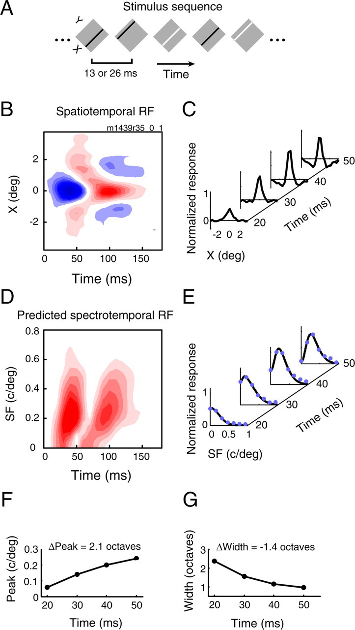
Prediction of SF tuning dynamics from spatiotemporal RFs. A, The stimulus sequence used to map spatiotemporal RFs was one-dimensional sparse noise. Elongated dark and light bars, aligned to a cell's preferred orientation, were randomly displayed at 20 or 30 positions over the RF. B, The spatiotemporal RF of an OFF-center cell. RFs are plotted as contour maps, where blue and red contours enclose dark and bright excitatory regions, respectively. For this and all other contour maps, each contour indicates a 10% decrement from the maximum amplitude. C, Time slices from 20 to 50 ms show the evolution of the spatial response over time, and in particular, the delayed development of the surround. D, Fourier analysis of the spatiotemporal RF yields the linear prediction of the spectrotemporal RF. E, Rightward tilted contours in the SF–time plane indicate coarse-to-fine dynamics, and time slices show a clear change from low to bandpass SF tuning. Solid blue dots mark data points whereas black curves show the DOG least-squares fit used to obtain tuning parameters for each time point. F, G, Graphs of tuning parameters over time. The peak SF (F) increases, and the half-width (G) decreases. Half- width is defined as follows: bw = log₂(SF_high/SF_peak), where SF_peak is the optimal SF and SF_high is the SF to the right of SF_peak at which amplitude falls to half the maximum value.

We used Fourier analysis to convert response functions from the spatial domain to the SF domain. For each time point of the spatiotemporal map, the spatial waveform is zero padded to fill a 1 × 32 vector. We then applied the fast Fourier transform to the data and analyze the resulting amplitude spectrum. This procedure assumes linear spatial summation of the RF, which is approximately true for the majority of LGN cells (Cai et al., 1997) (but see Bonin et al., 2005). This procedure is also highly dependent on the quality of the mapped RF. Because low signal in the spatial domain can bias responses toward lower frequencies, we limited our analysis to RFs, which are adequately mapped. This is determined objectively by setting a threshold for the signal-to-noise ratio (SNR) of the RF. The SNR is estimated as the SD of the spatial response at the peak correlation delay divided by the SD of the response occurring at negative time delays.

Subspace reverse correlation.

The procedures used for subspace reverse correlation are similar to those used in previous studies of SF dynamics (Bredfeldt and Ringach, 2002; Mazer et al., 2002; Nishimoto et al., 2005). Iso-oriented sinusoidal gratings at 50% contrast, with one of 15 SFs and eight spatial phases, are flashed for 26 ms in a randomized sequence over the RF of the cell. Blanks are not inserted in the stimulus sequence. Gratings are positioned and sized to completely cover the cell's RF, as determined with a preliminary coarse mapping procedure. Most gratings are between 3 and 6° in diameter. The appropriate range of logarithmically spaced SFs and the preferred orientation are determined beforehand with standard grating tests. Reverse correlation stimulus sequences are presented 150–300 times, after which they are cross-correlated with evoked responses to obtain a map of SF and spatial phase selectivity. Maps are calculated in 6 ms bins, the highest temporal resolution we can achieve while maintaining sufficient SNR for all cells. Because response maps are highly linear over phase, we combine phase information by taking the modulation across phases at each SF and correlation delay. This procedure captures all major features of the SF response maps. Three of 35 cells show slight suppression below baseline at very high frequencies over all phases. Although this feature is not captured in the modulating component, temporal dynamics of the tuning peak or width are not affected.

To compare direct measurements of SF temporal dynamics with predictions, we also map spatiotemporal RFs of the same cells with a two-dimensional (2D) dense noise version of reverse correlation (see Fig. 6A). In this paradigm, RFs are mapped with white noise stimuli generated according to binary m-sequences (for details, see Anzai et al., 1999). The stimulus grid, composed of 16 × 16 or 32 × 32 square elements, is updated with each display frame (13 ms). All other properties of the stimulus grid (position, width, and orientation) are identical to those in the subspace reverse correlation procedure, producing stimulus elements which are ∼0.25 × 0.25° in size. The resulting spatiotemporal RF has two spatial dimensions: Y, which is parallel to the preferred orientation of the cell, and X, which is orthogonal to Y. Because we measure SF tuning over the X dimension in our direct measurements (see Fig. 4A), we integrate the RF over Y before taking the Fourier transform and examining SF tuning.

Figure 6.

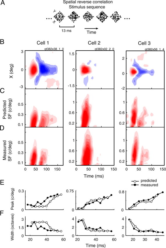
Predicted and measured SF tuning for three example cells. A, For comparing predicted and measured SF tuning, we used a slightly different version of spatial reverse correlation. Here, the stimulus sequence was 2D dense noise, where each frame displayed a 16 × 16 or 32 × 32 grid of black and white squares. B, Spatiotemporal RFs mapped with the sequence in A for three representative LGN cells. C, Predicted spectrotemporal RFs for each cell, obtained by taking the Fourier transform of their spatial maps. D, Measured spectrotemporal RFs, obtained with the stimulus depicted in Figure 3A. E, F, Temporal changes in the tuning peak (E) and half-width (F) are shown for both the predicted (open circles) and measured (filled circles) tuning curves.

Figure 4.

SF tuning dynamics measured with subspace reverse correlation. A, The stimulus for reverse correlation in the SF domain was a randomized sequence of iso-oriented sinusoidal gratings, each with one of 15 possible SFs and eight possible phases. Gratings were presented consecutively every two video frames (26 ms). B, Spectrotemporal RFs computed at each phase after 200 repetitions of the stimulus. Red and blue contours correspond to responses above and below the baseline level, respectively. C, Because responses are strongly linear with respect to phase, we compute the modulation over phase at each SF and correlation delay for further analysis. D, Time slices approximately spanning the first phase of the response reveal prominent changes in SF tuning. DOG fits (black curves) to the raw data (solid blue dots) were used to estimate tuning parameters. E, Both the peak SF (top) and the half-width (bottom) change over time in a coarse-to-fine manner.

We use dense noise rather than sparse noise to map the RFs for this analysis because it better matches the stimulus energy of the subspace reverse correlation sequence. Because stimulus energy can affect the latency, duration, and magnitude of responses, sequences should be comparable if meaningful comparisons are to be made (Albrecht, 1995). For both the sequence of sinusoidal gratings and the 2D m-sequence, stimuli cover the entire RF at all times, and the luminance across the grid always sums to the mean luminance (neither of which applies in the case of sparse noise).

SF tuning analysis.

SF tuning and dynamics are characterized identically for measured and predicted spectrotemporal RFs. In cases where multiple assessments of SF are made (see Fig. 7), analyses on each set of data are performed independently. For each spectrotemporal RF, we first determine the appropriate time points over which to perform a tuning analysis. The first time point (t_initial) is defined as the slice at which response variance exceeds that of the baseline by >5 SDs (Mazer et al., 2002). Baseline variance is calculated from noncausal delays. Determining the final time point at which to perform analysis is slightly more difficult because temporal response profiles of LGN cells are highly diverse. The majority of thalamic cells exhibit two response phases, although monophasic and triphasic profiles are also observed (Cai et al., 1997). In addition, the relative strengths between phases are heterogeneous: second (and third) phases are often a fraction of initial response, but many cells show additional phases of equal or (in a minority or cells) greater strength (Cai et al., 1997). For these reasons, we limit our analysis of SF tuning to the first phase of the response. The initial phase is also the most likely input to the “initial transient” response in cortical cells (Frazor et al., 2004; Nishimoto et al., 2005) and, therefore, is the most relevant response period to use when comparing geniculate SF tuning dynamics to those in visual cortex. Qualitatively, for cells with a strong biphasic response, the tilt of the second phase in the SF–time plane is similar to the tilt of the first phase. For many cells, second-phase response contours do not extend to SFs as high as during the first phase, although this could be caused by reduced SNR. A quantitative analysis comparing response dynamics between phases has not been performed. The end of the first phase, t_final, is defined as the time point at which response variance falls to a local minimum after the first peak. If no local minima are present, (i.e., monophasic response profiles), t_final is defined as the time point at which variance decreases to the baseline level. Using these criteria, the mean duration of the analysis window (t_initial to t_final) is 30.6 ms, with an SD of 7.9 ms.

Figure 7.

Population comparison of predicted and measured SF tuning. A, Scatter plot of predicted and measured high cutoff values for a sample of 28 neurons. There is a strong correlation (r = 0.97; p < 10⁻¹⁵, linear regression), although predictions clearly deviate from measurements. The differences between these values, computed as the log ratio of predicted SF_high to measured SF_high, are displayed in a histogram (top right). The mean difference is significantly different from zero (−0.22 ± 0.04 octaves, mean ± SEM; p < 10⁻⁵, two-tailed t test). B, Scatter plot of average predicted tuning peaks and measured tuning peaks. The data are highly correlated (r = 0.90; p < 10⁻⁹, linear regression) and most points lie above the y = x line, indicating a higher peak when SF tuning was measured directly. The mean difference, computed analogously to the difference in high cutoff, is significantly different from zero (−0.42 ± 0.16 octaves, mean ± SEM; p < 0.05, two-tailed t test). C, Scatter plot of the predicted changes and measured changes in tuning peak. The data are well correlated (r = 0.78; p < 10⁻⁶, linear regression) and points are roughly evenly distributed above and below the unity line. The differences between predicted and measured tuning changes are symmetrically distributed around zero. The mean of this distribution (3.6 × 10⁻⁴ ± 8.5 × 10⁻⁴ c/deg/ms, mean ± SEM) is not significantly different from zero (p > 0.5, two-tailed t test). D, A summary of SF tuning dynamics over the population of cells. Both predicted (dashed line) and measured (solid line) curves show a large shift from low-pass tuning at t_initial (left) to more bandpass tuning at t_final (right). However, for all time points, predicted tuning curves underestimate the true peak, as shown in B. Because this difference is roughly fixed over time, the predicted rate of peak change is relatively unaffected and correlates well to the measured value, as shown in C. Curves were generated by averaging the parameters of the best-fit DOG at the initial and final time point for each cell.

To characterize SF tuning dynamics, we examine the tuning peak and width at each time point in our analysis window. Before measuring these parameters, we fit the data with a difference of Gaussians (DOG) function to reduce susceptibility to noise. We find that the least-squares best fit (Levenberg–Marquardt algorithm) accounts for a large degree of the variance in the data (r² > 0.90 for 95% of curves). From the DOG fit, a cell's optimal SF at time t is defined as the SF at the peak of the tuning curve. Bandwidth is defined as log ratio of the high cutoff SF to the SF_peak:

where SF_high is the SF at which amplitude falls to half of the peak value. To estimate tuning changes over time, we compare parameters at initial and final time points. The change in peak is the log ratio:

and the change in bandwidth is the difference, Δbw = bw(t_final) − bw(t_initial).

Model structure.

To investigate the contribution of feedforward mechanisms to SF tuning dynamics in cortical cells, we model LGN–cortical connections with “push–pull” circuitry (Hubel and Wiesel, 1962; Jones and Palmer, 1987; Ferster, 1988; Reid and Alonso, 1995; Hirsch et al., 1998; Troyer et al., 1998). Other push-only models such as the structural model described in Frazor et al. (2004) could have been used, but this construction does not account for the sharpening in the low-frequency limb of the SF tuning curve, nor is it consistent with pharmacological experiments showing this sharpening involves inhibitory circuitry (Bauman and Bonds, 1991; Vidyasagar and Mueller, 1994; Pernberg et al., 1998). Our model accounts for general aspects of cortical SF tuning, although its scope is limited. We consider only responses of layer IV simple cells, receiving excitatory input from nonlagged LGN cells with central RFs and biphasic temporal structure. Simple cells are modeled as having two dominant RF subregions that do not vary systematically in position over time (i.e., nondirection selective). In addition, our model does not include known structural and biophysical mechanisms, such as expansive output nonlinearities, spike thresholds, or intracortical correlation-based excitation. We exclude these factors to reduce the number of free parameters and to keep the model as simple and interpretable as possible. Previous work (Troyer et al., 1998) has demonstrated that full incorporation of these mechanisms in a computational model produces similar behavior to a more conceptual version. This suggests that a more complex construction might alter the exact numerical results in our simulations, but would not change the general outcome.

For each simulation, we construct one excitatory and one inhibitory cortical cell whose RFs are 180° out of phase. LGN inputs are combined to form cortical cells using rules of connectivity between thalamic and cortical simple cells (Alonso et al., 2001). For simplicity, cortical RFs are modeled as having two primary subregions, although weaker flanking subregions are also present because of LGN RF structure (see Fig. 9, cortical RFs). Primary subregions are separated by 1°, the average distance between subregions from our own database of cortical RFs (data not shown). Each subregion receives input from 15 LGN cells whose positions are drawn from a normal distribution with mean equal to the center of the subregion and an SD of 0.15° (Alonso et al., 2001). The sizes of LGN RF centers are distributed around the widths of the subregions (Alonso et al., 2001), described in greater detail below. In preliminary simulations, we covaried input efficacy with the overlap of geniculate and cortical RFs and also used a “same sign” rule with a probability of 70% in accordance with Reid and Alonso (1995) (Alonso et al., 2001). However, the small number of LGN inputs led to highly variable cortical RFs with occasional atypical organization. Therefore, in the final version of the model, all LGN cells contributing to a single subregion share the same sign and have equal efficacy. Intracortical connections between cells with similar RF structure, which are not included in this model, could function to increase stability and robustness of cortical cells, as has been proposed previously (Troyer et al., 1998).

Figure 9.

Effect of different model parameters on cortical tuning dynamics. A–C, Each diagram (top) illustrates the model parameter being explored and the effect on the cortical RF. Parameter values increase from left to right. Graphs (bottom) show the mean ± SEM shift in peak SF as a function of the model parameter, obtained after 15 simulations. Each set of simulations focused on a single variable; the other two parameters were fixed at zero and the inhibitory weight (W) was set to 1.25. Blue circles indicate average values found in previous studies (Ferster, 1988; Cai et al., 1997; Hirsch et al., 1998; Weng et al., 2005), which are also used in inhibitory weight simulations (Fig. 8). A, Cortical shift in peak SF as a function of the time delay between the center and surround in LGN RFs. B, Cortical shift in peak SF as a function of the slope relating response latency to RF size. A negative slope indicates that cells with larger RFs have shorter latencies than cells with smaller RFs. C, Cortical shift in peak SF as a function of the time delay (τ) between the arrival of excitation and inhibition in a cortical cell.

LGN RF parameters.

Spatiotemporal LGN RFs are modeled as in Cai et al. (1997). Spatial profiles are described with a DOG, and temporal profiles are described as a difference of gamma functions, with distinct center and surround components. The full expression is RF(x,t) = F_c(x)G_c(t) − F_s(x)G_s(t), where

and F_s(x) is defined analogously. The temporal filter for the center is as follows:

Most parameters are fixed to the geometric means of their distributions as reported in Cai et al. (1997): A_s/A_c = 0.3; K₁ = 1.05; c₁ = 0.14; n₁ = 7; K₂ = 0.7; c₂ = 0.12; n₂ = 8. During simulations which do not include space–time correlations (see Fig. 9A,C), t₁ and t₂ are held constant at −6 ms. This set of parameters produces a biphasic temporal profile with a fast, initial phase which peaks at 38 ms and a slower, weaker second phase which peaks at 85 ms and decays fully by 150 ms. Because it is unlikely that all geniculate inputs which converge onto a single simple cell have identical temporal profiles (Alonso et al., 2001), we performed additional simulations in which response latency was permitted to vary. As expected, this addition increases the variability in cortical output, but otherwise yields results identical to those produced with a fixed t₁ and t₂.

The distribution of LGN RF sizes contributing to a single cortical cell is based on previous reports (Alonso et al., 2001). These data show that LGN RF centers are typically equal to or slightly greater than the subregion width of the cortical cell, although geniculate cells with RF centers larger than two times the subregion width also contribute input, although with reduced frequency. To approximate this distribution for a subregion separation of 1°, the RF center diameter is drawn from N_(0.8,0.36) ≥ 0.7° (i.e., a modified Gaussian distribution with mean 0.8° and SD 0.6°, rectified <0.7°). The median of this distribution is 1.15°, and ∼15% of inputs have a RF center that is more than two times the cortical subregion width.

From the LGN RF center, we derive the size of the RF surround and the temporal response function. The size of the surround is related to the size of the center by σ_s = 1.5 × σ_c + 0.4, a linear relationship found in previous model fits of LGN spatiotemporal RFs (Cai et al., 1997) (r² = 0.41; p < 10⁻⁶, linear regression). To incorporate correlations between thalamic RF size and response latency (Weng et al., 2005), we can delay or advance the temporal profile by adjusting parameters t₁ and t₂. Note that changing t₁ and t₂ corresponds to a simple shift along the time axis, not a stretching or contracting of the curve. For each cell, the time shift is computed by first finding the difference in RF center area (assuming circularly symmetric RFs):

where d_c is the center diameter of each LGN cell, and d_m is the median center diameter from the distribution, 1.15°. We multiply the difference in area, D, by a space–time slope [in milliseconds per degree squared (ms/deg²)] to obtain the temporal shift, which is added to t₁ and t₂. Space–time slopes are all negative, such that cells with larger RF centers have shorter latencies. For reference, a space–time slope of −3.5 ms/deg² produces a population of LGN RFs with optimal latencies separated by ∼10 ms. This separation is similar to the measured difference in peak latencies between connected geniculate and simple cells, ∼5–15 ms (Alonso et al., 2001).

Model simulations.

To measure the SF tuning of our model cortical cells, we calculate LGN responses to static sinusoidal gratings at different SFs, ranging from 0.01 to 1.5 cycles (c)/deg, and four different phases. Thalamic input to cortical cells is calculated as the sum of the rectified firing rates of each LGN cell, with a geniculate spontaneous firing rate of 10 spikes/s. In addition to excitatory thalamic input, the cortical cell receives input from the inhibitory cortical cell, which is antiphase inhibition parameterized by a weight, W, and a time delay, τ. The total input to the excitatory cortical cell can be expressed as follows:

where

is the combined output from all the LGN cells connecting to a cortical cell in response to a sinusoidal grating, S, at SF, f, and phase φ. LGN_e represents the response from cells connecting directly to the excitatory cell (see Fig. 8A), whereas LGN_i refers to responses from cells connected to the inhibitory cell (see Fig. 8B). For simplicity, we have treated the inhibitory response as linear: the effective inhibitory current in the excitatory cell is simply a weighted version of the output from LGN cells (LGN_i), with an additional temporal shift to account for the disynaptic pathway. To obtain output from the excitatory cell, the input is integrated with a time constant of 10 ms and rectified.

Figure 8.

A feedforward model examining mechanisms of SF dynamics in cortex. A, B, Responses of simple cells are modeled with a push–pull circuit. Excitatory input (A) to a cortical cell comes from spatially offset, although still overlapping, ON- and OFF-center LGN cells. The offset is exaggerated in this illustration for clarity. Inhibition (B) is provided by LGN cells with identical spatial position but opposite phase, after being routed through a cortical interneuron. The inhibition is parameterized with a time delay (τ) between excitation and inhibition, and a weight (W), which gives the relative level of inhibition compared with excitation.

Following protocols used in previous studies of cortical SF dynamics (Bredfeldt and Ringach, 2002; Frazor et al., 2004; Nishimoto et al., 2005), full spectrotemporal maps for each cortical cell are obtained by averaging responses to stimulus gratings across all phases. Tuning shifts are then calculated by comparing parameters from time points at which response variance rises or falls to 20% of the maximum value. The duration of this time period is ∼40 ms, facilitating comparisons to earlier reports (Frazor et al., 2004; Nishimoto et al., 2005). Because our model permits the precise position and size of LGN RFs to vary, we repeat simulations with each set of parameters 15 times.

Results

Our results are organized into three sections. First, we describe the SF dynamics observed in a large population of LGN cells as predicted from spatiotemporal RFs. Second, we assess the validity of these predictions using a subspace reverse correlation technique for a sample of cells. Third, we present a simple model, based on push–pull circuitry, which examines the extent to which cortical tuning changes can be explained by feedforward input.

Predicted SF dynamics

We analyzed responses of 118 LGN cells from our electrophysiology database for which the spatiotemporal RF of each unit was mapped using one-dimensional sparse noise reverse correlation (Fig. 1A). The spatiotemporal RF for a typical LGN neuron in our sample is shown in Figure 1B. RFs are plotted as contour maps, which indicate dark (blue) and bright (red) excitatory regions. A feature evident in the RF of this OFF-center cell is the delay of the surround response with respect to the center, a property common to most LGN neurons (Cai et al., 1997). Slices through different time points in the RF (Fig. 1C) show the temporal evolution of the spatial profile more clearly. At t = 20 ms, the center response is already present, but the surround response does not fully develop until t = 40 ms.

This characteristic temporal inseparability in the spatial domain predicts corresponding changes in the spectral domain. The spectrotemporal RF, obtained by taking the Fourier transform of the spatiotemporal RF, is shown in Figure 1D. This cell is strongly biphasic, and exhibits two distinct response regions, both of which are slightly slanted in the SF–time plane. This slanting indicates dynamic SF tuning. Time slices through the spectrotemporal RF (Fig. 1E) show that SF tuning is low-pass and broad at time points during which only the center is present (Fig. 1C). The later development of the surround suppresses responses to very low SFs, and the tuning becomes bandpass.

To quantify tuning changes, we find the optimal SF (Fig. 1F) and tuning width (Fig. 1G) for each time point, and then calculate the changes in these values over time. We fit the data (Fig. 1E, blue dots) with a DOG function (Fig. 1E, black lines) to improve our estimation of tuning parameters. For cells with multiphasic temporal profiles, we limit our analysis to points spanning only the first phase of the response (∼30 ms), because some cells have a substantially weaker second phase which may not be captured well by the RF mapping procedure.

The distributions of average tuning parameters (Fig. 2A,B) and the temporal shifts in these parameters (Fig. 2C,D) are shown for our sample of LGN cells. Average tuning curves are obtained by integrating the spectrotemporal response from t_initial to t_final, where t_initial is the first time point used in our analysis [e.g., t = 20 (Fig. 1)], and t_final is the last. The distribution of optimal SF (Fig. 2A) is broad, ranging from 0.01 to 0.75 c/deg, with a mean of 0.26 c/deg. Figure 2B summarizes the tuning bandwidths found in this population. The low selectivity exhibited by most LGN cells (Lehmkuhle et al., 1980; Troy, 1983) is evident, as most half widths are >0.8 octaves. For comparison, cells in the primary visual cortex typically have tuning half-widths between 0.3 and 0.8 octaves (Movshon et al., 1978; Nishimoto et al., 2005).

Figure 2.

Population distributions of predicted tuning parameters and parameter changes over time. A, B, Histograms of the peak SF (A) and half-width (B) for our sample of LGN neurons (n = 118). Average tuning parameters describe the tuning curve obtained by integrating the spectrotemporal map from t_initial to t_final (∼30 ms). C, D, Distributions of changes in peak SF and tuning width. Peak shift is defined as log₂[SF_peak(t_final)/SF_peak(t_initial)], and the shift in width is bw(t_final) − bw(t_initial). Both the mean of the peak shift (1.14 ± 0.076 octaves, mean ± SEM) and the mean of the width shift (−0.95 ± 0.072 octaves, mean ± SEM) were significantly different from zero (p ≈ 0 and p ≈ 0, two-tailed t test).

We now examine SF tuning as a function of response latency. If SF tuning is temporally static, the parameters describing tuning curves at each time point will be similar, and the shifts in these parameters should be distributed evenly around zero. However, for our LGN sample, shifts in tuning peak (Fig. 2C) are distributed almost entirely above zero (i.e., preferred SF changes from low to high values during the course of the cell's response). On average, the optimal SF changes by over an octave (1.14 ± 0.076 octaves, mean ± SEM). Similarly, the shifts in tuning bandwidth (Fig. 2D) are nearly all distributed over negative values, corresponding to a narrowing of the curve, or a selectivity increase with greater latency. The mean of this distribution is −0.95 ± 0.072 octaves.

Direct measurements of SF dynamics

Accurate predictions of SF tuning from spatiotemporal RFs require that (1) the spatiotemporal RF of the cell is completely captured with the mapping procedure, and (2) the cell's response is linear. Requirement 1 is highly dependent on the properties of the stimulus used to map the RF. In the spatial domain, large stimuli will blur fine features, biasing results toward lower SFs. Small stimuli, however, may not excite the cell sufficiently to reach threshold. These effects are illustrated in Figure 3, which shows the spatiotemporal and spectrotemporal RFs of a single cell mapped with two different stimulus grid sizes. The RFs achieved with large (Fig. 3A,C) and small (Fig. 3B,D) stimulus grids are similar, but substantial differences are immediately obvious. The spatiotemporal RF obtained with large stimuli (Fig. 3A) exhibits a strong surround in both phases of the response. In comparison, the surround response of the RF mapped with smaller stimuli (Fig. 3B) is considerably weaker in the first phase, and almost nonexistent in the second. As a consequence, the SF response of the second phase (Fig. 3D) is predominately low-pass and shows little of the dynamics clear in the spectrotemporal map obtained with large stimuli (Fig. 3C). However, the large pixels are incapable of capturing the full narrowing of the center component over time. Compared with the fine stimuli spectrotemporal map (Fig. 3D), this leads to a noticeable decrease in the high SF cutoff (Fig. 3C).

Figure 3.

Spatiotemporal RFs of a single neuron obtained with different stimulus grid sizes. A, C, The mapped spatiotemporal RF (A) and predicted spectrotemporal RF (C) obtained with an 8 × 8 stimulus grid. B, D, The mapped spatiotemporal RF (B) and predicted spectrotemporal RF (D) obtained with a 16 × 16 stimulus grid. Black boxes along the X dimension of the spatiotemporal RFs show the positions and sizes of each stimulus pixel. The stimuli used in A are too large to capture the full narrowing of the center component which is seen in B. This corresponds to a reduction in the high SF cutoff in the SF domain (compare C, D). However, the large stimuli are much more effective in eliciting a response from the surround.

Requirement 2, LGN cell response linearity, has been addressed previously (Derrington and Lennie, 1984; Dan et al., 1996; Cai et al., 1997). We note that nonlinear phenomena are present in LGN responses, and that the nonlinear component can be modeled with a suppressive field, preferentially tuned to low SFs (Bonin et al., 2005). Although studies suggest that nonlinear contributions to LGN responses are small, SF-specific suppression with a distinct time course might have large effects on the temporal evolution of the response, and therefore must be considered in this study. To provide a more definitive analysis of LGN SF dynamics, we have measured SF tuning directly as a function of time.

These measurements are conducted using a subspace reverse correlation procedure (Bredfeldt and Ringach, 2002; Mazer et al., 2002; Nishimoto et al., 2005) (Fig. 4A). A randomized sequence of sinusoidal gratings, flashed briefly over the cell's RF, is cross-correlated with the evoked spike train to obtain a 2D map of SF and spatial phase selectivity (Fig. 4B). For the cell shown in Figure 4 and all others (n = 35), the response is sinusoidal as a function of phase. Stimuli evoking responses at one phase (e.g., red contours at 0°) reduce those at the antiphase below baseline level (e.g., blue contours at 180°). This response property enables us to construct a single spectrotemporal RF for each cell by calculating the modulation amplitude across phase for each SF and correlation delay (Fig. 4C). Note that this procedure is analogous to taking the F1 component of a response to a drifting grating. From the modulation spectrotemporal RF, tuning dynamics are assessed using the same procedure that is applied to the predicted spectrotemporal RFs from the database.

Tuning for the example cell is clearly dynamic. Response contours in the SF–time plane tilt slightly to the right (Fig. 4C), and slices at different time points show a gradual shift from low-pass to bandpass tuning (Fig. 4D). The preferred SF (Fig. 4E, top) shifts to higher values over time, and bandwidth narrows (Fig, 4E, bottom). These tuning properties are representative of those observed for our sample of cells, shown in Figure 5. Thirty-two of 35 neurons show a change in optimal SF from low to high values, with an average shift of 1.8 ± 0.2 octaves (mean ± SEM) (Fig. 5C). Likewise, tuning selectivity increases with correlation delay for 31 of 35 cells (Fig. 5D). On average, bandwidth narrows by −0.84 ± 0.17 octaves. From these data, we conclude that SF tuning follows a coarse-to-fine processing sequence for nearly all LGN neurons.

Figure 5.

Population distributions of measured tuning parameters and parameter changes over time. A, B, Histograms of the peak SF (A) and half-width (B) obtained with subspace reverse correlation for a sample of 35 LGN neurons. C, D, The distributions of changes in peak SF and tuning width. Both the mean of the peak shift (1.8 ± 0.20 octaves, mean ± SEM) and the mean of the width shift (−0.84 ± 0.17 octaves, mean ± SEM) are significantly different from zero (p < 10⁻⁹ and p < 0.0001, respectively, two-tailed t test).

For 28 of the 35 neurons, we also mapped the spatiotemporal RF to compare predicted and measured spectrotemporal tuning. Because stimulus energy affects temporal response characteristics (Albrecht, 1995), we used a 2D dense noise sequence (Fig. 6A) to better match the energy of the stimulus used for subspace reverse correlation (Fig. 4A). Results for three example cells are shown in Figure 6. Data for each neuron are organized into columns, with rows showing the spatiotemporal RF (Fig. 6B), the predicted spectrotemporal RF obtained from Fourier analysis (Fig. 6C), the measured spectrotemporal RF (Fig. 6D), the peak SF over time (Fig. 6E), and the tuning width over time (Fig. 6F).

A qualitative comparison of measured and predicted spectrotemporal tuning suggests that gross response characteristics are well matched. The SF ranges over which each cell responds and the temporal profiles (i.e., strongly biphasic for cell 1, monophasic for cell 2) correspond well. In addition, the parameters describing measured and predicted tuning show similar changes over time (Fig. 6E,F). However, a systematic deviation in tuning is also evident: for all three neurons, the high SF cutoff is higher in the measured case (Fig. 6, compare C, D).

A more quantitative comparison of high SF cutoffs between measured and predicted tuning is presented in Figure 7A. A scatter plot of the data reveals a strong correlation (r = 0.97), although predictions consistently underestimate measured values, particularly at higher SFs. Differences between predicted and measured high cutoffs (projected in the histogram orthogonal to the unity line) are all less than zero, with a mean difference of −0.22 ± 0.04 octaves.

A similar relationship exists between the predicted and measured average optimal SF (Fig. 7B), although differences are less pronounced. Predicted and measured peaks are well correlated (r = 0.90), but most points lie above the unity line, indicating that predictions underestimate true values. Correspondingly, the distribution of differences in the peak (Fig. 5B, top right) is skewed toward negative values, with a mean of −0.42 ± 0.16 octaves.

Predicted and measured rates of change in SF_peak are plotted in Figure 7C. Rates of change are more appropriate for comparisons than absolute shifts because analysis time points are determined independently for the different data sets and durations can differ by as much as 15 ms. The rate of change of preferred SF (in cycles per degree per millisecond) is the slope of the best fit line to the time versus the SF_peak curve (Fig. 6E). The scatter plot in Figure 7C shows that measured and predicted tuning changes are correlated (r = 0.78), and that there are no systematic deviations in the predictions. Points lie about evenly above and below the y = x line, and the distribution of differences is centered close to zero (3.6 × 10⁻⁴ ± 8.5 × 10⁻⁴ c/deg/ms).

These data are summarized in Figure 7D, which provides comparisons of predicted and measured tuning curves, averaged over all cells, for t_initial (left) and t_final (right). Predicted tuning curves (dotted lines) peak at lower SFs than measured curves (solid lines) and underestimate responses to higher SFs. These deviations could result from nonlinear contributions or from biases in the mapping procedure (see Discussion). However, because the differences in tuning are somewhat consistent over time, predicted tuning changes are close to the measured values. From this, we conclude that linear predictions of spectrotemporal RFs provide good estimates of SF tuning dynamics for LGN neurons.

Relating coarse-to-fine dynamics in LGN and visual cortex

Previous studies have demonstrated coarse-to-fine SF tuning in the visual cortex (Bredfeldt and Ringach, 2002; Mazer et al., 2002; Frazor et al., 2004; Nishimoto et al., 2005). Our current results raise an obvious question: how much of the cortical effect can be accounted for by feedforward processing from early visual pathways? To address this, we used a model relating thalamic input to the first stage of cortical output (see Materials and Methods for full model details).

Our model uses push–pull circuitry, based on numerous studies of extracellular and intracellular recordings from LGN and the primary visual cortex (Hubel and Wiesel, 1962; Jones and Palmer, 1987; Ferster, 1988; Reid and Alonso, 1995; Hirsch et al., 1998). It is similar in structure to a model developed previously to explore contrast invariant orientation tuning (Troyer et al., 1998). A schematic of the model is presented in Figure 8. Spatially offset ON and OFF LGN cells (represented by their RFs in Fig. 8A) provide excitatory input (push) to distinct ON and OFF subregions of a cortical cell. LGN cells with identical spatial configuration and opposite phase (Fig. 8B) provide inhibitory input (pull) to the cortical cell, after routing through a cortical inhibitory interneuron. Inhibition is parameterized with a weight, W, relative to the level of excitation, and a time, τ, which describes the delay of inhibition relative to excitation.

As described previously (Ferster, 1988; Troyer et al., 1998; Lauritzen and Miller, 2003), this arrangement of inputs can filter spatial information. When inhibition has an equal to or greater weight than excitation (W ≥ 1), only stimuli that preferentially excite one phase of LGN cells (Fig. 8A,B) pass through the filter to produce a response in the excitatory cortical cell. These properties are instrumental in constructing cortical SF tuning. Stimuli at very low SFs excite neighboring ON and OFF LGN cells equally. Thus, downstream cortical neurons are simultaneously excited and inhibited and fail to fire. In contrast, stimuli at higher SFs excite the phases of LGN cells differently to produce a robust response in the excitatory cortical cell. The push–pull configuration thus sculpts the typically low-pass SF tuning of thalamic input into the more bandpass tuning characteristic of cortical neurons.

Within the structure of the push–pull model, we examine several sources of dynamic input which could lead to SF changes in layer IV simple cells. These include (1) mechanisms within single cells (the time delay between center and surround responses in LGN RFs), (2) mechanisms across a population of cells (the correlation between response latency and RF size reported previously) (Derrington and Fuchs, 1979; So and Shapley, 1979; Sestokas and Lehmkuhle, 1986; Weng et al., 2005), and (3) mechanisms within a network (the time delay between feedforward excitation and feedforward inhibition). For each of these mechanisms, we incrementally vary model parameters and measure SF tuning of the model cortical cells.

Shifts in cortical SF tuning originating from different types of spatiotemporal dynamics are depicted in Figure 9. Increasing the time delay (td) between the LGN RF center and surround produces noticeable changes in the geniculate and cortical RFs (Fig. 9A, top). The simple cell has two primary subregions (i.e., LGN centers “map” to two regions), although flanking subregions also develop because of the LGN surround responses. The timing of the weaker flanking subregions is directly affected by the LGN center-surround delay, and these subregions lag behind the dominant subregions for td > 0. This aspect of the model simple cell RF is in agreement with experimental results showing that the weakest cortical RF subregions have the slowest time courses (Alonso et al., 2001).

As the slower flanking subregions develop they narrow the primary subregions, shifting the SF tuning curve to higher frequencies (Fig. 9A, bottom). Changing td from 0 to 12 ms, the shift in tuning peak rises significantly from 0 to 0.5 octaves (p ≈ 0, one-way ANOVA). Varying the center-surround delay also affects the average SF tuning peak, although only optimal SFs from td = 0 ms (0.43 ± 0.006 c/deg) and td = 12 ms (0.41 ± 0.006 c/deg) are significantly different (p < 0.05, one-way ANOVA with Tukey's honest significant difference criterion). The average time delay observed in LGN neurons, ∼6 ms (Fig. 9A, blue circle) (Enroth-Cugell et al., 1983; Cai et al., 1997) produces a cortical SF tuning shift of 0.35 octaves. This value is consistent with measurements of SF shifts for simple cells in the visual cortex, which range from 0.2 to 0.6 octaves and average to ∼0.5 octaves (Bredfeldt and Ringach, 2002; Frazor et al., 2004; Nishimoto et al., 2005).

A second source of spatiotemporal dynamics is the correlation between RF size and response latency (Fig. 9B, top). For cells responding to overlapping regions of visual space, this relationship is strongly linear (Weng et al., 2005) and can be parameterized as a negative slope in the space–time plane with units of ms/deg². Implementing this space–time slope into the model produces a gradual narrowing of cortical RF subunits over time because LGN cells with smaller RFs respond at longer latencies. As the space–time slope increases in amplitude, the time between responses from large and small LGN cells grows, and the shift in cortical SF tuning peak increases significantly (Fig. 9B, bottom) (p < 10⁻¹⁴). Changes in preferred SF as a result of space–time correlations are of a similar magnitude as those found with the center-surround time delay, reaching ∼0.3 octaves at a slope of −7 ms/deg². As expected, increasing the slope affects the duration of the cortical response, but does not alter the average tuning peak (mean ± SEM ranges from 0.43 ± 0.006 c/deg at slope = 0 to 0.42 ± 0.006 c/deg at slope = −7 ms/deg²; p > 0.5). A typical slope relating size and latency, estimated as −3.5 ms/deg² in a study by Weng et al. (2005), produces a cortical SF tuning shift of ∼0.15 octaves.

The final type of temporally dynamic input examined here is the time delay (τ) between excitatory and inhibitory input (Fig. 9C, top). Because the pathway for feedforward inhibition requires two synapses (thalamocortical and corticocortical), the onset of inhibition is delayed with respect to excitation. Intracellular recordings from layer IV simple cells in the primary visual cortex show this delay to be ∼5 ms (Ferster, 1988; Hirsch et al., 1998) (Fig. 9C, bottom, blue circle). Our simulations indicate that the inhibitory delay generates a significant coarse-to-fine SF shift in cortical tuning (p < 10⁻¹¹), although the magnitude of this effect is quite small compared with other sources of dynamic input. At τ = 10 ms, the inhibitory time delay produces a shift of only 0.06 ± 0.005 octaves, suggesting that it is not the primary mechanism underlying SF tuning dynamics in the visual cortex.

In the previous simulations, the weight of inhibition (W) is fixed at a value of 1.25 (i.e., it slightly exceeds the level of excitation). This value of W is used because it produces SF tuning curves with realistic bandwidths (0.6–0.7 octaves), and is consistent with experimental (Hirsch et al., 1998) and theoretical (Troyer et al., 1998) studies demonstrating the presence and possible function of slightly dominant inhibition. However, because inhibition plays a critical role in shaping cortical tuning, we must also examine how the level of inhibition affects tuning dynamics. In the following simulations, we parametrically vary W while holding other variables fixed at the average values marked with blue circles in Figure 9.

Results from these simulations show that increasing the weight of feedforward inhibition (Fig. 10A) produces dramatic changes in the average SF tuning peak (Fig. 10B) and the shift in tuning peak over time (Fig. 10C). As W increases from 0 to 2, the optimal SF changes significantly from ∼0.32 to 0.42 c/deg, and the peak shift decreases from ∼1 to 0.4 octaves (p ≈ 0 for both). Full spectrotemporal RFs from sample model cells (Fig. 10D) provide an explanation of these effects. When inhibition is absent (W = 0, left), SF dynamics are similar to those observed in LGN cells (compare with Figs. 6D, 10D). The strongly low-pass response at short latencies leads to a large shift in optimal SF (>1 octave), which is comparable with changes observed in the LGN, but is considerably higher than average values observed in simple cortical cells (Bredfeldt and Ringach, 2002; Frazor et al., 2004; Nishimoto et al., 2005).

Figure 10.

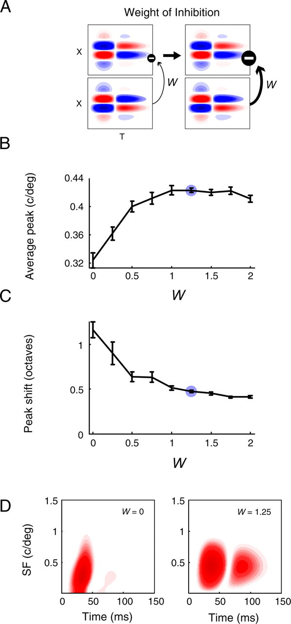
Effect of inhibitory weight on cortical tuning dynamics. A–D, For simulations in which we vary the weight of inhibition (W), all other parameters are held fixed at the values marked by blue circles in Figure 9 (LGN center-surround delay, 6 ms; size-latency slope, −3.5 ms/deg²; inhibitory delay, 5 ms). The blue circles in B and C of this figure indicate the value of W used for simulations in Figure 9. A, A diagram depicting an increase (from left to right) in the weight of feedforward inhibition. B, The average peak SF increases as a function of W. C, The shift in peak SF decreases as inhibition increases, and plateaus at 0.4 octaves. D, Spectrotemporal RFs from the model elucidate the trends in B and C. Without inhibition (W = 0, left), cortical SF tuning mimics that of the LGN (compare with Fig. 4D): the initial response is low-pass, and over time the peak SF changes more than an octave. With relatively strong inhibition (W = 1.25, right), only stimuli that preferentially excite LGN cells of a single phase (i.e., stimuli with higher SFs) will produce a response in the cortical cell. Thus, the initial response is bandpass, and more moderate peak changes (∼0.4 octaves) occur as a result of input dynamics.

When the level of inhibition is increased (W = 1.25) (Fig. 10D, right), spectrotemporal dynamics are markedly different. SF tuning is initially bandpass and exhibits a moderate refinement and shift to higher frequencies with greater latencies. We find that for inhibition equal to or greater than the level of excitation, the average preferred SF (∼0.42 c/deg) and shift in tuning peak (∼0.45 octaves) of our modeled cortical cells are in good agreement with experimental results (Movshon et al., 1978; Bredfeldt and Ringach, 2002; Frazor et al., 2004; Nishimoto et al., 2005). This suggests that feedforward dynamic input can account for the SF tuning changes observed in the primary visual cortex, and that additional refinement from intracortical circuitry may not be necessary.

Discussion

Our experiments in the LGN demonstrate that coarse-to-fine processing of spatial features originates in precortical structures. This effect can be largely accounted for by the temporal delay between center and surround components of the RF, although significant differences exist between measurements and linear predictions of SF tuning dynamics. In general, measured values of peak and high cutoff SFs are higher than their predictions. There are several potential factors that may account for this. First, the sampling grid of the spatial reverse correlation stimuli may bias the SF tuning toward lower values. If the sampling grid is not fine enough, the RF mapping procedure cannot resolve potential size changes of center/surround components. Smaller stimulus impulses can combat this problem, although they may not provide enough energy to elicit spike discharge. This is particularly true for the weaker surround (Fig. 3), which may be consistently underrepresented. A second factor that may explain this discrepancy is the contribution of SF-specific input that is activated differently by the oriented stimuli in the subspace reverse correlation procedure versus the individual pixels in spatial reverse correlation. A likely source of nonlinear input is the perigeniculate nucleus, which responds preferentially to large, low-frequency stimuli and provides inhibitory feedback to relay cells in the LGN (So and Shapley, 1981; Price and Morgan, 1987; Xue et al., 1988; Funke and Eysel, 1998).

Despite the differences between measured and predicted SF tuning, the rates of tuning changes are closely matched (Fig. 7D). This suggests that the SF tuning dynamics are largely a consequence of the spatiotemporal inseparabilities in the LGN RF structure. The center/surround temporal organization of LGN neurons is inherited from retinal ganglion cells, although LGN surrounds are typically more pronounced than those of their retinal inputs (Bullier and Norton, 1979; Usrey et al., 1999; Ruksenas et al., 2000). Thus, it is probable that coarse-to-fine processing begins at the first stage of the visual system, and is then enhanced in the thalamus.

To examine how dynamic thalamic input might affect SF tuning in the visual cortex, we incorporated spatiotemporal inseparabilities into a feedforward model. We find that both the center-surround delay in LGN RFs and the correlation between RF size and response latency are capable of producing cortical SF tuning changes similar in magnitude to those found experimentally (Bredfeldt and Ringach, 2002; Frazor et al., 2004; Nishimoto et al., 2005). Although our current study is the first to identify feedforward dynamics within LGN cells as a mechanism underlying cortical SF tuning dynamics, the space–time relationship observed across a population of cells has been proposed previously (Mazer et al., 2002; Frazor et al., 2004). Using a structural model, Frazor et al. (2004) found that the different response characteristics of magnocellular and parvocellular cells in primate LGN could account for a large portion of tuning dynamics measured in the visual cortex.

Convergence of magnocellular and parvocellular inputs, or X and Y inputs in the cat (So and Shapley, 1979; Sestokas and Lehmkuhle, 1986), can produce shifts in preferred SF as a function of response latency. However, it cannot explain the SF-specific suppression that was reported by Bredfeldt and Ringach (2002). In this study of cortical SF dynamics, we found a delayed “suppressive component” that was typically centered at low SFs. This finding is supported by several previous reports demonstrating inhibitory refinement of cortical SF tuning, particularly at the low-frequency limb of the curve (Bauman and Bonds, 1991; Vidyasagar and Mueller, 1994; Pernberg et al., 1998). Suppression at low SFs has been previously attributed to an intracortical network (Bredfeldt and Ringach, 2002). However, we find that this suppression emerges as a property of the push-pull configuration (i.e., feedforward inhibition) and, thus, it is not necessary to invoke additional cortical circuitry.

It is interesting to note that the dynamic push–pull model that we use has general applications and makes additional predictions of temporal responses in the cortex. In the simulations presented here, we consider only inputs to simple cells. However, there is evidence that some layer IV complex cells achieve phase invariance by receiving “push” from both phases of LGN cells (Hirsch et al., 2003). In these complex cells, SF tuning would be broader and more low-pass than tuning in simple cells, a difference that is reported in several studies (Movshon et al., 1978; Bauman and Bonds, 1991; Vidyasagar and Mueller, 1994). Because these cells might receive primarily antiphase excitation (as opposed to inhibition), they would undergo large SF tuning shifts over time, similar to the W = 0 case in Figure 10D. Notably, observed tuning shifts are approximately twice as large in complex cells (∼1 octave) as in simple cells (∼0.5 octaves) for both the cat and primate visual cortex (Frazor et al., 2004).

In conclusion, our results support coarse-to-fine spatial processing as a general property of information transmission in the visual system, and help to clarify the physiological processes underlying sequential analysis. Dynamic spatial processing begins early in the visual pathway, presumably within the retina (Enroth-Cugell et al., 1983), and propagates via several mechanisms to higher visual areas with more specialized functions (Ringach et al., 1997; Pack and Born, 2001; Bredfeldt and Ringach, 2002; Mazer et al., 2002; Menz and Freeman, 2003; Frazor et al., 2004; Nishimoto et al., 2005). Furthermore, recent work suggests that coarse-to-fine processing is not limited to visual processing. Spatiotemporal RFs of cells in peripheral and central structures of the somatosensory pathway exhibit inseparabilities that generate refined representation of tactile information with increased latency (Sripati et al., 2006). In addition, models of spectrotemporal RFs in the auditory cortex show that discrimination of complex stimuli is enhanced by delayed inhibition in a push–pull circuit (Narayan et al., 2005). Considered together, these studies point to coarse-to-fine processing as a fundamental coding strategy in the CNS.

References

- Albrecht DG. Visual cortex neurons in monkey and cat: effect of contrast on the spatial and temporal phase transfer functions. Vis Neurosci. 1995;12:1191–1210. doi: 10.1017/s0952523800006817. [DOI] [PubMed] [Google Scholar]
- Alonso JM, Usrey WM, Reid RC. Rules of connectivity between geniculate cells and simple cells in cat primary visual cortex. J Neurosci. 2001;21:4002–4015. doi: 10.1523/JNEUROSCI.21-11-04002.2001. [DOI] [PMC free article] [PubMed] [Google Scholar]
- Anzai A, Ohzawa I, Freeman RD. Neural mechanisms for encoding binocular disparity: receptive field position versus phase. J Neurophysiol. 1999;82:874–890. doi: 10.1152/jn.1999.82.2.874. [DOI] [PubMed] [Google Scholar]
- Bauman LA, Bonds AB. Inhibitory refinement of spatial frequency selectivity in single cells of the cat striate cortex. Vision Res. 1991;31:933–944. doi: 10.1016/0042-6989(91)90201-f. [DOI] [PubMed] [Google Scholar]
- Bonin V, Mante V, Carandini M. The suppressive field of neurons in lateral geniculate nucleus. J Neurosci. 2005;25:10844–10856. doi: 10.1523/JNEUROSCI.3562-05.2005. [DOI] [PMC free article] [PubMed] [Google Scholar]
- Bredfeldt CE, Ringach DL. Dynamics of spatial frequency tuning in macaque V1. J Neurosci. 2002;22:1976–1984. doi: 10.1523/JNEUROSCI.22-05-01976.2002. [DOI] [PMC free article] [PubMed] [Google Scholar]
- Breitmeyer BG. Simple reaction time as a measure of the temporal response properties of transient and sustained channels. Vision Res. 1975;15:1411–1412. doi: 10.1016/0042-6989(75)90200-x. [DOI] [PubMed] [Google Scholar]
- Bullier J, Norton TT. Comparison of receptive-field properties of X and Y ganglion cells with X and Y lateral geniculate cells in the cat. J Neurophysiol. 1979;42:274–291. doi: 10.1152/jn.1979.42.1.274. [DOI] [PubMed] [Google Scholar]
- Cai D, DeAngelis GC, Freeman RD. Spatiotemporal receptive field organization in the lateral geniculate nucleus of cats and kittens. J Neurophysiol. 1997;78:1045–1061. doi: 10.1152/jn.1997.78.2.1045. [DOI] [PubMed] [Google Scholar]
- Chen G, Dan Y, Li CY. Stimulation of non-classical receptive field enhances orientation selectivity in the cat. J Physiol (Lond) 2005;564:233–243. doi: 10.1113/jphysiol.2004.080051. [DOI] [PMC free article] [PubMed] [Google Scholar]
- Dan Y, Atick JJ, Reid RC. Efficient coding of natural scenes in the lateral geniculate nucleus: experimental test of a computational theory. J Neurosci. 1996;16:3351–3362. doi: 10.1523/JNEUROSCI.16-10-03351.1996. [DOI] [PMC free article] [PubMed] [Google Scholar]
- Dawis S, Shapley R, Kaplan E, Tranchina D. The receptive field organization of X-cells in the cat: spatiotemporal coupling and asymmetry. Vision Res. 1984;24:549–564. doi: 10.1016/0042-6989(84)90109-3. [DOI] [PubMed] [Google Scholar]
- DeAngelis GC, Ohzawa I, Freeman RD. Spatiotemporal organization of simple-cell receptive fields in the cat's striate cortex. I. General characteristics and postnatal development. J Neurophysiol. 1993;69:1091–1117. doi: 10.1152/jn.1993.69.4.1091. [DOI] [PubMed] [Google Scholar]
- DeBoer E, Kuyper P. Triggered correlation. IEEE Trans Biomed Eng. 1968;15:159–179. doi: 10.1109/tbme.1968.4502561. [DOI] [PubMed] [Google Scholar]
- Derrington AM, Fuchs AF. Spatial and temporal properties of X and Y cells in the cat lateral geniculate nucleus. J Physiol (Lond) 1979;293:347–364. doi: 10.1113/jphysiol.1979.sp012893. [DOI] [PMC free article] [PubMed] [Google Scholar]
- Derrington AM, Lennie P. Spatial and temporal contrast sensitivities of neurones in lateral geniculate nucleus of macaque. J Physiol (Lond) 1984;357:219–240. doi: 10.1113/jphysiol.1984.sp015498. [DOI] [PMC free article] [PubMed] [Google Scholar]
- Enroth-Cugell C, Robson JG, Schweitzer-Tong DE, Watson AB. Spatio-temporal interactions in cat retinal ganglion cells showing linear spatial summation. J Physiol (Lond) 1983;341:279–307. doi: 10.1113/jphysiol.1983.sp014806. [DOI] [PMC free article] [PubMed] [Google Scholar]
- Ferster D. Spatially opponent excitation and inhibition in simple cells of the cat visual cortex. J Neurosci. 1988;8:1172–1180. doi: 10.1523/JNEUROSCI.08-04-01172.1988. [DOI] [PMC free article] [PubMed] [Google Scholar]
- Frazor RA, Albrecht DG, Geisler WS, Crane AM. Visual cortex neurons of monkeys and cats: temporal dynamics of the spatial frequency response function. J Neurophysiol. 2004;91:2607–2627. doi: 10.1152/jn.00858.2003. [DOI] [PubMed] [Google Scholar]
- Funke K, Eysel UT. Inverse correlation of firing patterns of single topographically matched perigeniculate neurons and cat dorsal lateral geniculate relay cells. Vis Neurosci. 1998;15:711–729. doi: 10.1017/s0952523898154111. [DOI] [PubMed] [Google Scholar]
- Gillespie DC, Lampl I, Anderson JS, Ferster D. Dynamics of the orientation-tuned membrane potential response in cat primary visual cortex. Nat Neurosci. 2001;4:1014–1019. doi: 10.1038/nn731. [DOI] [PubMed] [Google Scholar]
- Harwerth RS, Levi DM. Reaction time as a measure of suprathreshold grating detection. Vision Res. 1978;18:1579–1586. doi: 10.1016/0042-6989(78)90014-7. [DOI] [PubMed] [Google Scholar]
- Hirsch JA, Alonso JM, Reid RC, Martinez LM. Synaptic integration in striate cortical simple cells. J Neurosci. 1998;18:9517–9528. doi: 10.1523/JNEUROSCI.18-22-09517.1998. [DOI] [PMC free article] [PubMed] [Google Scholar]
- Hirsch JA, Martinez LM, Pillai C, Alonso JM, Wang Q, Sommer FT. Functionally distinct inhibitory neurons at the first stage of visual cortical processing. Nat Neurosci. 2003;6:1300–1308. doi: 10.1038/nn1152. [DOI] [PubMed] [Google Scholar]
- Horsley V, Clarke R. The structure and functions of the cerebellum examined by a new methods. Brain. 1908;31:45–124. [Google Scholar]
- Hubel DH, Wiesel TN. Receptive fields, binocular interaction and functional architecture in the cat's visual cortex. J Physiol (Lond) 1962;160:106–154. doi: 10.1113/jphysiol.1962.sp006837. [DOI] [PMC free article] [PubMed] [Google Scholar]
- Jones JP, Palmer LA. The two-dimensional spatial structure of simple receptive fields in cat striate cortex. J Neurophysiol. 1987;58:1187–1211. doi: 10.1152/jn.1987.58.6.1187. [DOI] [PubMed] [Google Scholar]
- Lauritzen TZ, Miller KD. Different roles for simple-cell and complex-cell inhibition in V1. J Neurosci. 2003;23:10201–10213. doi: 10.1523/JNEUROSCI.23-32-10201.2003. [DOI] [PMC free article] [PubMed] [Google Scholar]
- Lehmkuhle S, Kratz KE, Mangel SC, Sherman SM. Spatial and temporal sensitivity of X- and Y-cells in dorsal lateral geniculate nucleus of the cat. J Neurophysiol. 1980;43:520–541. doi: 10.1152/jn.1980.43.2.520. [DOI] [PubMed] [Google Scholar]
- Marr D, Poggio T. A computational theory of human stereo vision. Proc R Soc Lond B Biol Sci; 1979. pp. 301–328. [DOI] [PubMed] [Google Scholar]
- Mazer JA, Vinje WE, McDermott J, Schiller PH, Gallant JL. Spatial frequency and orientation tuning dynamics in area V1. Proc Natl Acad Sci USA. 2002;99:1645–1650. doi: 10.1073/pnas.022638499. [DOI] [PMC free article] [PubMed] [Google Scholar]
- McSorley E, Findlay JM. An examination of a temporal anisotropy in the visual integration of spatial frequencies. Perception. 1999;28:1031–1050. doi: 10.1068/p281031. [DOI] [PubMed] [Google Scholar]
- Menz MD, Freeman RD. Stereoscopic depth processing in the visual cortex: a coarse-to-fine mechanism. Nat Neurosci. 2003;6:59–65. doi: 10.1038/nn986. [DOI] [PubMed] [Google Scholar]
- Morrison DJ, Schyns PG. Usage of spatial scales for the categorization of faces, objects, and scenes. Psychon Bull Rev. 2001;8:454–469. doi: 10.3758/bf03196180. [DOI] [PubMed] [Google Scholar]
- Movshon JA, Thompson ID, Tolhurst DJ. Spatial and temporal contrast sensitivity of neurones in areas 17 and 18 of the cat's visual cortex. J Physiol (Lond) 1978;283:101–120. doi: 10.1113/jphysiol.1978.sp012490. [DOI] [PMC free article] [PubMed] [Google Scholar]
- Narayan R, Ergun A, Sen K. Delayed inhibition in cortical receptive fields and the discrimination of complex stimuli. J Neurophysiol. 2005;94:2970–2975. doi: 10.1152/jn.00144.2005. [DOI] [PubMed] [Google Scholar]
- Nishimoto S, Arai M, Ohzawa I. Accuracy of subspace mapping of spatiotemporal frequency domain visual receptive fields. J Neurophysiol. 2005;93:3524–3536. doi: 10.1152/jn.01169.2004. [DOI] [PubMed] [Google Scholar]
- Pack CC, Born RT. Temporal dynamics of a neural solution to the aperture problem in visual area MT of macaque brain. Nature. 2001;409:1040–1042. doi: 10.1038/35059085. [DOI] [PubMed] [Google Scholar]
- Pernberg J, Jirmann KU, Eysel UT. Structure and dynamics of receptive fields in the visual cortex of the cat (area 18) and the influence of GABAergic inhibition. Eur J Neurosci. 1998;10:3596–3606. doi: 10.1046/j.1460-9568.1998.00364.x. [DOI] [PubMed] [Google Scholar]
- Price DJ, Morgan JE. Spatial properties of neurones in the lateral geniculate nucleus of the pigmented ferret. Exp Brain Res. 1987;68:28–36. doi: 10.1007/BF00255231. [DOI] [PubMed] [Google Scholar]
- Reid RC, Alonso JM. Specificity of monosynaptic connections from thalamus to visual cortex. Nature. 1995;378:281–284. doi: 10.1038/378281a0. [DOI] [PubMed] [Google Scholar]
- Ringach DL, Hawken MJ, Shapley R. Dynamics of orientation tuning in macaque primary visual cortex. Nature. 1997;387:281–284. doi: 10.1038/387281a0. [DOI] [PubMed] [Google Scholar]
- Ruksenas O, Fjeld IT, Heggelund P. Spatial summation and center-surround antagonism in the receptive field of single units in the dorsal lateral geniculate nucleus of cat: comparison with retinal input. Vis Neurosci. 2000;17:855–870. doi: 10.1017/s0952523800176059. [DOI] [PubMed] [Google Scholar]
- Sestokas AK, Lehmkuhle S. Visual response latency of X- and Y-cells in the dorsal lateral geniculate nucleus of the cat. Vision Res. 1986;26:1041–1054. doi: 10.1016/0042-6989(86)90038-6. [DOI] [PubMed] [Google Scholar]
- So YT, Shapley R. Spatial properties of X and Y cells in the lateral geniculate nucleus of the cat and conduction velocities of their inputs. Exp Brain Res. 1979;36:533–550. doi: 10.1007/BF00238521. [DOI] [PubMed] [Google Scholar]
- So YT, Shapley R. Spatial tuning of cells in and around lateral geniculate nucleus of the cat: X and Y relay cells and perigeniculate interneurons. J Neurophysiol. 1981;45:107–120. doi: 10.1152/jn.1981.45.1.107. [DOI] [PubMed] [Google Scholar]
- Sripati AP, Yoshioka T, Denchev P, Hsiao SS, Johnson KO. Spatiotemporal receptive fields of peripheral afferents and cortical area 3b and 1 neurons in the primate somatosensory system. J Neurosci. 2006;26:2101–2114. doi: 10.1523/JNEUROSCI.3720-05.2006. [DOI] [PMC free article] [PubMed] [Google Scholar]
- Troy JB. Spatial contrast sensitivities of X and Y type neurones in the cat's dorsal lateral geniculate nucleus. J Physiol (Lond) 1983;344:399–417. doi: 10.1113/jphysiol.1983.sp014948. [DOI] [PMC free article] [PubMed] [Google Scholar]
- Troyer TW, Krukowski AE, Priebe NJ, Miller KD. Contrast-invariant orientation tuning in cat visual cortex: thalamocortical input tuning and correlation-based intracortical connectivity. J Neurosci. 1998;18:5908–5927. doi: 10.1523/JNEUROSCI.18-15-05908.1998. [DOI] [PMC free article] [PubMed] [Google Scholar]
- Usrey WM, Reppas JB, Reid RC. Specificity and strength of retinogeniculate connections. J Neurophysiol. 1999;82:3527–3540. doi: 10.1152/jn.1999.82.6.3527. [DOI] [PubMed] [Google Scholar]
- Vidyasagar TR, Mueller A. Function of GABAA inhibition in specifying spatial frequency and orientation selectivities in cat striate cortex. Exp Brain Res. 1994;98:31–38. doi: 10.1007/BF00229106. [DOI] [PubMed] [Google Scholar]
- Vidyasagar TR, Urbas JV. Orientation sensitivity of cat LGN neurones with and without inputs from visual cortical areas 17 and 18. Exp Brain Res. 1982;46:157–169. doi: 10.1007/BF00237172. [DOI] [PubMed] [Google Scholar]
- Watt RJ. Scanning from coarse to fine spatial scales in the human visual system after the onset of a stimulus. J Opt Soc Am A. 1987;4:2006–2021. doi: 10.1364/josaa.4.002006. [DOI] [PubMed] [Google Scholar]
- Weng C, Yeh CI, Stoelzel CR, Alonso JM. Receptive field size and response latency are correlated within the cat visual thalamus. J Neurophysiol. 2005;93:3537–3547. doi: 10.1152/jn.00847.2004. [DOI] [PubMed] [Google Scholar]
- Xue JT, Carney T, Ramoa AS, Freeman RD. Binocular interaction in the perigeniculate nucleus of the cat. Exp Brain Res. 1988;69:497–508. doi: 10.1007/BF00247304. [DOI] [PubMed] [Google Scholar]