Decoding Stimulus Variance from a Distributional Neural Code of Interspike Intervals

Abstract

The spiking output of an individual neuron can represent information about the stimulus via mean rate, absolute spike time, and the time intervals between spikes. Here we discuss a distinct form of information representation, the local distribution of spike intervals, and show that the time-varying distribution of interspike intervals (ISIs) can represent parameters of the statistical context of stimuli. For many sensory neural systems the mapping between the stimulus input and spiking output is not fixed but, rather, depends on the statistical properties of the stimulus, potentially leading to ambiguity. We have shown previously that for the adaptive neural code of the fly H1, a motion-sensitive neuron in the fly visual system, information about the overall variance of the signal is obtainable from the ISI distribution. We now demonstrate the decoding of information about variance and show that a distributional code of ISIs can resolve ambiguities introduced by slow spike frequency adaptation. We examine the precision of this distributional code for the representation of stimulus variance in the H1 neuron as well as in the Hodgkin–Huxley model neuron. We find that the accuracy of the decoding depends on the shapes of the ISI distributions and the speed with which they adapt to new stimulus variances.

Introduction

What constitutes “the neural code”? Spike trains from single neurons may transmit information via the number of spikes in some time window, the absolute timing of spikes, and spike patterns. Spike rate and spike timing can be thought of as a continuum, with information represented by spike count at different time scales in different organisms and brain areas (Bialek et al., 1991; Mainen and Sejnowski, 1995; Reinagel and Reid, 2002). Information encoding via spike patterns and interspike intervals (ISIs), however, relies on relationships between spikes. In the identified neuron H1 of the fly visual system the meaning of particular sequences of spike intervals has been determined by using reverse correlation (de Ruyter van Steveninck and Bialek, 1988; Brenner et al., 2000). These multiple spike symbols permit stimulus reconstructions that increase in fidelity with the increasing number of spikes per symbol (Rieke et al., 1997). The meaning of spike patterns such as bursts has been examined in the retina (Meister and Berry, 1999), primate visual cortex (Reich et al., 2000), the lateral geniculate nucleus (Lesica and Stanley, 2004), and conductance-based models (Kepecs and Lisman, 2003). In the early auditory system (Cariani, 1999) single spikes are phase-locked to oscillations of the incoming sound wave. Although specific cycles of the wave may fail to evoke a spike, the distribution of intervals across the cell population shows clear peaks at the fundamental wave length and its harmonics and thus represents pitch. In this paper we take a different approach: we consider the distribution of intervals generated in time by a single neuron.

Stimulus decoding has been analyzed extensively in the neural code, usually when the stimulus distribution does not change with time (Bialek et al., 1991; Haag and Borst, 1997; Warland et al., 1997; Strong et al., 1998; Egelhaaf and Warzecha, 1999; Stanley et al., 1999; Brenner et al., 2000; Keat et al., 2001). Typically, however, statistics of the sensory environment change in time, and for many sensory systems the coding strategy of the system also changes. In the retina (Shapley and Victor, 1979; Kim and Rieke, 2001; Baccus and Meister, 2002), visual cortex (Carandini and Ferster, 1997), the auditory system (Kvale and Schreiner, 2004; Dean et al., 2005), and somatosensory cortex (M. Maravall, R. S. Petersen, A. L. Fairhall, E. Arabzadeh, and M. E. Diamond, unpublished observations) a changing stimulus variance results in contrast adaptation. During contrast adaptation the relationship between the input stimulus and the output firing probability may change to match the new dynamic range of the stimulus. In the case of H1 this takes a particularly elegant form: the input/output functions have the same shape, but the stimulus is scaled by its SD (Brenner et al., 2000; Fairhall et al., 2001). This rescaling potentially renders the code ambiguous with respect to stimulus variance. Although this ambiguity may be resolved by the spike rate, which depends on the variance envelope, spike rate also adapts, with spike frequency adaptation occurring over many seconds.

We claim that it is possible to decode stimulus statistics rapidly by monitoring the local statistics of spike intervals (Fairhall et al., 2001). Our goal here is to examine the speed, accuracy, and precision with which this decoding strategy can represent a time-varying variance. We consider distributional coding of visual stimulus motion in the fly-identified neuron H1 and, to demonstrate its generality, in a Hodgkin–Huxley (HH) model neuron.

Materials and Methods

Fly data.

Spike times were recorded from the H1 neuron (Franceschini et al., 1989) in the Calliphora vicina fly (Fairhall et al., 2001). Action potentials were recorded extracellularly as the fly viewed a horizontally moving vertical bar pattern. Bars moved across an oscilloscope screen at a standardized distance from the animal with random velocity, the velocities of which were chosen from a uniform distribution with unit variance (σ² = σ = 1) multiplied by some constant. Stimulus frames were drawn every 2 ms, with a new velocity chosen for each frame. In the three-state switching experiment the stimuli with three different SDs, σ_H = 3σ_M = 9σ_L, were presented in the sequence as follows: σ_H → σ_M → σ_L → σ_M (see Fig. 1a). Each SD was presented for the same duration per cycle; the sequences with SDs σ_H and σ_L were each presented in 8 s blocks, whereas the two presentations of σ_M were each 4 s. Data were recorded for 2 h or 300 consecutively presented 24 s trials. In steady-state experiments the constant variance stimuli, with SDs spanning a 60-fold range, were presented in random order to a single fly as described above for 15 min each over the course of a day.

Figure 1.

Ambiguity in the rate with respect to the stimulus SD is reduced by considering spike intervals. a, A schematic of the velocity stimulus to the fly. This three-state 24 s stimulus was repeated for 2 h. Stimulus SDs were σ_H = 3σ_M = 9σ_L. b, Mean spike rate for the three-state switching experiment with bin size of 10 ms. c, Rate distributions P(r|σ_i) from the last second of each epoch. d, ISI distributions P(Δ|σ_i) from the last second of each epoch. Note that stimuli with σ_M lead to two distinct rate distributions (c, triangles) but very similar ISI distributions (d, triangles).

Simulated data.

A standard HH space-clamped model neuron was used to simulate changes in the neuronal membrane potential with respect to time (Hodgkin and Huxley, 1952). The equations were solved numerically by using fourth-order Runge–Kutta integration with a fixed time step of 0.05 ms. Injected current was simulated by a series of zero-mean normally distributed random numbers that were smoothed by a Gaussian filter (full-width half-maximum, 0.6 ms). Spike times were identified as the upward crossing of the voltage trace at 0 mV, with a resting potential of −65 mV. For steady-state data 10 1 h data runs were simulated, with normalized SDs spanning an eightfold range.

Estimating probability distributions.

Normalized base 10 logarithmic distributions of ISIs were created for spike train data. Because spike intervals span a wide range, using a logarithmic instead of a linear scale allows for differences in short intervals to be noticeable; bin widths were 0.05 log₁₀ s, with range [−2.7 to 0.2] for the fly and [−2.1 to 1.7] for the model neuron. One was added systematically to all bins before the normalization of distributions that would be in the denominator of a ratio to avoid division by zero; when sample number n ≫ 1, this is analogous to assuming a uniform previous distribution and then finding the mean of the posterior probability distribution by using Bayes’ rule (cf. Gelman, 1995; Johnson et al., 2001). According to Bayes’ rule, the previous distribution is multiplied by a likelihood and divided by the probability of all data to give the posterior distribution. If the previous distribution is a uniform distribution, the posterior distribution is then the two-parameter Beta distribution Beta(α,β), which in this case is Beta(1 + x, 1 + n − x), where x is observed successes and n is the number of samples. The mean of any Beta distribution is α/(α + β), thus yielding a mean of (1 + x)/n when n ≫ 1. Avoiding zero bins allows all log ratios of these distributions to be computed; in practice, the treatment of these values noticeably affects results when either the distributions are undersampled or the supports of the probability distributions are markedly different, such as is the case between the extreme curves of Figure 4b.

Figure 4.

Calculating the difference between different steady-state ISI distributions. Displayed are log–ISI distributions in response to zero-mean random stimuli from fly H1 neuron (a) and HH model neuron (b) in which stimulus SDs (normalized to the lowest SD) are shown in the figure key (right) and the mean firing rates (Hz) are shown in parentheses. Bin width is 0.05 log₁₀ units; the sum of all bins equals one. Shown also are contours of the Kullback–Leibler divergence D_KL between the log–ISI distributions for the fly H1 neuron (c) and HH model neuron (d) as calculated from Equation 1. In the fly there is generally a larger difference between the distributions for the transition from a low-variance to high-variance condition, i.e., for σ_A < σ_B, rather than vice versa. The model neuron shows the opposite trend. The distributions corresponding to the three smallest stimulus SD values for the HH model neuron shown in b are omitted from additional analyses.

Discriminating between two distributions.

Because our goal is to evaluate the information contained in the spike interval distributions, we use the Kullback–Leibler divergence, a statistical measure that is related to mutual information, to quantify the difference between two probability distributions as follows:

This measure is zero if and only if P = Q and is otherwise > 0. Unlike a true distance measure, the Kullback–Leibler divergence is not symmetric, D_KL(P,Q) ≠ D_KL(Q,P), and does not obey the triangle inequality. For our purposes this is advantageous because it allows us to quantify the potential asymmetry in observing changes in different directions, i.e., comparing low-to-high variance changes with high-to-low variance changes.

D_KL quantifies the intrinsic classification difficulty (Johnson et al., 2001). Although D_KL does not give the absolute probability of error for a specific decoder, it does limit the ultimate performance of any classifier; a one-bit increase in D_KL corresponds to a twofold decrease in error probability. Given a decoding model with some set of parameters, for small parameter changes the smallest achievable mean-squared estimation error is inversely proportional to D_KL; this is the Cramer–Rao bound (Johnson et al., 2001).

Discrimination by using ISIs: binary choice.

Given a sequence of ISIs generated in response to a statistically steady-state stimulus, we would like to quantify our ability to decode responses by classifying them according to whether they were caused by a stimulus with SD σ_A or σ_B.

We wish to compute the Kullback–Leibler divergence between the distributions of n-interval sequences Δ₁, …,Δ_n generated by different stimulus SDs, D_KL⁽ⁿ⁾=D_KL(P(Δ₁,…, Δ_n|σ_B)‖P(Δ₁,…, Δ_n|σ_A)). Because in practice the multidimensional distributions P(Δ₁, …,Δ_n|σ) are very difficult to sample for n > 2, we will assume that successive intervals are independent. In this case, D_KL⁽ⁿ⁾ is given by the cumulative D_KL as follows:

We estimated the distributions P(Δ_i|σ_A) and P(Δ_i|σ_B) from 10,000 unique random samples of interval sequences from the steady-state fly and model neuron data. To de-bias and estimate the variance of D_cKL, we applied the Bootstrap method (Press, 1992; Johnson et al., 2001) by drawing 10,000 sequences of n ISIs randomly with replacement from the initial set of 10,000 sequences. After repeating this procedure 200–300 times, we found the mean μ and the SD σ. Using the mean, we de-biased D_cKL⁽ⁿ⁾ by subtracting μ − D_cKL⁽ⁿ⁾, and we took the SD as the error. Note that, for steady-state data, the following applies: D_cKL⁽ⁿ⁾=nD_KL(P(Δ|σ_B)‖P(Δ|σ_A)). We note that, for well sampled steady-state data, calculating D_cKL⁽ⁿ⁾ is equivalent to calculating the expectation of a decision variable D_n as follows:

The D_KL values of Figure 4 are related to both the D_cKL⁽ⁿ⁾ values, which assess the ability to decode from an n-interval sequence, as well as to a possible log-likelihood decision variable (Fairhall et al., 2001), which could be used in decoding. In Fairhall et al. (2001), the signal-to-noise ratio (SNR) of D_n was used to determine the reliability of decoding, where SNR is defined as the square of the mean over the variance of D_n.

Multiple choices: calculating the information that one interval gives about the stimulus variance.

When there are more than two choices, we compute the mutual information between the set of intervals Δ and the stimulus SDs σ_i. This quantifies the average reduction in uncertainty about the stimulus source that is gained by observing a single interval. The mutual information is defined as the difference between the total entropy H[P(Δ)] and the noise entropy H_s. In this application the noise entropy is the entropy of P(Δ|σ), the distribution of Δ conditioned on the SD σ, averaged over the set of possible values of σ as follows: H_s=−_Δ P(Δ|σ)log₂P(Δ|σ) (Cover and Thomas, 1991; Rieke et al., 1997; Dayan and Abbott, 2001). The difference between the total entropy and the noise entropy can be rewritten as the following:

This information can be calculated either for the steady-state distributions or for subsets of intervals with a particular temporal relationship to the stimulus envelope, such as for the nth interval after a change in stimulus variance as in Figure 3. SDs for each data point are found by using a Bootstrapping method as described above. All distributions are well sampled because n ≫ m (n = [300 600 300], m = 59), where n is the sample number and m is the number of bins. Additionally, bias is negligible because V/B² ≈ [n(log m)²]/m², where V and B are the variance and bias of our estimator, respectively (Paninski, 2003). Therefore, we evaluate Equation 4 directly.

Figure 3.

The information I(Δ_n;σ) gained from successive spikes after a switch between SDs as calculated by Equation 4. The probability P(Δ_n|σ_i) of a given interval value for the nth interval after an SD switch is calculated for each of the three σ values in Figure 1. After approximately three intervals, the information per spike reaches steady state, suggesting that interval coding quickly adapts to the new stimulus statistics. Error bars represent the SD.

Testing the assumption of independence.

To test the assumption of interval independence, we calculate the mutual information between an interval Δ₁ and Δ_n, the nth interval after it in a data sequence, as follows:

Note that Equation 5 is symmetric with respect to the two intervals. Because of the limited sampling of the joint distributions, our estimates of these probability distributions will tend to lead to an overestimate of information (Treves and Panzeri, 1995); however, because n ≫ m (n: 30,000, m = 59² = 3481), the bias-corrected estimators are effective (Paninski, 2003). We correct for calculating the information for all of our data, I_full, and for two halves of our data, I_{half 1} and I_{half 2}; the corrected information is then I_corr = 2I_full − 0.5(I_{half 1} + I_{half 2}). This method derives from the fact that the first correction term in undersampled biased information is C₁ = (2nln2)⁻¹(m_s − 1)(m_r − 1), where n is the sample size and m_s and m_r are the sizes, or number of bins, of the stimulus and response sets, respectively (Treves and Panzeri, 1995; Panzeri and Treves, 1996), and allows us to calculate I_corr without explicitly finding C₁. We verified that C₁ is indeed linear with regard to smaller subsets of data as well; thus the first-order term is a good approximation of the error.

Estimating a time-varying stimulus variance.

We demonstrate an explicit decoding of this interval code to estimate the time-varying SD of the stimulus by using the HH model. Probability distributions P(Δ|σ) are estimated in response to a range of steady-state stimulus SDs (see Fig. 4b). A time-varying stimulus variance then can be estimated from n successive output intervals of the HH model, using a maximum likelihood estimator as follows:

where the estimate is based on an implicit assumption of a locally unchanging variance. Alternatively, stimulus variance can be estimated from spike rate via a firing rate–current variance curve analogous to a firing rate–current mean (f–I) curve. Because the HH model does not display spike frequency adaptation, the responses of the model to statistical changes in the stimulus are nearly instantaneous, and estimates from intervals and spike rate should be similar.

Results

In the case of H1 it has been shown previously that the spike rate varies adaptively with the stimulus variance envelope (Fairhall et al., 2001). Here we present a case in which spike frequency adaptation leads to explicit ambiguity in the firing rate response to the local value of stimulus variance. In this case we show that the distribution of ISIs presents an alternative decoding variable to spike rate. We examine the speed, accuracy, and precision with which this distributional code conveys information about the stimulus variance.

Resolving ambiguity

We construct a three-state experiment in which rate responses show adaptation in different directions during presentation of the same variance stimulus (Fig. 1). In this experiment we switch the SD of the white noise stimulus among three values, σ_H = 3σ_M = 9σ_L, presented in the sequence σ_H → σ_M → σ_L → σ_M (Fig. 1a). Thus the system experiences a stimulus SD of σ_M while adapting both to an upward transition σ_L → σ_M and to a downward transition σ_H → σ_M. Spike rates corresponding to stimulus SD σ_M from the two transitions differ noticeably (Fig. 1b). To estimate the distribution of possible firing rates, we collect the firing rates produced in response to the random white noise stimuli at a given time with respect to the variance envelope. Figure 1c displays the distributions of spike counts in 10 ms bins obtained from the last second of each variance epoch. The rate distributions sharing the stimulus SD σ_M overlap equally with those resulting from σ_H and σ_L (Fig. 1c). However, the steady-state spike interval distributions for σ_M are nearly identical and clearly differ from those resulting from σ_H and σ_L (Fig. 1d).

Therefore, if one were to use the spike rate to estimate the stimulus variance, one might conclude erroneously that four different stimulus variances were used rather than three, although the spike interval distributions would identify correctly the three different stimuli variances. Because we are computing rate by counting spikes in a given time window, small changes in the tails of log–ISI distributions can lead to large changes in the spike rate such that similar ISI distributions result in different rate distributions, as demonstrated in Figure 1, c and d. For example, adding a few long intervals has a negligible effect on the interval distribution but a dramatic effect on the estimated rate, because these few intervals span a long period of time.

To quantify how the locally sampled distributions of spike rate (Fig. 2a) and spike intervals (Fig. 2b) evolve with time, we use the Kullback–Leibler divergence D_KL, defined in Equation 1. We sample rate P_t(r) and interval P_t(Δ) distributions (300 repeats) in a 1 s bin at each time point t. We then compare these with their respective reference distributions P(r|σ_i) and P(Δ|σ_i), which we determine from the rates and intervals sampled in the last second of each variance epoch. In Figure 2a we see that the rate distributions continue to evolve with time throughout the epoch until they are, by construction, identical to the reference distribution in the final second. The evolution of the rate is evident through the continuous change in the D_KL measure. However, in Figure 2b, D_KL for the interval distributions approaches a steady state of close to zero within approximately the first second. Furthermore, when the stimulus has SD σ_M, the interval D_KL values from the two σ_M steady-state distributions are approximately equally close to zero.

Figure 2.

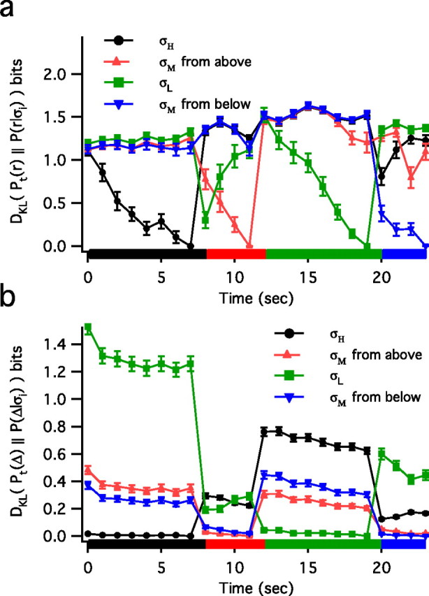
Kullback–Leibler divergence D_KL between the time-dependent distributions and the relevant reference distributions for rate D_KL [P_t(r),P(r|σ_i)] (a) and intervals D_KL [P_t(Δ),P(Δ|σ_i)] (b). Each distribution was created from 1 s (times 300 repeats) of this 24 s stimulus pattern. Reference distributions are sampled from the final second of each of the four epochs, hence D_KL = 0 at 7, 11, 19, and 23 s. Although rate distributions change continuously throughout the epoch (a), interval distributions quickly reach a steady state (b). Error bars represent the SD.

Figures 1d and 2b suggest that information about stimulus variance can be obtained quickly from ISIs after a transition. Therefore, we calculate the time-dependent mutual information provided by each successive interval after a variance switch according to Equation 4 in Materials and Methods. For the nth interval after a switch, Δ_n, we calculate I(Δ_n;σ) and find that the amount of information provided by each interval increases rapidly to a steady state (Fig. 3). Given a three-state discrimination, there is a maximum of log₂(3) = 1.585 bits of information to obtain. If the assumption of independent intervals is valid, perfect discrimination then can be achieved with ∼8–12 intervals.

Evaluating the accuracy and precision of the distributional code

How accurately can such an interval code convey stimulus information, and what are the speed/accuracy tradeoffs in estimating the variance from a sequence of intervals? One expects that the distributions are most discriminable in the steady state and that adaptation will slow the acquisition of information about a variance change. Therefore, we examined steady-state data from the C. vicina fly viewing uniformly distributed white noise motion stimuli with a constant variance and data from a HH model neuron (Hodgkin and Huxley, 1952) driven by a Gaussian-distributed white noise current input with constant variance.

ISI distributions of the fly and simulated data demonstrate a shift of the peak toward shorter intervals, with increasing stimulus variance that is more marked in the fly ISI distributions than in the simulated data (Fig. 4a,b). Although both distributions display tails at long time scales, the tails of the fly ISI distributions have a consistent slope, whereas the relative area under the HH tails increases dramatically with decreasing variance. The presence of these long time scale tails allows for significant changes in spike rate without a large change in the overall ISI distribution. Contours of the Kullback–Leibler divergences between distributions generated from stimuli with SD σ_A and σ_B are plotted in Figure 4, c and d, and the asymmetry in the D_KL is readily apparent because the greatest distance for the fly data is between responses resulting from low- to high-variance switches in contrast to the model neuron in which the opposite is true.

Asymmetry in the discrimination of variance transitions has been noted previously in a fly experiment of time-varying variance, in which steady-state information transmission was reached more quickly after an increase in stimulus variance than after a decrease in variance (Fairhall et al., 2001). In the detection of a variance change in a Gaussian distribution, this asymmetry follows directly from signal detection theory: it is easier to spot an unexpected large-variance outlier than to realize that too many values are falling in the center of the distribution (DeWeese and Zador, 1998; Fairhall et al., 2001; Snippe et al., 2004). Our results, which examine steady-state data, suggest that in decoding the change the opposite also can be true; the interval distributions are highly non-Gaussian, and the direction of the asymmetry in D_KL will depend on the particular shape of the two distributions. For decoding during adaptation at least two asymmetries may compete: different rates of adaptation either can reinforce or can counteract the asymmetry in reading out the non-Gaussian signal from the interval data. Even in steady state there may be two causes of asymmetry: again, the possible asymmetry of the D_KL divergence between distributions (Fig. 4c,d) and an asymmetry in the variance of a discriminator variable, such as the SNR discriminator based on Equation 3. Even when the D_KL is higher for a low-to-high variance transition, a very large variance can make this transition less reliably detected from the resulting intervals than a high-to-low transition (data not shown).

To quantify how well information about stimulus variance can be decoded from sequences of n intervals, we assume successive intervals are independent and use the cumulative D_cKL⁽ⁿ⁾, Equation 2, to compare responses (see Materials and Methods). Figure 5 shows how the estimated D_cKL⁽ⁿ⁾ varies as a function of stimulus SD ratio for several values of n. It is evident that discrimination is relatively easier for the model neuron than for the fly H1 neuron. The asymmetries of Figure 4, c and d, also are reflected here such that discrimination is easier for low-to-high variance changes in the fly data, and high-to-low variance changes are discriminated more easily from model neuron data.

Figure 5.

Cumulative Kullback–Leibler divergence (D_cKL⁽ⁿ⁾) between neural responses, as defined in Equation 2, as a function of the log ratio of two stimulus SDs, σ_B and σ_A. This divergence is related to the probability of misclassification in which a distance of one bit corresponds to a twofold reduction in error and is a measure of the capacity to discriminate between two ISI distributions resulting from two stimulus variances, as in Figure 4, a and b. D_cKL⁽ⁿ⁾ is for n = 1, 3, or 5 ISIs from fly data for a given SD ratio (a) and from the HH model neuron (b). For example, the circle represents the average discrimination for all 10-fold ratios of stimulus SD decrease, e.g., 10 to 1, 30 to 3, and 60 to 6. Error bars represent the SD.

As a measure of discrimination we use a difference of one bit, which corresponds to a twofold reduction in the probability of classification error by a decoder (Johnson et al., 2001). Discriminating stimuli with SDs that differ by a factor of 10 in the fly (Fig. 6a,c) requires approximately three intervals and ∼100 ms. For HH output the discrimination is relatively easier: discrimination of variances differing by a factor of 3 requires approximately three spikes and <100 ms (Fig. 6b,d). Although the time to discrimination typically increases with the number of spikes required, this is not always true and depends on the shape of the ISI distributions. For example, when we compare distributions that differ significantly in the long time scale tails, few spikes may be needed to reach a given level of discrimination, but the average required time may be long if the discriminating spike intervals lie in the long time scale tails.

Figure 6.

Number of spikes and corresponding mean time needed for discrimination, where discrimination is defined as a distance of one bit. For each data series, the stimulus SD of the comparison distribution (σ_A) is held constant while the SD of the source distribution varies (σ_B). a, Number of H1 spikes required to discriminate between two variances. b, HH spikes required to discriminate between two variances. c, Mean time (seconds) in fly H1 neuron required to discriminate between two variances. d, Mean time (seconds) in HH neuron required to discriminate between two variances. Discrimination requires considerably fewer spikes and less time in the model neuron as compared with the fly neuron. The figure key values (right) for σ_A and σ_B are in normalized units of SD, which correspond to those in Figure 4.

Because this measure of decoding ability assumes independence of successive ISIs, we test this assumption in two ways. First, we calculate D_KL values for a two-interval discrimination, using both the joint distribution of the two ISIs, which takes into account interval correlations, and the independent approximation, Equation 3. For the fly data we find that, as expected, discrimination with the joint distribution is slightly better but on the whole very similar (Fig. 7a). Second, we calculate the mutual information I(Δ₁;Δ_n) between the first and the nth interval in a sequence, according to Equation 5, for each of the distributions in Figure 4a and plot their mean values (Fig. 7b). This gives us a measure of the correlations between intervals and is equivalent to the D_KL between the joint and independent distributions of Δ₁ and Δ_n. After a separation of more than one interval, the intervals, although slightly correlated, have very small mutual information and can be considered as approximately independent (Fig. 7b). For the HH neuron there is approximately zero correlation after a single interval.

Figure 7.

Testing the independence assumption. a, Kullback–Leibler divergences calculated by using independent distributions for P(Δ₁|σ) and P(Δ₂|σ) (triangles) and joint distributions P(Δ₁,Δ₂|σ) (circles) as a function of the log ratio of two stimulus SDs, σ_B and σ_A, for independent distributions; error bars represent the SD. b, Mutual information, Equation 5, between the first spike interval and the nth interval of fly data for interval sequences that result from steady-state zero-mean stimuli with varying SDs. The sharp decrease between n = 2 and n = 3 suggests that dependence between intervals is confined mainly to the first and second interval; other intervals effectively are drawn randomly from the probability distribution. This information calculation was corrected for undersampling, as described in Materials and Methods. Gray lines represent the mutual information between intervals from different variance distributions, whereas the black line represents the mean; error bars represent the SD across different stimulus conditions.

Real-time decoding

Until now, we have assessed the ability with which one, in principle, could decode information about stimulus variance. However, we also would like to decode stimulus variance explicitly. Because we have unlimited data from the HH model, we use the simulation to test the plausibility of one-trial real-time decoding of a continuously varying variance envelope. Therefore, we now estimate stimulus variance using one example of a 60 s spike train from the HH neuron (Fig. 8). We assume that we have access to a library of reference distributions P(Δ|σ) in which each distribution is gathered from a steady-state stimulus variance experiment (Fig. 4b). From this we can use a maximum likelihood estimator to estimate the value of the time-varying stimulus variance: the estimate is the SD that yields the highest probability of n successive spike intervals, as in Equation 6. In principle, given a suitable parametric family of distributions as a function of variance, one might compute these results analytically. However, here we use sampled data with 10 values of the variance spaced such that successive variances are ∼1.6 times the previous (given Fig. 5b, this is a reasonable discretization scale for decoding with the use of more than one interval). If we consider two successive intervals, an estimate requires on average 22 ms of spike train data (Fig. 8a), whereas an estimate based on 15 intervals requires a mean time of 314 ms (Fig. 8b). Using these mean times as the window width, we also estimate stimulus SD from the number of spikes in this window. As the number of intervals considered or the window width increases, variance estimates better match the true stimulus variance (Fig. 8c,d). Because the HH model does not display spike frequency adaptation, we do not expect any ambiguity, as exemplified in Figure 1, and estimates from intervals and spike rate should converge for long-enough windows (Fig. 8e). However, calculating spike rate in short windows severely discretizes the possible estimates of variance (Fig. 8a, red circles), and for short times the calculations based on intervals can give better variance estimates even when adaptation is not present (Fig. 8e).

Figure 8.

Decoding a time-varying stimulus SD from HH spike trains by using 2 ISIs (a) and 15 ISIs (b, green lines). For each data point we find σ, for which P(Δ_n|σ) is maximized for either 2 or 15 intervals, as in Equation 6. Stimulus SD is estimated from the rate calculated in a window width equal to the mean time of 2 or 15 intervals (22 and 314 ms, respectively; red circles). The instantaneous stimulus SD is shown in black. At very short times, the range of possible estimates is limited when calculated from rate, but not from intervals. For longer times, the estimates from rate and intervals are comparable, because the HH model does not show slow spike frequency and would not be expected to display the ambiguity between rate and intervals as in fly neuron (Fig. 1). Shown is a comparison of estimated versus true SD, using intervals (c) and spike rate (d), in which the vertical bars represent the SDs of the estimated SD, and mean-squared error of the estimated SD (e) as a function of interval number or spike rate bin width.

Discussion

We have examined the ability of a code based on the local distribution of ISIs to convey information about stimulus variance in an identified fly visual neuron and in a simulated HH neuron. We present a specific example in the fly visual system in which adapting spike rates measured locally give insufficient information to determine stimulus variance, whereas an ISI distributional code allows this discrimination to be performed with reasonable accuracy. We find that this code can be decoded rapidly to convey accurate information about the local stimulus variance, that the precision of this code depends on the particular shape of the ISI distribution, and that this code is effective in the general and simple HH model neuron.

During adaptation in H1 the rate distributions do not provide a unique mapping to stimulus variance, whereas ISI distributions provide an approximately one-to-one mapping (Fig. 1). This results from the observation that rate distributions evolve slowly with time (on the order of seconds), whereas ISI distributions quickly (∼200 ms) reach a steady state (Fig. 2). The ISI distributions permit variance discrimination as quantified by the Kullback–Leibler divergence, which depends on the shape of the ISI distribution (Figs. 4–6). This can lead to asymmetries with respect to variance increases or decreases in the time to decode the variance change. Decoding with ISI distributions can be used to estimate a time-varying stimulus variance (Fig. 8).

As demonstrated in Figures 1–3, this distributional code can yield stimulus variance information quickly that is unavailable from spike rate; qualitatively, this is based on the shapes of the ISI distributions, which reach steady state after a sudden variance change more quickly than does spike rate. That the ISI distributions may be very similar although the spike rate distributions are different and evolving may seem paradoxical, because the firing rate can be defined as the inverse of the mean ISI. However, here we have considered rate computed from spike counts in a given time window. Short intervals are characteristic of a given variance, and variance adaptation leads to a slow change in the proportion of short and long intervals. In the switch to a new variance there is very rapid change in the typical pattern of short intervals, although the relative probability of long intervals adapts more slowly. These small changes in the long interval tails of the distributions lead to significant variations in the rate, as we have observed during adaptation. These features typically render the rate unsuitable to estimate accurately over the short times relevant for the encoding of natural stimuli (Gautrais and Thorpe, 1998). Furthermore, different parts of the interval distribution adapt at different speeds, and we accentuate this feature by plotting log–ISI distributions.

The robustness of this distributional code is related to the shape of the steady-state distributions. The ISI distributions of both the fly H1 neuron and the HH model vary systematically with the variance of the driving stimulus. These variations can be analyzed quantitatively by using the Kullback–Leibler divergences (Figs. 4c,d, 5, 6). It has been noted previously that it is easier, both theoretically and experimentally, to discriminate a variance increase than a variance decrease (DeWeese and Zador, 1998; Fairhall et al., 2001; Snippe et al., 2004). However, here we have considered the speed and accuracy of decoding from a non-Gaussian distribution, where this may not hold. As has been pointed out (DeWeese and Zador, 1998), the speed of recognizing a change in distribution depends on the occurrences of outliers after the change. In our results the distributions corresponding to different stimulus variances have distinct and non-Gaussian forms; Figure 4, a and b, includes cases in which the occurrence of distinctive outliers happens more frequently for the low-variance distribution than for the high-variance distribution, thus resulting in easier identification of the low-variance rather than the high-variance source.

In addition to coding via spike rate, spike timing, and specific spike patterns, distributional coding may provide another means for the neuron to transmit information. Although information in spike rate typically is thought to be transmitted rapidly via averaging across populations of neurons (Shadlen and Newsome, 1998), we have shown that this distributional code provides a means of conveying ensemble information rapidly (∼10–100 ms) via the output of a single neuron. Other results also show a strong dependence of the interval statistics on the variance of the driving stimulus (Johannesma, 1969; Hunter et al., 1998; Wang and Wang, 2000; Hunter and Milton, 2003). Furthermore, results from the HH neuron demonstrate that this variance dependence is present for a simple conductance-based model neuron and is likely to be present for many neural types. The decoding scheme that we propose shows that, in principle, this information is available. A biophysical implementation of such a decoding may involve an array of tuned synapses showing short-term depression and facilitation (Tsodyks and Markram, 1997; Varela et al., 1997) to provide sensitivity to interval sequence. Thus a library of probability distributions P(Δ|σ) (as in Fig. 4b) might be “stored” at synapses in which a preferred ISI sequence leads to a maximal postsynaptic response.

Adaptation is functionally very important for sensory systems, allowing the system to tailor its responses to the local stimulus and thereby increase information transmission. However, adaptation leads to ambiguity, whereby the relationship between stimulus and response is no longer one-to-one but depends on the statistical context of the stimulus. There are three possible solutions to this problem. Information may be conveyed by other neurons in the network, or it may be discarded entirely, as may be the case for light/dark adaptation of photoreceptors. We suggest a third possibility: contextual information may be conveyed by the statistical properties of the spike train. Although the first two of these possibilities also may be true for H1, we have demonstrated that information about the statistical ensemble indeed may be extracted. The dependence of the interval statistics on the stimulus ensemble may be a generic property of neural response, because it is observed in neurons as simple as the HH model (Wang and Wang, 2000). It therefore is tempting to suggest that using this dependence to convey ensemble information may be a universal capability of neural computation.

References

- Baccus SA, Meister M. Fast and slow contrast adaptation in retinal circuitry. Neuron. 2002;36:909–919. doi: 10.1016/s0896-6273(02)01050-4. [DOI] [PubMed] [Google Scholar]
- Bialek W, Rieke F, de Ruyter van Steveninck RR, Warland D. Reading a neural code. Science. 1991;252:1854–1857. doi: 10.1126/science.2063199. [DOI] [PubMed] [Google Scholar]
- Brenner N, Strong SP, Koberle R, Bialek W, de Ruyter van Steveninck RR. Synergy in a neural code. Neural Comput. 2000;12:1531–1552. doi: 10.1162/089976600300015259. [DOI] [PubMed] [Google Scholar]
- Carandini M, Ferster D. A tonic hyperpolarization underlying contrast adaptation in cat visual cortex. Science. 1997;276:949–952. doi: 10.1126/science.276.5314.949. [DOI] [PubMed] [Google Scholar]
- Cariani P. Temporal coding of periodicity pitch in the auditory system: an overview. Neural Plast. 1999;6:147–172. doi: 10.1155/NP.1999.147. [DOI] [PMC free article] [PubMed] [Google Scholar]
- Cover TM, Thomas JA. Elements of information theory. New York: Wiley; 1991. [Google Scholar]
- Dayan P, Abbott LF. Theoretical neuroscience: computational and mathematical modeling of neural systems. Cambridge, MA: Massachusetts Institute of Technology; 2001. [Google Scholar]
- Dean I, Harper NS, McAlpine D. Neural population coding of sound level adapts to stimulus statistics. Nat Neurosci. 2005;8:1684–1689. doi: 10.1038/nn1541. [DOI] [PubMed] [Google Scholar]
- de Ruyter van Steveninck R, Bialek W. Real-time performance of a movement-sensitive neuron in the blowfly visual system: coding and information transfer in short spike sequences. Proc R Soc London B Biol Sci; 1988. pp. 379–414. [Google Scholar]
- DeWeese M, Zador A. Asymmetric dynamics in optimal variance adaptation. Neural Comput. 1998;10:1179–1202. [Google Scholar]
- Egelhaaf M, Warzecha AK. Encoding of motion in real time by the fly visual system. Curr Opin Neurobiol. 1999;9:454–460. doi: 10.1016/s0959-4388(99)80068-3. [DOI] [PubMed] [Google Scholar]
- Fairhall AL, Lewen GD, Bialek W, de Ruyter Van Steveninck RR. Efficiency and ambiguity in an adaptive neural code. Nature. 2001;412:787–792. doi: 10.1038/35090500. [DOI] [PubMed] [Google Scholar]
- Franceschini N, Riehle A, Le Nestour A. Directionally selective motion detection by insect neurons. In: Stavenga DG, Hardie RC, editors. Facets of vision: compound eyes from Exner to Autrum and beyond. Berlin: Springer; 1989. pp. 360–390. [Google Scholar]
- Gautrais J, Thorpe S. Rate coding versus temporal order coding: a theoretical approach. Biosystems. 1998;48:57–65. doi: 10.1016/s0303-2647(98)00050-1. [DOI] [PubMed] [Google Scholar]
- Gelman A. Ed 1. London: Chapman and Hall; 1995. Bayesian data analysis. [Google Scholar]
- Haag J, Borst A. Encoding of visual motion information and reliability in spiking and graded potential neurons. J Neurosci. 1997;17:4809–4819. doi: 10.1523/JNEUROSCI.17-12-04809.1997. [DOI] [PMC free article] [PubMed] [Google Scholar]
- Hodgkin AL, Huxley AF. A quantitative description of membrane current and its application to conduction and excitation in nerve. J Physiol (Lond) 1952;117:500–544. doi: 10.1113/jphysiol.1952.sp004764. [DOI] [PMC free article] [PubMed] [Google Scholar]
- Hunter JD, Milton JG. Amplitude and frequency dependence of spike timing: implications for dynamic regulation. J Neurophysiol. 2003;90:387–394. doi: 10.1152/jn.00074.2003. [DOI] [PubMed] [Google Scholar]
- Hunter JD, Milton JG, Thomas PJ, Cowan JD. Resonance effect for neural spike time reliability. J Neurophysiol. 1998;80:1427–1438. doi: 10.1152/jn.1998.80.3.1427. [DOI] [PubMed] [Google Scholar]
- Johannesma PIM. PhD thesis. The Netherlands: University of Nijmegen; 1969. Stochastic neural activity: a theoretical investigation; p. 91. [Google Scholar]
- Johnson DH, Gruner CM, Baggerly K, Seshagiri C. Information-theoretic analysis of neural coding. J Comput Neurosci. 2001;10:47–69. doi: 10.1023/a:1008968010214. [DOI] [PubMed] [Google Scholar]
- Keat J, Reinagel P, Reid RC, Meister M. Predicting every spike: a model for the responses of visual neurons. Neuron. 2001;30:803–817. doi: 10.1016/s0896-6273(01)00322-1. [DOI] [PubMed] [Google Scholar]
- Kepecs A, Lisman J. Information encoding and computation with spikes and bursts. Network Comput Neural Syst. 2003;14:103–118. [PubMed] [Google Scholar]
- Kim KJ, Rieke F. Temporal contrast adaptation in the input and output signals of salamander retinal ganglion cells. J Neurosci. 2001;21:287–299. doi: 10.1523/JNEUROSCI.21-01-00287.2001. [DOI] [PMC free article] [PubMed] [Google Scholar]
- Kvale MN, Schreiner CE. Short-term adaptation of auditory receptive fields to dynamic stimuli. J Neurophysiol. 2004;91:604–612. doi: 10.1152/jn.00484.2003. [DOI] [PubMed] [Google Scholar]
- Lesica NA, Stanley GB. Encoding of natural scene movies by tonic and burst spikes in the lateral geniculate nucleus. J Neurosci. 2004;24:10731–10740. doi: 10.1523/JNEUROSCI.3059-04.2004. [DOI] [PMC free article] [PubMed] [Google Scholar]
- Mainen ZF, Sejnowski TJ. Reliability of spike timing in neocortical neurons. Science. 1995;268:1503–1506. doi: 10.1126/science.7770778. [DOI] [PubMed] [Google Scholar]
- Meister M, Berry MJ., 2nd The neural code of the retina. Neuron. 1999;22:435–450. doi: 10.1016/s0896-6273(00)80700-x. [DOI] [PubMed] [Google Scholar]
- Paninski L. Estimation of entropy and mutual information. Neural Comput. 2003;15:1191–1253. [Google Scholar]
- Panzeri S, Treves A. Analytical estimates of limited sampling biases in different information measures. Network Comput Neural Syst. 1996;7:87–107. doi: 10.1080/0954898X.1996.11978656. [DOI] [PubMed] [Google Scholar]
- Press WH. Numerical recipes in C: the art of scientific computing. Ed 2. Cambridge, UK: Cambridge UP; 1992. [Google Scholar]
- Reich DS, Mechler F, Purpura KP, Victor JD. Interspike intervals, receptive fields, and information encoding in primary visual cortex. J Neurosci. 2000;20:1964–1974. doi: 10.1523/JNEUROSCI.20-05-01964.2000. [DOI] [PMC free article] [PubMed] [Google Scholar]
- Reinagel P, Reid RC. Precise firing events are conserved across neurons. J Neurosci. 2002;22:6837–6841. doi: 10.1523/JNEUROSCI.22-16-06837.2002. [DOI] [PMC free article] [PubMed] [Google Scholar]
- Rieke F, Warland D, de Ruyter van Steveninck R, Bialek W. Spikes: exploring the neural code. Cambridge, MA: Massachusetts Institute of Technology; 1997. [Google Scholar]
- Shadlen MN, Newsome WT. The variable discharge of cortical neurons: implications for connectivity, computation, and information coding. J Neurosci. 1998;18:3870–3896. doi: 10.1523/JNEUROSCI.18-10-03870.1998. [DOI] [PMC free article] [PubMed] [Google Scholar]
- Shapley R, Victor JD. The contrast gain control of the cat retina. Vision Res. 1979;19:431–434. doi: 10.1016/0042-6989(79)90109-3. [DOI] [PubMed] [Google Scholar]
- Snippe HP, Poot L, van Hateren JH. Asymmetric dynamics of adaptation after onset and offset of flicker. J Vis. 2004;4:1–12. doi: 10.1167/4.1.1. [DOI] [PubMed] [Google Scholar]
- Stanley GB, Li FF, Dan Y. Reconstruction of natural scenes from ensemble responses in the lateral geniculate nucleus. J Neurosci. 1999;19:8036–8042. doi: 10.1523/JNEUROSCI.19-18-08036.1999. [DOI] [PMC free article] [PubMed] [Google Scholar]
- Strong SP, Koberle R, de Ruyter van Steveninck R, Bialek W. Entropy and information in neural spike times. Phys Rev Lett. 1998;80:197–200. [Google Scholar]
- Treves A, Panzeri S. The upward bias in measures of information derived from limited data samples. Neural Comput. 1995;7:399–407. [Google Scholar]
- Tsodyks MV, Markram H. The neural code between neocortical pyramidal neurons depends on neurotransmitter release probability. Proc Natl Acad Sci USA. 1997;94:719–723. doi: 10.1073/pnas.94.2.719. [DOI] [PMC free article] [PubMed] [Google Scholar]
- Varela JA, Sen K, Gibson J, Fost J, Abbott LF, Nelson SB. A quantitative description of short-term plasticity at excitatory synapses in layer 2/3 of rat primary visual cortex. J Neurosci. 1997;17:7926–7940. doi: 10.1523/JNEUROSCI.17-20-07926.1997. [DOI] [PMC free article] [PubMed] [Google Scholar]
- Wang Y, Wang ZD. Information coding via spontaneous oscillations in neural ensembles. Phys Rev E Stat Phys Plasmas Fluids Relat Interdiscip Topics. 2000;62:1063–1068. doi: 10.1103/physreve.62.1063. [DOI] [PubMed] [Google Scholar]
- Warland DK, Reinagel P, Meister M. Decoding visual information from a population of retinal ganglion cells. J Neurophysiol. 1997;78:2336–2350. doi: 10.1152/jn.1997.78.5.2336. [DOI] [PubMed] [Google Scholar]