Spike Count Reliability and the Poisson Hypothesis

Abstract

The variability of cortical activity in response to repeated presentations of a stimulus has been an area of controversy in the ongoing debate regarding the evidence for fine temporal structure in nervous system activity. We present a new statistical technique for assessing the significance of observed variability in the neural spike counts with respect to a minimal Poisson hypothesis, which avoids the conventional but troubling assumption that the spiking process is identically distributed across trials. We apply the method to recordings of inferotemporal cortical neurons of primates presented with complex visual stimuli. On this data, the minimal Poisson hypothesis is rejected: the neuronal responses are too reliable to be fit by a typical firing-rate model, even allowing for sudden, time-varying, and trial-dependent rate changes after stimulus onset. The statistical evidence favors a tightly regulated stimulus response in these neurons, close to stimulus onset, although not further away.

Introduction

The variability of spike trains bears on theories of neural coding. A range of hypotheses have been offered. At one extreme, the existence and precise temporal location of every spike is significant. At another extreme, a spike train is a stochastic process essentially characterized by a slowly changing rate. The latter hypothesis leads naturally to modeling spikes as the events of a slowly varying inhomogeneous Poisson process (the “Poisson hypothesis”). Fine-temporal coding would be more likely to yield highly regular spike counts from repeated trials, whereas randomness in the Poisson hypothesis limits the degree of regularity across trials.

A statistic commonly used to assay variability in spike trains is the empirical variance/mean ratio of the spike counts (the Fano factor) across trials (Tolhurst et al., 1983; Softky and Koch, 1993; Shadlen and Newsome, 1998; Oram et al., 1999; Kara et al., 2000). For example, the spike counts for the inhomogeneous Poisson process are distributed as a discrete Poisson random variable, for which the mean and variance are identical. By this measure, the spike counts of in vivo cortical spike trains (in contrast perhaps to subcortical structures) have generally been thought to be as variable as Poisson processes and perhaps even more so (Shadlen and Newsome, 1998; Koch, 1999). As Shadlen and Newsome (1998) have written, “When an identical visual stimulus is presented for several repetitions, the variance of the neural spike count has been found to exceed the mean spike count by a factor of 1–1.5 wherever it has been measured.”

Inferring a lack of precision in the neural code from observations of variability is tricky. One line of reasoning is that the existence of variability under identical conditions, when the neuron is presumably signaling the same event, reflects noise (e.g., Poisson noise) in the signaling process itself. However, it is certainly plausible that a significant source of variability is the experimenter's own uncertainty about hidden contextual variables that the neuron is encoding (and that may be, for example, internal to the brain), such as attention, or the states of other neurons. Furthermore, the variability of overt behaviors that are difficult, but not impossible, to measure, like precise eye position, have been shown to contribute to at least some of the variability commonly reported in cortical responses (Gur et al., 1997). As Barlow wrote about neural responses in 1972, “their apparently erratic behavior was caused by our ignorance, not the neuron's incompetence.”

Regularity, in contrast, cannot be explained away so easily, and in this light, evidence of finer temporal structure, particularly in higher-order cortical areas, is intriguing. Recently, Muller et al. (2001) have observed, from recordings of V1 cells in primates presented with sinusoidal gratings, that near stimulus onset, the empirical variance/mean ratio is strikingly smaller than unity (in apparent contradiction to the Poisson hypothesis). This is in line with other reports that suggest a greater reliability in cortical responses than might be expected from a Poisson model (Gur et al., 1997; Gershon et al., 1998; Kara et al., 2000).^a

Our purpose in this paper is twofold. First, we derive a simple and exact test for a “minimal Poisson hypothesis” that uses the variability of spike counts across trials. The minimal Poisson hypothesis includes Poisson processes that have rapidly (in fact arbitrarily) changing spiking rates, possibly differing from trial to trial. Second, we present evidence consistent with these previous studies of low variance/mean ratios, particularly near stimulus onset, gathered here in cells from anterior inferotemporal (IT) cortex of primates presented with more complex visual stimuli. Using this test on the IT recordings, we are able to reject the minimal Poisson hypothesis, with a notably small amount of data, predominantly near stimulus onset. We are able to argue, furthermore, that these results are not likely to be attributable to the effects of refractory period per se, but rather reflect regularity in the neural response.

Materials and Methods

Subjects and materials. The basic behavioral and surgical methods used in this study have been described previously (Sheinberg and Logothetis, 1997, 2001). In brief, after initial behavioral training, two rhesus monkeys underwent aseptic surgery for the placement of a head restraint and a scleral search coil. All surgical procedures were performed in accordance with the National Research Council Guide for the Care and Use of Laboratory Animals. After surgery, the monkeys were trained to fixate on a small yellow spot [0.25 degrees (deg)] appearing in the center of a computer monitor. After acquiring the spot, between three and five visual images, 4 deg on a side, were flashed behind the spot for either 800 or 1100 ms. Interstimulus intervals (during which only the spot was visible) were set to the same duration as the stimulus presentation duration (Fig. 1). Visual stimuli were selected from a set of commercially available stock photographs of animals, natural scenes, and man-made objects (Corel, Ottawa, Ontario, Canada).

Figure 1.

Basic fixation task performed by the monkeys. In a single observation period, between three and five individual visual stimuli were flashed on and off as the monkey fixated on a spot in front of the images. At the end of the trial, the monkey received a juice reward for reacquiring the spot as it jumped from the center of the screen to one of four randomly selected peripheral locations.

During stimulus presentation, the monkeys were required to maintain fixation within a virtual square region 2 deg on a side. During data collection, the digitized eye position was stored to disk every 5 ms (200 Hz). In addition to keeping their gaze directed within the virtual window, the monkeys learned to follow the spot as it jumped from the center of the display to a new position. On refixation of the spot, they were rewarded with a drop of apple juice.

Single cell recordings. Once the animals were trained in the fixation task, a ball and socket chamber housing an 18 gauge guide tube was placed directly above the anterior temporal lobes (anteroposterior, +18; mediolateral, +19). Single unit recordings were made by lowering glass-coated platinum–iridium electrodes by microdrive (Kopf Model 650; David Kopf Instruments, Tujunga, CA) into the lower bank of the superior temporal sulcus and the lateral convexity of the inferior temporal gyrus, just posterior to the anterior middle temporal sulcus. The neural signal was amplified using a BAK Electronics (Germantown, MD) A-1 amplifier with remote head stage, and the conditioned signal was fed into a time-amplitude window discriminator. Individual cells were isolated while the animals performed the fixation task. Each cell was tested with at least eight stimuli, but often with many more (≤80). Note that a significant effort was made to subselect visual stimuli from the relatively large test set that effectively elicited robust neuronal responses, as judged by online rasters. Furthermore, we restricted the data analysis only to recordings of neuronal activity characterized by high signal-to-noise ratios, indicating high single-unit isolation quality (Fig. 2).

Figure 2.

Analog voltage trace of neuronal activity from a single trial from one of the recordings used in the analysis. The high signal-to-noise ratio here is typical of the units used in this study.

A statistical test for minimally Poisson spike trains. Consider a series of spike trains from a single neuron obtained from n separate trials (each involving, for example, presentation of the same stimulus):, where there are m_j spikes in trial j, and is the time of occurrence of the ith spike in the jth trial, relative to a stimulus onset at time 0.

A homogeneous Poisson process of rate λ is a statistical model of the spike train that is characterized by two conditions: (1) the events in nonoverlapping time intervals are independent, and (2) the expected number of spikes in a time interval of length T is λT. An inhomogeneous Poisson process is the nonstationary analog of this: events in nonoverlapping time intervals are independent, but the expected number of spikes is governed by a time-varying rate λ(t). An implication of these assumptions, for both homogeneous and inhomogeneous Poisson processes, is that the total number of spikes in any time interval is distributed as a Poisson random variable.

The mean μ and variance σ² of any Poisson random variable are identical, and therefore, the variance/mean ratio σ²/μ, called the Fano factor, is equal to one. Perhaps for this reason, the Fano factor is used frequently in neuroscience as a rate-controlled measure of the reliability of spike counts of neural responses.

The mean μ and variance σ² must be estimated from data. Usually, the empirical statistics are used:

(1)

[Here, we use to signify the estimate of μ, et cetera; see Kass et al. (2004), for an introductory overview of statistical concepts in the context of neuroscience.] The estimates and will converge in a sense of probability to the correct distributional quantities, μ and σ², as the number of trials n increases, provided that m₁,..., m_n are independent and identically distributed.

Typically the Fano factor and Poisson standards are evaluated by comparing the relationship between the empirical mean and the empirical variance of spike counts across a population of neurons and response conditions. This is done visually with a scatter plot and/or analytically, either by fitting a population of estimated mean and variance pairs () to a power law and examining the fitted coefficients, or by reporting the average of empirical Fano factors across a population [for some representative examples, see McAdams and Maunsell (1999), Berry et al. (1997), Buracas et al. (1998), Gur et al. (1997), and Muller et al. (2001)]. Thus, estimated quantities (i.e., the estimated mean , estimated variance , and estimated Fano factor ) are treated interchangeably with their associated distributional quantities (i.e., the mean μ, variance σ², and Fano factor σ²/μ of the distribution presumed to generate the data). This poses fewer problems when these quantities are used solely for comparative analysis [for example, to compare the responses of different classes of neurons (Kara et al., 2000) or different stimulus conditions (McAdams and Maunsell, 1999)], particularly when nonparametric methods are used. As an evaluation of the Poisson model, however, ignoring the sampling variability of these estimators could potentially introduce approximation error into the final conclusions. Standard descriptions of methodology (Teich et al., 1997; Gabbiani and Koch, 1998; Koch, 1999; Dayan and Abbott, 2001) do not discuss or account for this source of error.

Such issues are moot if there are no such true distributional quantities, as when the assumptions that postulate such quantities are not valid. Thus, although we do address this aforementioned gap, the issue of sampling variability is not our major concern here. Rather, we are concerned with the assumption that, even under identical experimental conditions, the responses of a neuron can be reasonably modeled as repeatable quantities. Indeed, the bulk of statistical theory and methods applies to sequences of observations that can reasonably be modeled as identically distributed. It is therefore not surprising that the bulk of applications of statistics to neurophysiological data are made under the assumption, sometimes implicit, that repeated measurements from the same neuron or collection of neurons under the same experimental conditions produces a sequence of identically distributed observations. Thus, a large value for the Fano factor (Shadlen and Newsome, 1998; Koch, 1999; Kara et al., 2000, and references therein; Dayan and Abbott, 2001) is surprising and meaningful only in proportion to our willingness to believe in the proposition of trial-to-trial statistical stationarity. Similarly, sophisticated point-process models of spike trains that accommodate inhomogeneous firing rates and/or spike-to-spike dependencies (Berry and Meister, 1998; Kass and Ventura, 2001) are useful in proportion to our ability to estimate time-varying rates and other high-dimensional parameters. Yet, in the absence of statistically repeatable observations, the estimation of such quantities is difficult and even raises issues of identifiability.

Given the magnitude of unknown and unmeasurable internal and external variables, assumptions of repeatability warrant concern. We derive here an exact statistical test of the Poisson nature of the spike train process, broadly defined, that makes no assumption about trial-to-trial stationarity and even allows for some measure of trial-to-trial statistical dependence (see Results, Derivation of the minimal Poisson variability test). On these terms, one could hardly expect to find a test that gives evidence for excess variability in the spike-generation process. However, it is possible to reject a broad class of models in the direction of excess regularity without appealing to an assumption of trial-to-trial stationarity. Loosely speaking, allowing for additional variability in the form of trial-to-trial variation does not make observations of regularity any less surprising.

Our null hypothesis (H₀) is that m₁, m₂,..., m_n, are independent (but not necessarily identically distributed) Poisson random variables. This is a minimal Poisson hypothesis in the sense that it contains, as a special case, the hypothesis that the recordings come from independent, possibly inhomogeneous, and possibly differing from trial to trial, Poisson processes.

Below, we will derive the following exact statistical test, the “Poisson variability test,” for H₀:

. (2)

The critical value, f(n, α, ), can be explicitly computed and tabulated (Amarasingham, 2004). However, in practice, the actual significance of a given data set is more to the point: for each n (number of trials), N (total number of spikes, ), and S (the statistic, ), we compute the p value α(n, N, S), which is the lowest probability at which the Poisson variability test rejects the null. p values can be computed exactly by dynamic programming or approximately by Monte Carlo sampling. ^b Dynamic programming is computationally feasible for smaller values of N and S and was used in all of the experiments reported here. The Monte Carlo approach is feasible in essentially any situation and has the virtue of simplicity, as is evident from the code listing provided in Appendix A. One needs to choose the number of Monte Carlo samples to be consistent with the desired accuracy, but this requires only a simple application of the binomial distribution. As a benchmark, 10,000 Monte Carlo samples yield an α value with a 95% confidence interval no larger than ± 0.01. Matlab code for running either or both algorithms is available for download at http://www.dam.brown.edu/ptg/REPORTS/amarasingham/pvt.html, as is a copy of Amarasingham (2004), which contains a complete discussion of both algorithms.

Under the constraint , the sum of squares is smallest when the counts m₁, m₂,..., m_n are most nearly equal. This is in fact a corollary of the more familiar statement that the variance measures the “spread” of a distribution, because

(3)

Therefore, the test has power toward alternative hypotheses that would predict more repeatable observations of spike counts than the minimal Poisson hypothesis.

Results

Derivation of the minimal Poisson variability test

Recall that the null hypothesis (H₀) is that m₁, m₂,..., m_n are independent Poisson random variables. Let us designate the (unknown) means as λ₁, λ₂,..., λ_n. Define the empirical mean and variance statistics as usual:

(4)

A hypothesis test specifies a region of the space of outcomes (called the critical region), which is unlikely for all distributions in the null hypothesis. The null hypothesis is “rejected” when observations fall in the critical region. The power of a test with respect to an alternative distribution is the probability that the alternative distribution assigns to the critical region, i.e., the probability that the null hypothesis is rejected when the alternative is true. We seek a hypothesis test under our null, which has higher power for alternative distributions in which (i.e., the empirical Fano factor) tends to be small, or more to the point, such that is small, given . It is equivalent to use in place of , because they preserve the same order when is fixed.

One way to proceed is to form a partition of the sample space based on . We seek f(n, α, ), such that

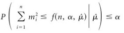(5)

for all and for all P ϵ H₀. Then, the event will be an α-level hypothesis test, because

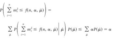(6)

for all P ϵ H₀. To derive f(n, α, ), it is straightforward to apply the following proposition.

Proposition

If m₁, m₂,..., m_n are independent Poisson random variables with means λ₁, λ₂,..., λ_n, respectively, then for all r, and for all , we have the following:

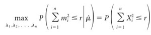, (7)

where X₁, X₂,..., X_n are distributed multinomially with parameters {; 1/n, 1/n,..., 1/n}.

A multinomial distribution generalizes the binomial distribution to a many-sided die and has the following form:

(8)

where p₁, p₂,..., p_n satisfy p_i ≥ 0 and . In shorthand, X₁,..., X_n ∼ M(N; p₁, p₂,..., p_n). This proposition arises from the following observation: conditioned on , the average number of spikes, the counts m₁, m₂,..., m_n are distributed multinomially with the following parameters:

(9)

That is, if the firing rates λ₁, λ₂,..., λ_n and the total spike count are known, one could sample from the minimal Poisson model by assigning each of the spikes to a trial based on the outcome of an n-sided die on which each face is biased in proportion to the firing rate (λ_i) of the trial to which it corresponds. This lends itself to the conjecture that the empirical variance of the m_i, conditioned on , is most likely to be large exactly when the n-sided die is unbiased. (An unbiased die is one that produces all sides with equal likelihood). We formalize this with the proposition, which is not difficult to prove. The proof and other technical details are contained in Amarasingham (2004).

Thus, if

(10)

where X₁,..., X_n ∼ M (; 1/n, 1/n,..., 1/n), then, in light of Equations 5, 6, and 7, {} is an α-level hypothesis test for H₀.

In practice, the interest is in the p value, given an observed value of . For example, if, over four trials one observes spike counts of {2, 3, 1, 4}, then , and one needs to compute , where X₁, X₂, X₃, X₄ ∼ M(10; 1/4, 1/4, 1/4, 1/4). One straightforward way to do this is by simulation (a so-called Monte Carlo approximation): simulate these multinomially distributed random variables several times and count the proportion of times in which the sum of squares of the simulated random variables is ≤30 to approximate . This simple algorithm is expressed in Matlab code in Appendix A.

A careful reading of the derivation above indicates that the Poisson variability test covers a somewhat more general null hypothesis: m₁, m₂,..., m_n are conditionally independent and Poisson distributed, given the Poisson means λ₁, λ₂,..., λ_n (see Appendix B). Thus, the null hypothesis includes the following: (1) the standard model of inhomogeneous Poisson processes with a fixed rate function across trials (this is the case λ₁ = λ₂ =... = λ_n) and (2) trial-varying inhomogeneous Poisson processes (as stated above), but also (3) processes in which a particular inhomogeneous rate function is chosen from an ensemble of possible rate functions for each stimulus presentation, randomly, but not necessarily independently.

Analysis of cell recordings

Our interest in the trial-to-trial variability of inferotemporal cells emerged as a consequence of the simple impression that, given an appropriate stimulus, neuronal responses at least seemed reliable, especially near the onset of the stimulus (Fig. 3). Given the common view that cell firing patterns throughout cortex are invariably irregular, we set out to more rigorously explore this issue.

Figure 3.

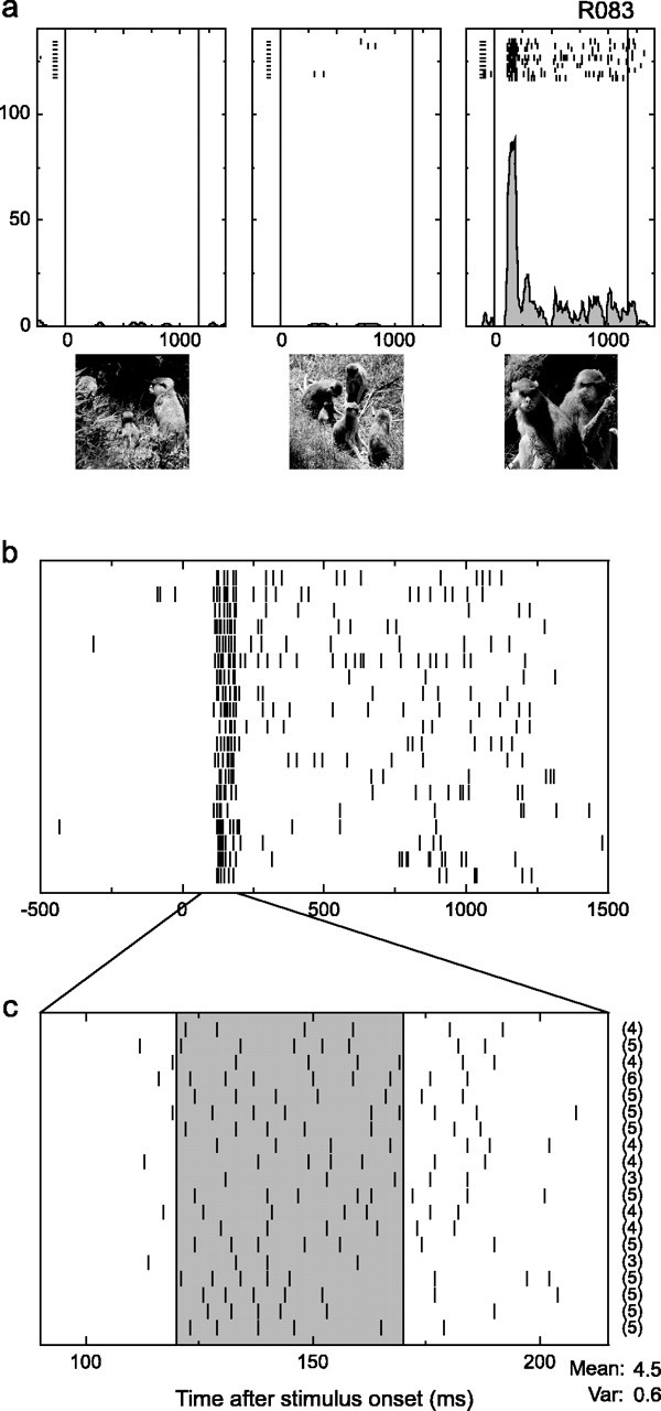
Reliable response from a single cell, indicating that particular stimuli can elicit highly regular trial-to-trial spike discharges from a neuron. a, Response to three of the stimuli used during testing of this cell. Each plot includes the spike rasters aligned to the onset of the stimulus (time indicated by the left vertical line). At the bottom of each plot is an estimate of the instantaneous firing rate. b, Enlarged view of the aligned spike times for all responses to the most effective stimulus shown in a (taken from two separate blocks). c, A temporally expanded view of the spiking activity near stimulus onset, with the number of spikes occurring in the 50 ms shaded area indicated to the right of each trial. Note that the mean of the counts far exceeds the variance (Var) of the counts (ratio, 7.6 times).

To tease apart the effects on variability of time after stimulus onset, we divided the neural response into epochs, consisting of disjoint equal-length time intervals, beginning 100 ms after the onset of presentation of a stimulus. We used intervals of 100 and 50 ms in the experiments described below. These choices were made for empirical reasons and not because of limitations imposed by the test, which can be used for time periods of any length. The pairing of a cell and a stimulus presented repeatedly to the cell we labeled a cell–stimulus pair. For a fixed epoch, associated with each particular cell–stimulus pair are the data points m₁, m₂,..., m_n of spike counts for each of the n presentations of the stimulus to that cell during the epoch. For each cell–stimulus pair, m₁, m₂,..., m_n, (in particular, the statistics and ), determine the p value, the minimal value of α that the Poisson variability test will reject, which we compute as per above.

We analyzed 328 cell–stimulus pairs, drawn from recordings from a total of 27 cells (18 from the first monkey and 9 from the second). These cells were selected on the basis of their clear visual response to at least one visual stimulus and based on the quality of the single unit isolation, which was as high as possible to prevent the uncertainty introduced by a noisy signal from contaminating our data. The number of presentations n varied with each cell–stimulus pair, ranging from n = 2 to n = 14, with a median value of 7.

Using 100 ms epochs, 47 of the 328 pairs were rejected by the Poisson variability test at a significance level of 5% in the 100–200 ms period after stimulus onset. In contrast, the number of rejected cell–stimulus pairs decreased rapidly and progressively at subsequent epochs, further away from onset: 19 rejected pairs between 200 and 300 ms, 11 rejected pairs between 300 and 400 ms, and fewer further on. Similar trends are evident for 50 ms partitions, as illustrated in Figure 4.

Figure 4.

Summary of the rejections from the Poisson variability test across a total of 328 cell–stimulus pairs for each epoch. The 800 ms after stimulus onset were partitioned into disjoint intervals of equal length called epochs. Epochs are labeled along the x-axis by the starting time of the interval with which they are associated. The first row (a, b) summarizes the results from the 100 ms epoch partition, and the second row (c, d) summarized the results from the 50 ms epoch partition. The first column (a, c) illustrates the total number of rejections versus epoch. The second column (b, d) graphs the epoch-by-epoch significance of the number of rejections of the Poisson hypothesis, toward excess regularity, under the assumption that the results of the individual cell–stimulus pair tests are independent. For the first three 100 ms epochs (100, 200, and 300 ms; first 3 bars, first row, second column) the significances are 10^–33, 10^–9, and 10^–3, respectively. For the first four 50 ms epochs (100, 150, 200, and 250 ms; first 4 bars, second row, second column) the significances are 10^–15, 10^–23, 10^–10, and 0.0008, respectively.

Pooling of results

It would not be unexpected for a drug that has no effect to nevertheless show a “significant benefit” in 3 of 100 separate trials, if, say, α = 0.05. After all, even if the null hypothesis is true, we can expect to reject it an average of 5 of 100 times when α = 0.05. How surprising, then, are the number of rejections in each of the tested epochs? One way to assess the significance of the pooled data, within an epoch, is to assume the validity of the null hypothesis and the independence of the tests: the probability of any given number of rejections is then governed by the binomial distribution with parameter p = α. However, in the case of the Poisson variability test as applied here, this is too conservative. In fact, because the statistic is an integer, and because of the small numbers of samples involved in many of these tests, the actual probability of rejecting the null, when the null is true, can be substantially less than α (where α is used to determine the critical value f), and in some cases even zero.

One possible approach to this problem is to include only data with a high number of samples. For example, repeating the analysis described above, but including only the 45 cell–stimuli pairs with at least 10 presentations (i.e., n ≥ 10), we obtain 15 rejections of 45 cell–stimulus pairs in the 100–200 ms epoch, 2 rejected pairs in the 200–300 ms epoch, 4 rejected pairs in the 300–400 ms epoch, and 0 rejected pairs for all subsequent epochs. This approach is conservative, too, however, as any selection of a minimal threshold for the number of samples will be arbitrary: spike counts can still exhibit a surprising amount of regularity even with a few samples.

A better approach is to account for the actual significance values associated with individual tests as a function of sample size. Code for computing the actual significance levels is available at http://www.dam.brown.edu/ptg/REPORTS/amarasingham/pvt.html. Taking this into account, we can compute exactly the distribution on the number of rejections as a sum of Bernoulli (reject/accept) variables with rejection probabilities given by the actual significance levels (Amarasingham, 2004). This gives the exact significance of the observed number of rejections. When applied to the data, this pooling method reveals a consistent trend: the significance of the number of rejections is very high for the 100–200 ms period (significance, 10^–33) and decreases rapidly at subsequent epochs. This and a similar trend for the 50 ms partitions are also illustrated in Figure 4.

Refractory period

One of the most natural biophysical objections to Poisson models of neural activity is the refractory period (Berry and Meister, 1998), which, among other things, introduces strong short-term dependencies in spike train structure (“absolute refractory period”). A statistical test that is sensitive to reliability in the spike counts may merely reflect such local structures (or even not-so-local structures, as in the “relative refractory period”), particularly among cell–stimuli pairs with relatively high firing rates, because the effect of the refractory period on reliability will increase with the firing rate. Indeed, Kara et al. (2000) argue that, in retina, lateral geniculate nucleus, and V1, low spike count variability relative to the Poisson process is primarily explained by absolute and relative refractory periods. One way to examine this interpretation for our data is to compare the results of the variability test across epochs, among cell–stimuli pairs that have the same mean spike counts. If the observed (super-Poisson) reliability is essentially attributable to the refractory period or another interactive effect imposed on an “otherwise” Poisson process [e.g., a Poisson-refractory process, perhaps of the type proposed by Kass and Ventura (2001)], then all other things being equal, one would expect the effect to be independent of the time of occurrence relative to stimulus onset. Figure 5 provides a scatter plot of firing rate versus p value, for cell–stimulus pairs separated by epoch. Although there is a potential refractory period effect manifested by high firing rates near stimulus onset (the proportion of significant pairs grows along the x-axis in the first epoch), this is not enough to explain all of the trends in the data. For a given window of firing rates (e.g., 40–60 Hz), the fraction of significant cell–stimulus pairs is highest in the first epoch (100–200 ms) than in later ones. There is evidently a systematic effect of epoch on spike count reliability, which is independent of firing rate and which cannot be explained by refractory period alone.

Figure 5.

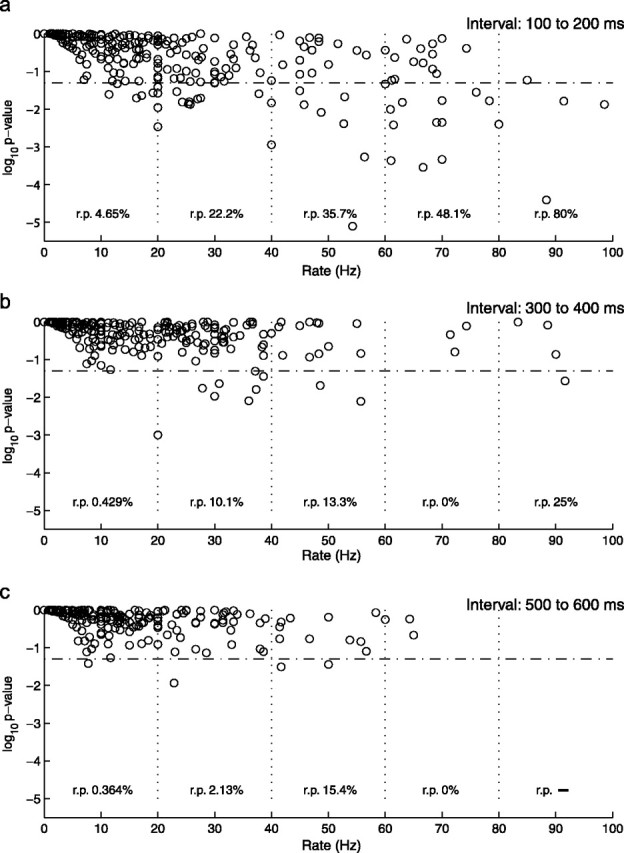
A scatter plot of log₁₀ p value versus firing rate in hertz, across all cell–stimulus pairs, separated in 100 ms epochs. The horizontal dashed line is the line of 5% significance (log₁₀(0.05) ≈–1.301). The firing rate dimension was partitioned into subintervals of 20 Hz range (depicted by the vertical dotted lines), and the proportion of cell–stimulus pairs for which the minimal Poisson hypothesis was rejected [rejection proportion (r.p.)] is provided. The data are plotted separately for the 100–200 ms epoch (a), the 300–400 ms epoch (b), and the 500–600 ms epoch (c), with respect to stimulus onset. (Note that no particular meaning is attached here to the choice of 20 Hz partitions.)

Effect of eye position

In an attempt to more carefully characterize the variable response observed in primary visual cortical cells, Gur et al. (1997) found that the use of moving stimuli coupled with precise control of stimulus position on the retina lowered the variance-to-mean ratio compared with previously reported values. In the present experiment, we did not reposition the stimulus in real time, but we did record eye position throughout each trial. Figure 6 shows one measure of the variability attributable to eye movements during our task, by plotting the SD of the monkeys' horizontal and vertical eye position as a function of time. In general, the variability at each time point was quite low (<0.25 deg), but there is a notable increase in this variability starting ∼300 ms after the stimulus appeared. Even during periods of controlled fixation, eye movements are not completely abolished, and therefore, we cannot rule out the possibility that increased positional uncertainty contributed to higher variability in later temporal epochs.

Figure 6.

Eye position variability. The average SD of both horizontal and vertical eye position for the 800 ms period after stimulus onset indicates that, although there was relatively little positional uncertainty, the variability did increase later in the trial, and this may have contributed to variability later in the neuronal response.

Discussion

Interpreting reliability and variability in neuronal responses

There is an asymmetry in the implications of reliability versus variability in neural responses. Reliability is the more revealing of the two phenomena. For example, suppose that the outputs of a neuron encode information by a temporally reliable spiking process, which would, in turn, imply reliability in the spike counts. Then, provided that the variable being encoded is kept constant or under control in repeated experimental trials, we would expect to observe spike count reliability in observations of the output of that neuron. If it is not held under control, however, we might observe variability in the spike counts through the variation of the unknown encoding variable alone. Thus, under a temporally reliable coding hypothesis, an observation of spike count reliability provides the experimentalist with an additional clue that the neuron is actually encoding something that is being held under experimental control. The clue of reliability can usefully operate in addition to, or even separately from, that of elevated firing rates, which is the chief means by which hypotheses concerning encoded variables are evaluated in neurophysiology. Observations of variability, in contrast, are subject to multiple explanations: either a reliable coding hypothesis is invalid, or the encoded variable is not being held under experimental control. These latter two alternatives, in the case of observed variability, will be quite difficult to distinguish.

This has implications for how we interpret observations of reliability and variability in the neural records. At one extreme, Poisson-like or super-Poisson variability in spike counts is simply accepted as a general principle, and models have been developed to explain this variability. For example, Shadlen and Newsome (1998) postulate mechanisms of synaptic integration designed specifically to preserve the response variability of neurons from one processing stage to the next, motivating this as one of the key features to be explained in cortical physiology.

Based on our data, we suggest that all cortical neurons should not be characterized as a static, homogeneous population with regard to variability of spike discharge. The rejection of the minimal Poisson hypothesis reported here does not imply that all cortical cells exhibit high reliability, only that some apparently do under some, particular, conditions. Many authors have remarked on the potential utility of reliable responses, particularly in the context of neural coding, and so identifying the conditions that generate them suggests itself as an important research topic. One interesting possible scenario is that the reliability of the discharge of a cell is state dependent. Levels of attention or motivation, for example, which are known to affect the firing rate of a cortical cell (for review, see Reynolds and Chelazzi, 2004) and to alter levels of neuronal synchronization (Fries et al., 2001), may also influence the variability of neural response.

Behavioral relevance

The present data were collected under conditions in which the recorded neural signal was in no obvious way related to the animals' behavior. However, numerous previous studies have demonstrated the importance of inferotemporal cortex in successful execution of complex pattern recognition tasks (Logothetis and Sheinberg, 1996). The speed with which monkeys can perform these tasks is of special interest, because they give some hints as to when, and for how long, neuronal signals emanating from IT cortex may be integrated to drive recognition behaviors. Using stimuli similar to those used in this study, for example, Vogels (1999a) found that monkeys could accurately categorize tree and nontree stimuli in <300 ms. More recently, we found that highly similar complex visual images could be discriminated by button response in ∼425 ms but that clear evidence for stimulus identity was evident in the monkeys oculomotor behavior ∼200 ms after stimulus onset (D. L. Sheinberg, unpublished observations). This upper bound of 200 ms is intriguing because it leaves little time for extensive averaging of highly variable signals. Indeed, the average onset latency of selective neuronal responses in IT cortex falls somewhere between 100 and 140 ms (Perrett et al., 1982; Vogels, 1999b; Sheinberg and Logothetis, 2001). Thus, the temporal epoch between initial IT cell activation and discriminatory motor response is quite short, on the order of 100 ms or less. Interestingly, it is precisely during this epoch where we find that individual neurons are most likely to respond reliably to particular visual stimuli.

Models

Identifying models that usefully capture the variability of a cortical spike train remains a central problem in the statistical modeling of neural data. A commonly invoked model is the slow-varying inhomogeneous Poisson process, which follows in a natural way from a rate-coding viewpoint (Shadlen and Newsome, 1998): the signal embedded in a neural spike train is an underlying rate, varying on coarse time intervals on the order of tens to hundreds of milliseconds, and hence, the precise placement of spikes is random and irrelevant. Poisson processes arguably underly a majority of the descriptive and analytic techniques still being used in neural data analysis.

Nevertheless, several studies speak to the inappropriateness of inhomogeneous Poisson models for spike trains (Kass et al., 2004). One explicit reason for this involves short-term dependencies between spikes, as imposed by biophysical phenomena such as the refractory periods and bursting. However, non-Poisson behavior on such fine timescales does not necessarily imply that the spike counts on coarser timescales are not well approximated by a Poisson process. At issue are conclusions of the form exemplified in Koch (1999) (Dayan and Abbot, 2001): “[These results] support the hypothesis that once the refractory period is accounted for, a Poisson hypothesis constitutes a first-order description of cortical spike trains.” Similarly, Kara et al. (2000) argue that much of the super-Poisson reliability that they report, via a Fano factor analysis, might be accounted for by refractory effects, which are differentially affected by varying firing rates. In contrast, our rejection of the minimal Poisson hypothesis is not easily explained by a simple (time-independent) refractory period combined with an otherwise Poisson process, at least in the absence of other forms of regularity in the firing rate, because the rejection occurs near stimulus onset and not further away even among populations of cell–stimulus pairs with similar average firing rates.

Another objection to standard inhomogeneous Poisson models arises from the implicit assumption of statistical stationarity across trials. The typical Fano factor analysis provides one example of such an assumption. The relation of the Fano factor to inhomogeneous Poisson processes, even as a heuristic, requires that there be no variability across trials in the parameters of the process being observed. Such an assumption is the norm in neural data analysis, yet in its absence the significance of many widely used descriptive statistics, such as the peristimulus time histogram, the coefficient of variation, and autocorrelograms and cross-correlograms, is unclear, at best.

Avoiding assumptions of trial-to-trial stationarity requires a more delicate approach. The Poisson variability test is one example. Another example arises naturally in reconstruction paradigms (Brown et al., 1998; Zhang et al., 1998; Brockwell et al., 2004; Wu et al., 2004; Shoham et al., 2005), in which the relationship between behavioral or external variables and the firing rate are explicitly encoded in a model. Once fitted to data, such models can be used to predict, or reconstruct, the behavioral variables from the spike times. However, evaluating the validity of Poisson spike count models by model fitting (Brown et al., 1998, 2002; Shoham et al., 2005) requires that the postulated firing rate models are valid and that their parameters have accurately been estimated. Justifying such an assumption will often be difficult. In particular, conclusions of excess variability (Brown et al., 1998; Fenton and Muller, 1998) can perhaps always be attributed to the effects of additional variables that have not been modeled.^c

In this light, a rejection of the minimal Poisson null hypothesis is unusual because it does not only demonstrate that a single model is not a good fit to the data, but that an entire class of models is inappropriate.

From a pedagogical point of view, the rejection of a null hypothesis implies only that: the rejection of a hypothesis. It does not identify an alternative. However, the form of the statistical test and, in particular, the distribution of its power among the space of alternative hypotheses, may shed light on the data-generating process. The Poisson variability test is based on a measure of the reliability in the spike counts, and hence the rejection of the minimal Poisson hypothesis suggests that the spike train near stimulus onset may be a finely structured temporal process with high precision on many or most of the spikes.

In any case, there is strong statistical evidence that neuronal responses near the onset of a stimulus cannot in general be well modeled by a simple Poisson process, even allowing for a rate function that varies from trial to trial or exhibits transients and other time-dependent activity.

Small samples

The statistical significance of the results is somewhat surprising in light of the small sample sizes, ranging from 2 to 14 per cell–stimulus pair. Indeed, as mentioned previously, some of the observations are so small that rejection of H₀ at 5% significance is mathematically impossible. For example, even if every 100 ms poststimulus epoch had exactly two spikes (corresponding to the most reliable outcome at 20 Hz), the Poisson variability test would only achieve 5% significance with four or more trials. In fact, to take one example, based on the numbers of trials and numbers of observed spikes in the analysis of the 100–200 ms epoch, for 50% of the cell–stimulus pairs it was, a priori, impossible to reject the null hypothesis.

Summary

To summarize, we have derived a method for testing the Poisson nature of neural spike trains. Applying this method to data recorded from primate inferotemporal cortex shows that the neural response is highly regular near stimulus onset of relevant visual stimuli and not later on. These results provide a simple and rigorous test of a Poisson hypothesis, which avoids the assumption of identical conditions across trials that is commonly made in neuroscience.

Appendices

Appendix A

The following Matlab function computes the p value of the Poisson variability test α(n, N, S) by Monte Carlo approximation (here using 10,000 Monte Carlo samples). For example, given a vector of spike counts contained in counts, one could obtain an approximate p value by calling pvtalpha_mc(length(counts), sum(counts), sum(counts.*counts)). These approximations can typically be computed in seconds.

• function [pvalue] = pvtalpha_mc(n,N,S)

• Returns the p-value of the Poisson variability

• test by Monte Carlo approximation

• (here using 10,000 samples).

• n is the number of trials

• N is the total number of spikes (across trials)

• S is the sum of squares of the spike counts

• (see Materials and Methods)

• % mc_iter specifies number of Monte Carlo samples mc_iter = 10000;

• generate multinomial samples

• h = hist(ceil(rand(N,mc_iter)*n),1:n);

• compute sum of squares

• i = sum(h.*h);

• % output p-value

• pvalue = (sum(i<=S)+1)/(mc_iter+1);

• return

Appendix B

Here, we demonstrate that the Poisson variability test remains valid under the (more general) null hypothesis that m₁, m₂,..., m_n are conditionally independent and Poisson distributed, given the Poisson means λ₁, λ₂,..., λ_n.

Let us denote the critical region . We have shown that, for any fixed λ₁, λ₂,..., λ_n, P(C) ≤ α if m₁, m₂,..., m_n are independent. As a consequence, P(C)λ₁, λ₂,..., λ_n) ≤ α, for all λ₁, λ₂,..., λ_n, provided that m₁, m₂,..., m_n are conditionally independent given λ₁, λ₂,..., λ_n. Therefore, under this assumption,

(11)

independently of the joint distribution on (λ₁, λ₂,..., λ_n), which thus may be of any form.

References

- Amarasingham A (2004) Statistical methods for the assessment of temporal structure in the activity of the nervous system. PhD thesis, Brown University.
- Berry MJ, Meister M (1998) Refractoriness and neural precision. J Neurosci 18:200 –2211. [DOI] [PMC free article] [PubMed] [Google Scholar]
- Berry MJ, Warland DK, Meister M (1997) The structure and precision of retinal spike trains. Proc Natl Acad Sci USA 94 :5411 –5416. [DOI] [PMC free article] [PubMed] [Google Scholar]
- Brockwell AE, Rojas AL, Kass RE (2004) Recursive bayesian decoding of motor cortical signals by particle filtering. J Neurophysiol 91:1899 –1907. [DOI] [PubMed] [Google Scholar]
- Brown EN, Frank LM, Tang D, Quirk MC, Wilson MA (1998) A statistical paradigm for neural spike train decoding applied to position prediction from ensemble firing patterns of rat hippocampal place cells.J Neurosci 18:7411 –7425. [DOI] [PMC free article] [PubMed] [Google Scholar]
- Brown EN, Barbieri R, Ventura V, Kass RE, Frank LM (2002) The time-rescaling theorem and its application to neural spike data analysis. Neural Comput 14:325 –346. [DOI] [PubMed] [Google Scholar]
- Buracas GT, Zador AM, DeWeese MR, Albright TD (1998) Efficient discrimination of temporal patterns by motion-sensitive neurons in primate visual cortex. Neuron 20:959 –969. [DOI] [PubMed] [Google Scholar]
- Cox DR (1955) Some statistical methods connected with series of events. J Roy Statist Soc Ser B 17 : 129–164. [Google Scholar]
- Dayan P, Abbott LF (2001) Theoretical neuroscience, Chap 1. Cambridge, MA: MIT.
- Fenton AA, Muller RU (1998) Place cell discharge is extremely variable during individual passes of the rat through the firing field. Proc Natl Acad Sci USA 6:3182 –3187. [DOI] [PMC free article] [PubMed] [Google Scholar]
- Fries P, Reynolds JH, Rorie A, Desimone R (2001) Modulation of oscillatory neuronal synchronization by selective visual attention. Science 291:1560 –1563. [DOI] [PubMed] [Google Scholar]
- Gabbiani F, Koch C (1998) Principles of spike train analysis In: Methods in neuronal modeling: from synapses to networks (Koch C, Segev I, eds), pp313 –360. Cambridge, MA: MIT.
- Gershon ED, Wiener MC, Latham PE, Richmond BJ (1998) Coding strategies in monkey V1 and inferior temporal cortices. J Neurophysiol 79:1135 –1144. [DOI] [PubMed] [Google Scholar]
- Gur M, Beylin A, Snodderly DM (1997) Response variability in primary visual cortex (V1) of alert monkey. J Neurosci 17:2914 –2920. [DOI] [PMC free article] [PubMed] [Google Scholar]
- Kara P, Reinagel P, Reid RC (2000) Low response variability in simultaneously recorded retinal, thalamic, and cortical neurons. Neuron 27:635 –646. [DOI] [PubMed] [Google Scholar]
- Kass RE, Ventura V (2001) A spike-train probability model. Neural Comput 13:1713 –1720. [DOI] [PubMed] [Google Scholar]
- Kass RE, Ventura V, Brown EN (2004) Statistical issues in the analysis of neuronal data. J Neurophysiol 94 : 8–25. [DOI] [PubMed] [Google Scholar]
- Koch C (1999) Biophysics of computation: information processing in single neurons, Chap 15, pp350 –373. New York: Oxford UP.
- Logothetis NK, Sheinberg DL (1996) Visual object recognition. Annu Rev Neurosci 19:577 –621. [DOI] [PubMed] [Google Scholar]
- McAdams CJ, Maunsell JHR (1999) Effects of attention on the reliability of individual neurons in monkey visual cortex.Neuron 23:765 –773. [DOI] [PubMed] [Google Scholar]
- Movshon JA (2000) Reliability of neuronal responses.Neuron 27:412 –414. [DOI] [PubMed] [Google Scholar]
- Muller JR, Metha AB, Krauskopf J, Lennie P (2001) Information conveyed by onset transients in responses of striate cortical neurons. J Neurosci 21:6978 –6990. [DOI] [PMC free article] [PubMed] [Google Scholar]
- Oram MW, Wiener MC, Lestienne R, Richmond BJ (1999) Stochastic nature of precisely times spike patterns in visual system responses. J Neurophysiol 81:3021 –3033. [DOI] [PubMed] [Google Scholar]
- Perrett DI, Rolls ET, Caan W (1982) Visual neurones responsive to faces in the monkey temporal cortex. Exp Brain Res 47:329 –342. [DOI] [PubMed] [Google Scholar]
- Reynolds JH, Chelazzi L (2004) Attentional modulation of visual processing. Annu Rev Neurosci 27 : 611–647. [DOI] [PubMed] [Google Scholar]
- Shadlen MN, Newsome WT (1998) The variable discharge of cortical neurons: implications for connectivity, computation, and information coding. J Neurosci 18:3870 –3896. [DOI] [PMC free article] [PubMed] [Google Scholar]
- Sheinberg DL, Logothetis NK (1997) The role of temporal cortical areas in perceptual organization. Proc Natl Acad Sci USA 94:3408 –3413. [DOI] [PMC free article] [PubMed] [Google Scholar]
- Sheinberg DL, Logothetis NK (2001) Noticing familiar objects in real world scenes: the role of temporal cortical neurons in natural vision. J Neurosci 21:1340 –1350. [DOI] [PMC free article] [PubMed] [Google Scholar]
- Shoham S, Paninski L, Fellows MR, Hatsopoulos NG, Donoghue JP, Normann RA (2005) Statistical encoding model for a primary motor cortical brain-machine interface. IEEE Trans Biomed Eng 52 :1312 –1322. [DOI] [PubMed] [Google Scholar]
- Softky WR, Koch C (1993) The highly irregular firing of cortical cells is inconsistent with temporal integration of random EPSPs.J Neurosci 13:334 –350. [DOI] [PMC free article] [PubMed] [Google Scholar]
- Teich MC, Heneghan C, Lowen SB, Ozaki T, Kaplan E (1997) Fractal character of the neural spike train in the visual system of the cat. J Opt Soc Am A 14:529 –546. [DOI] [PubMed] [Google Scholar]
- Tolhurst DJ, Movshon JA, Dean AF (1983) The statistical reliability of signals in single neurons in cat and monkey visual cortex. Vision Res 23:775 –785. [DOI] [PubMed] [Google Scholar]
- Ventura V, Cai C, Kass RE (2005) Trial-to-trial variability and its effect on the time-varying dependence between two neurons.J Neurophysiol 94:2928 –2939. [DOI] [PubMed] [Google Scholar]
- Vogels R (1999a) Categorization of complex visual images by rhesus monkeys. Part 1: behavioural study. Eur J Neurosci 11:1223 –1238. [DOI] [PubMed] [Google Scholar]
- Vogels R (1999b) Categorization of complex visual images by rhesus monkeys. Part 2: single-cell study. Eur J Neurosci 11:1239 –1255. [DOI] [PubMed] [Google Scholar]
- Wu W, Black MJ, Mumford D, Gao Y, Bienenstock E, Donoghue JP (2004) Modeling and decoding motor cortical activity using a switching kalman filter. IEEE Trans Biomed Eng 51 : 933–942. [DOI] [PubMed] [Google Scholar]
- Zhang K, Ginsburg I, McNaughton BL, Sejnowski TJ (1998) Interpreting neuronal population activity by reconstruction: unified framework with application to hippocampal place cells.J Neurophysiol 79:1017 –1044. [DOI] [PubMed] [Google Scholar]