The deformable most-likely-point paradigm

Abstract

In this paper, we present three deformable registration algorithms designed within a paradigm that uses 3D statistical shape models to accomplish two tasks simultaneously:

1) register point features from previously unseen data to a statistically derived shape (e.g., mean shape), and

2) deform the statistically derived shape to estimate the shape represented by the point features.

This paradigm, called the deformable most-likely-point paradigm, is motivated by the idea that generative shape models built from available data can be used to estimate previously unseen data. We developed three deformable registration algorithms within this paradigm using statistical shape models built from reliably segmented objects with correspondences. Results from several experiments show that our algorithms produce accurate registrations and reconstructions in a variety of applications with errors up to CT resolution on medical datasets.

Graphical Abstract

1. Introduction

Ease of access to many digital imaging technologies like cameras that capture images and videos, depth cameras and laser rangefinders that can digitize physical objects as 3D objects (Koller et al., 2004), trackers that can capture motion, and medical imaging techniques that noninvasively image internal anatomy in 2D and 3D, has created a vast repository of imaging data. Several techniques have been developed toward solving the problem of segmenting objects in different types of images (Ferrante and Paragios, 2017; Zhu et al., 2016), and establishing correspondences between segmented objects (Van Kaick et al., 2011). Object segmentations and correspondences enable the computation of object statistics via statistical shape models (SSMs) (Cootes et al., 1995). SSMs not only allow us to better understand the variation in a given population, but are also useful in several applications like improving segmentations (Heimann and Meinzer, 2009) and correspondences (Seshamani et al., 2011; Sinha et al., 2017).

Generative shape models further allow new instances of objects to be estimated, making them extremely powerful tools in many applications. One area that can benefit tremendously from generative models is the field of medicine. As mentioned before, the ease of access to medical imaging technologies has created an abundance of medical image data in many different modalities, like x-ray scans, computed tomography (CT) scans, magnetic resonance (MR) images, etc. This begs the question of whether we can use these existing images to build a framework that can estimate the anatomy of new patients.

In this paper, we present a deformable registration paradigm that can register a point cloud to a statistically derived target shape while deforming the target shape using statistical modes to reflect the shape represented by the point cloud. We build upon the most-likely-point paradigm (Billings et al., 2015), and extend this paradigm to include deformations based on statistics in the optimization. Our framework enables the development of several deformable registration algorithms using different features, noise models, and statistical shape models. We present three deformable registration algorithms built upon this paradigm that can be used in several applications including surgical procedures like orthopedic interventions and minimally invasive surgeries.

Orthopedic procedures involving the hip or femoral head generally require a full pelvic CT scan to be acquired preoperatively, since CT images exhibit high contrast between bone and soft tissue. This allows for easy pelvic surface extraction from the preoperative image, which can be used for preoperative planning as well as for navigation during surgery. Minimally invasive procedures such as functional endoscopic sinus surgery (FESS) also require high resolution preoperative CT scans not only because the nasal airway and sinuses are thin and complex structures, but also because the bones surrounding the sinuses are extremely thin (Berger et al., 2013). For instance, the ethmoid bone is on average less than 1 mm thick and also has a pseudo stochastic growth pattern (Kainz and Stammberger, 1989). This makes the anatomy too complex to memorize or guess, and can cause difficulty for surgeons to maintain orientation during surgery. Since critical structures, like the brain, carotid arteries, eyes and optic nerves, lie immediately adjacent to the ethmoid bone (Tao et al., 1999), violating them can cause serious injury. These complexities, along with the restricted field of view of endoscopes, make imaging and navigation vital tools in minimally invasive procedures. These tools allow surgeons to maintain orientation by providing a registered reference to preoperative anatomy.

CT image acquisition, however, exposes patients to high doses of ionizing radiation and can have adverse effects. Both the pelvic region and the head contain important organs, and minimizing radiation exposure to these organs is vital. For patients, especially women, of reproductive age, reducing radiation exposure to reproductive organs is an extremely important objective (Ogilvy-Stuart and Shalet, 1993). Our aim, therefore, is to reduce or eliminate the use of CT images, and instead use SSMs of target anatomical structures along with points extracted from these structures intraoperatively using optical trackers, endoscopic video, etc. to accurately estimate patient anatomy via deformable registration.

In the following sections, we review the prior work in the field of registration, describe the deformable most-likely-point paradigm, and develop three algorithms using PCA based SSMs. Finally, we demonstrate the registration and reconstruction accuracy achieved by our methods via simulated experiments, and also show preliminary results on in vivo clinical data.

2. Previous work

Several point-to-point and point-to-surface registration algorithms have been explored in the past. Iterative closest point (ICP) is a standard algorithm that has been used extensively for such registrations (Besl and McKay, 1992; Chen and Medioni, 1992). ICP is a two step algorithm that iterates between finding the closest point correspondences between point sets and finding the rigid registration that best aligns the matched points until convergence (Fig. 1). ICP is a simple and elegant method, but it suffers from some disadvantages, like sensitivity to noise and outliers.

Fig. 1.

ICP iterates between finding point correspondences between data points, x_i, and model shape points, y_i, and computing the transformation that best aligns the matches.

In order to improve upon these, several variants of ICP (Rusinkiewicz and Levoy, 2001) have been presented to handle sparse and noisy point sets with outlier rejection (Chetverikov et al., 2002; Phillips et al., 2007; Bouaziz et al., 2013). ICP has also been presented in probabilistic frameworks. Rangarajan et al. (1997) compute a probabilistic soft-match between each data point in the moving point set and every point in the target set based on Mahalanobis distance. EM-ICP computes multiple matches weighted by normalized Gaussian weights for each moving point and solves for both matches and transformation parameters using expectation maximization (EM). (Granger et al., 2001; Granger and Pennec, 2002) Generalized-ICP uses a probabilistic framework to compute the transformation that minimizes Euclidian distance between point-to-point correspondences computed in the same way as in ICP (Segal et al., 2009). Ideas from several of these probabilistic methods were combined in the iterative most likely point algorithm to find a single most probable match for each data point and compute the transformation that minimizes the Mahalanobis distance between these point-to-point correspondences (Billings et al., 2015).

Point-based matching has also been extended to include additional information such as orientations associated with the points and surfaces allowing disambiguation between points facing opposite directions. Initial methods used orientations to prune invalid point matches (Zhang, 1994; Pulli, 1999) before incorporating orientations within the cost function to be minimized. Assuming small normal differences, Granger et al. (2001) used the Mahalanobis distance between oriented points to formulate a closed form solution for their minimization problem. Orientation noise modeled using the analogues of Gaussian distributions on a unit sphere have also been incorporated into registration problems (Billings and Taylor, 2014, 2015). Deformable versions of ICP have also been presented that determine the displacement field between correspondences constrained by a stiffness term (Amberg et al., 2007). Coherent point drift (Myronenko and Song, 2010) solves for a displacement field that optimizes soft matches in an EM-ICP setting. Hufnagel et al. (2009) incorporated SSMs in an EM-ICP approach that alternates between optimizing transformation parameters and deformation parameters.

We present algorithms that extend the ideas of Hufnagel et al. (2009) by building upon the most-likely-point paradigm presented in Billings et al. (2015) to register data points to a model shape. Registration algorithms within the most-likely-point paradigm also iterate between finding correspondences between point sets and finding the rigid alignment between the correspondences, except that the correspondences are probabilistically most likely matches (Billings et al., 2015), not closest point matches as in ICP, computed using a maximum likelihood setup. We extend this paradigm by incorporating information about the probability that the model shape will deform by a particular amount. Therefore, we find, for each sample point, the most likely match on a shape that is also being deformed to fit the sample points. The information about how a shape will deform is obtained from SSMs, as in Hufnagel et al. (2009), that can be built for a particular structure or region of interest (ROI) using a set of homologous shapes representing this structure or ROI (Chintalapani et al., 2007).

Our shape models are built using principal component analysis (PCA) on a set of shapes obtained by deformably registering (Avants et al., 2011) n_s patient head CTs to a template CT (Avants et al., 2010), and using the resulting deformation fields to deform a mesh in template space to the respective patient CTs (Sinha et al., 2016). Each of these shapes then has n_v corresponding vertices, and can be zero-centered to compute the mean shape:

$$\overline{\mathbf{V}}=\frac{1}{n_{\mathbf{s}}}\sum _{j=1}^{n_{\mathbf{s}}}{\mathbf{V}}_{\mathbf{j}},$$

where V_j denotes the stacked vector of vertices, $\mathbf{V}={[{\mathbf{v}}_1{\mathbf{v}}_2\hspace{0.17em}\dots \hspace{0.17em}{\mathbf{v}}_{n_{\mathbf{v}}}]}^{\mathbf{T}}$, for the jth mesh. The principal modes of variation, m, and the mode weights, λ, which represent the amount of shape variation along the corresponding m, are computed by performing an eigen decomposition of the shape covariance matrix, Σ_SSM:

$$\begin{gathered} {\mathbf{\Sigma }}_{\text{SSM}}=\frac{1}{n_{\mathbf{s}}}\sum _{j=1}^{n_{\mathbf{s}}}({\mathbf{V}}_j-\overline{\mathbf{V}}){({\mathbf{V}}_j-\overline{\mathbf{V}})}^{\mathbf{T}} \\ \hspace{1em}\hspace{1em}=[{\mathbf{m}}_1\hspace{0.17em}\dots \hspace{0.17em}{\mathbf{m}}_{n_{\mathbf{s}}}]\left[\begin{array}{ccc}{\lambda }_1& & \\ & \ddots & \\ & & {\lambda }_{n_{\mathbf{s}}}\end{array}\right]{[{\mathbf{m}}_1\dots {\mathbf{m}}_{n_s}]}^{\mathbf{T}}. \end{gathered}$$

The mean shape and the modes of variation define an SSM. Since this is a generative model, any homologous shape V* can be estimated as

$${\tilde{\mathbf{V}}}^{*}=\overline{\mathbf{V}}+\sum _{j=1}^{n_{\mathbf{m}}}{b}_j{\mathbf{m}}_{\mathbf{j}},$$ (1)

where n_m < n_s is a user selected number of modes, and b_j are the mode weights or shape parameters that define how much V* varies from the mean shape along each mode. These can be computed by projecting the mean subtracted V* onto the modes:

$$b_j={{\mathbf{m}}_j}^{\mathbf{T}}({\tilde{\mathbf{V}}}^{*}-\overline{\mathbf{V}}).$$

In order to convert the shape parameters to units of standard deviation (SD) relative to the SSM covariance, we can rewrite Eq. 1 as

$${\tilde{\mathbf{V}}}^{*}=\overline{\mathbf{V}}+\sum _{j=1}^{n_{\mathbf{m}}}{s}_j{\mathbf{w}}_{\mathbf{j}},$$ (2)

where ${\mathbf{w}}_j=\sqrt{{\lambda }_j}{\mathbf{m}}_j$ are the weighted modes of variation, and s_j are the shape parameters in units of standard deviation. These can be obtained by projecting the mean subtracted V* onto the modes and dividing by the standard deviation.

We extend the most-likely-point paradigm to incorporate SSMs and estimate the patient shape by transforming three rigid registration algorithms to deformable registration algorithms. We briefly introduce these three rigid algorithms here for ease of reference and to establish notation.

The first, iterative most likely point (IMLP) algorithm, incorporates a generalized Gaussian noise model that accounts for anisotropic positional noise (Billings et al., 2015). Assuming measurement errors to be independent, zero-mean, multivariate Gaussian with anisotropic covariance, the match likelihood function for each data point, x, transformed by a current rigid registration estimate, [R, t], is defined as

$$\begin{gathered} f_{\text{match}}(\mathbf{x};\mathbf{y},{\mathbf{\Sigma }}_{\text{x}},{\mathbf{\Sigma }}_{\text{y}},\mathbf{R},\mathbf{t})= \\ \hspace{1em}\hspace{1em}\hspace{1em}\hspace{1em}\hspace{0.17em}\hspace{0.17em}\hspace{0.17em}\frac{1}{\sqrt{{(2\pi )}^3\left|\mathbf{\Sigma }\right|}}\cdot e^{-\frac{1}{2}{(\mathbf{y}-\mathbf{R}\mathbf{x}-\mathbf{t})}^{\mathbf{T}}{\mathbf{\Sigma }}^{-1}(\mathbf{y}-\mathbf{R}\mathbf{x}-\mathbf{t})}, \end{gathered}$$ (3)

where $\mathbf{\Sigma }=\mathbf{R}{\mathbf{\Sigma }}_{\text{x}}{\mathbf{R}}^{\mathbf{T}}+{\mathbf{\Sigma }}_{\text{y}}$, and Σ_x and Σ_y are measurement error covariances for data points, x ϵ X, and corresponding points, y, on the model shape, Ψ, respectively (Billings et al., 2015).

The second algorithm is the iterative most likely oriented point (IMLOP) algorithm which, in addition to a generalized Gaussian noise model that accounts for anisotropic positional measurement errors, also incorporates an isotropic Fischer noise model to account for orientation measurement errors (Billings and Taylor, 2014), since the Fischer distribution is the analog of the Gaussian distribution on a unit sphere (Mardia and Jupp, 2008). For simplicity, we introduce u = y_p – Rx_p – t, where $\mathbf{x}=({\mathbf{x}}_{\mathbf{p}},{\widehat{\mathbf{x}}}_{\mathbf{n}})$ is an oriented data point with position component x_p and orientation component ${\widehat{\mathbf{x}}}_{\mathbf{n}}$, and $\mathbf{y}=({\mathbf{y}}_{\mathbf{p}},{\widehat{\mathbf{y}}}_{\mathbf{n}})$ is the oriented point on the model shape,Ψ, that is assumed to be in correspondence with x. Assuming both position and orientation errors are zero-mean, independent and identically distributed, the match likelihood function for each oriented data point, x, transformed by a current rigid registration estimate, [R, t], is defined as

$$\begin{gathered} f_{\text{match}}(\mathbf{x};\mathbf{y},{\mathbf{\Sigma }}_{\text{x}},{\mathbf{\Sigma }}_{\text{y}},\kappa ,\mathbf{R},\mathbf{t})= \\ \frac{1}{\sqrt{{(2\pi )}^3\left|\mathbf{\Sigma }\right|}\cdot 2\pi (e^{\kappa }-e^{-\kappa })}\cdot e^{\kappa {\widehat{\mathbf{y}}}_{\mathbf{n}}\mathbf{R}{\widehat{\mathbf{x}}}_{\mathbf{n}}-\frac{1}{2}{\mathbf{u}}^{\mathbf{T}}{\mathbf{\Sigma }}^{-1}\mathbf{u}}, \end{gathered}$$ (4)

where κ is the concentration parameter of the orientation noise model. The oriented model point, y ϵ Ψ, is also a parameter of the joint distribution from which the orientation noise is drawn, where ${\widehat{\mathbf{y}}}_{\mathbf{n}}$ is the central direction and y_p is the mean position.

The final algorithm is the generalized iterative most likely oriented point (G-IMLOP) algorithm, which incorporates both an anisotropic Gaussian noise model and an anisotropic Kent noise model to account for measurement errors in position and orientation, respectively (Billings and Taylor, 2015). The anisotropic Kent distribution is the analog of the anisotropic Gaussian distribution on a unit sphere (Mardia and Jupp, 2008). Again, we introduce $\alpha =\kappa {\widehat{\mathbf{y}}}_{\mathbf{n}}\mathbf{R}{\widehat{\mathbf{x}}}_{\mathbf{n}}$ and $ϵ=\frac{1}{2}{\mathbf{u}}^{\mathbf{T}}{\mathbf{\Sigma }}^{-1}\mathbf{u}$, for simplicity, along with some new parameters. The ellipticity pa rameter, β, controls the amount of anisotropy in the orientation noise model. The larger the value of β, the greater the anisotropy, while β = 0 reduces the orientation noise model to an isotropic Fisher model as formulated in Eq. 4. Major and minor axes, ${\widehat{\gamma }}_1$ and ${\widehat{\gamma }}_2$, define the directions of the elliptical level sets of the Kent distribution on the unit sphere. The major and minor axes and the central direction, ${\widehat{\mathbf{y}}}_{\mathbf{n}}$, are all orthogonal to each other.

With these terms defined, again assuming both position and orientation errors are zero-mean, independent and identically distributed, the match likelihood function for each oriented data point x, transformed by a current registration estimate, [R, t], is defined as

$$\begin{gathered} f_{\text{match}}(\mathbf{x};\mathbf{y},{\mathbf{\Sigma }}_{\text{x}},{\mathbf{\Sigma }}_{\text{y}},\kappa ,\beta ,{\widehat{\gamma }}_1,{\widehat{\gamma }}_2,\mathbf{R},\mathbf{t})= \\ \frac{1}{\sqrt{{(2\pi )}^3\left|\mathbf{\Sigma }\right|}\cdot c(\kappa ,\beta )}\cdot e^{\alpha +\beta \left({\left({{\widehat{\gamma }}_1}^{\mathbf{T}}\mathbf{R}{\widehat{\mathbf{x}}}_{\mathbf{n}}\right)}^2-{\left({{\widehat{\gamma }}_2}^{\mathbf{T}}\mathbf{R}{\widehat{\mathbf{x}}}_{\mathbf{n}}\right)}^2\right)-ϵ}, \end{gathered}$$ (5)

where 0 ≤ 2β < κ and c(κ, β) is the normalizing constant of the Kent distribution consisting of complex modified Bessel functions (Mardia and Jupp, 2008).

3. Material and methods

3.1. The deformable most-likely-point paradigm

We extend the aforementioned rigid registration formulations (Sec. 2) to include a probabilistic model for shape likelihood and present deformable registration algorithms based on the most-likely-point paradigm (Billings et al., 2015). Assuming independence between the matches found between data points and model shape and the deformation of the model shape, we can formulate the following deformable match likelihood function (Billings, 2015):

$$\begin{gathered} f_{\text{match}\_\text{deformable}}(\mathbf{x},\mathbf{y};\theta ,\mathbf{s},\overline{\mathbf{V}},\mathbf{W}) \\ \hspace{0.17em}=f_{\text{match}}(\mathbf{x};{\text{T}}_{\text{ssm}}(\mathbf{y}),\theta )\cdot f_{\text{shape}}({\text{T}}_{\text{ssm}}(\mathbf{y});\mathbf{s}), \end{gathered}$$

where f_match can be any point to point or point to shape match likelihood function, such as those defined in Eqs. 3, 4, and 5, with θ representing the distribution parameters of the match likelihood function. The definition of f_shape depends on the type of model used to compute the shape statistics. For PCA-based SSMs, f_shape depends on the shape parameters, s, defined in Eq. 2:

$$\begin{gathered} f_{\text{shape}}(\mathbf{V};\mathbf{s})=\prod _{i=1}^{n_{\mathbf{v}}}{f}_{\text{vertex}}({\mathbf{v}}_i;\mathbf{s}), \\ \text{where}{f}_{\text{vertex}}(\mathbf{v};\mathbf{s})=\prod _{j=1}^{n_{\mathbf{m}}}\frac{1}{{(2\pi )}^{3/2}}\cdot e^{\frac{{\Vert s_j\Vert }_2^2}{2}}. \end{gathered}$$

Similarly, the definition of T_ssm(y) also depends on the type of statistical model being used. Our statistical models are computed on shapes represented by triangular meshes. Since we compute point-to-triangle matches between each x and Ψ during the correspondence phase, we know that each matched point, y, on ψ resides within the convex hull of the triangle face it is matched to. Therefore, it can be represented as the weighted sum of the triangle vertices,

$$\mathbf{y}=\sum _{j=1}^3{\mu }^{(j)}{\mathbf{v}}^{(j)}\hspace{0.17em}\hspace{0.17em}\text{subject}\hspace{0.17em}\text{to}\hspace{0.17em}\hspace{0.17em}\sum _{j=1}^3{\mu }^{(j)}=1.$$

Every time the model shape is deformed using the current shape parameters during optimization, the deformed matched point can be estimated using these vertex weights, µ^(j), along with the current vertex locations:

$${\text{T}}_{\text{ssm}}({\mathbf{y}}_i)=\sum _{j=1}^3{\mu }_i^{(j)}{\text{T}}_{\text{ssm}}({\mathbf{v}}_i^{(j)}).$$ (6)

How the vertices are deformed is dependent on the shape model being used to estimate the deformation. Using a generative PCA model, the deformed vertex positions are computed as ${\text{T}}_{\text{ssm}}({\mathbf{v}}_i)={\overline{\mathbf{v}}}_i+{\sum }_{j=1}^{n_{\mathbf{m}}}{s}_j{\mathbf{w}}_j^{(i)}$, where ${\mathbf{w}}_j^{(i)}$ is the component of the weighted mode, ${\mathbf{w}}_j={[{\mathbf{w}}_j^{(1)}\hspace{0.17em}\dots \hspace{0.17em}{\mathbf{w}}_j^{(n_{\mathbf{v}})}]}^{\mathbf{T}}$, that corresponds to the ith vertex, v_i.

3.1.1. Correspondence Phase

The matched points are computed during the correspondence phase of our deformable registration algorithms. The deformable version of the correspondence phase is similar to the correspondence phase in the corresponding rigid registration algorithms. The rigid algorithms use principal direction (PD) trees (Billings et al., 2015) to efficiently search for the most likely match, and the PD-tree search techniques remain the same for the deformable algorithms. However, since the positions of the vertices that define the model shape change at every iteration, the PD-tree also must be updated at every iteration.

Since the topology of the model shape does not change with deformation, the PD-tree does not need to be reconstructed at every iteration. Instead, only the positions of the vertices representing the model shape within the PD-tree need to be updated as the model shape changes based on the current model-shape parameters, s, as well as the oriented bounding boxes that bound these vertices within each PD-tree node.

3.1.2. Registration Phase

Once matched points are found, a transformation to align corresponding points can be computed during the registration phase by maximizing the total deformable mat-ch likelihood function over all corresponding points with respect to both the data transformation parameters and the deformable shape parameters:

$$\begin{gathered} f_{\text{match}\_\text{deformable}}(\mathbf{X},\mathbf{Y};\theta ,\mathbf{s},\overline{\mathbf{V}},\mathbf{W}) \\ \hspace{0.17em}=\left(\prod _{i=1}^{n_{\text{data}}}{f}_{\text{match}}({\mathbf{x}}_i;{\text{T}}_{\text{ssm}}({\mathbf{y}}_i),{\theta }_i)\right)\cdot f_{\text{shape}}({\text{T}}_{\text{ssm}}(\mathbf{Y});\mathbf{s}) \end{gathered}$$ (7)

Maximizing the total deformable match likelihood function (Eq. 7) is equivalent to minimizing its negative log, or the total deformable match error function:

$$\begin{gathered} {\text{E}}_{\text{match}\_\text{deformable}}(\mathbf{X},\mathbf{Y};\theta ,\mathbf{s}) \\ \hspace{0.17em}=\sum _{i=1}^{n_{\text{data}}}{\text{E}}_{\text{match}}(\text{T(}{\mathbf{x}}_i);{\text{T}}_{\text{ssm}}({\mathbf{y}}_i),{\theta }_i,\mathbf{s})+\frac{1}{2}\sum _{j=1}^{n_{\mathbf{m}}}{\Vert s_j\Vert }_2^2, \end{gathered}$$ (8)

where E_match( ) is the negative log likelihood of the corresponding match likelihood function, such as those defined in Eqs. 3, 4, and 5, and T(x_i) is the standard transformation applied to the data points, again as defined in Eqs. 3, 4, and 5. T_ssm(y_i) is the SSM-based deformable transformation applied to the matched point, y_i, as defined in Eq. 6, and s_i are the deformable shape parameters. For PCA-based SSMs, we assume that the data has a Gaussian distribution, and therefore, the shape parameters, s, for each mode may be constrained between ±3 SDs from the mean shape since this interval covers 99.7% of variations. In our implementation, s is initialized to 0, meaning the registration starts with the mean shape. However, s may be initialized differently.

3.2. Deformable iterative most likely point (D-IMLP) algorithm

The match likelihood function for IMLP (Eq. 3) yields a match error function of

$$\begin{gathered} {\text{E}}_{\text{IMLP}}(\mathbf{x},\mathbf{y},{\mathbf{\Sigma }}_{\text{x}},{\mathbf{\Sigma }}_{\text{y}},\mathbf{R},\mathbf{t})=\log \left|\mathbf{\Sigma }\right| \\ \hspace{1em}\hspace{1em}\hspace{1em}\hspace{1em}\hspace{0.17em}\hspace{0.17em}+{(\mathbf{y}-\mathbf{R}\mathbf{x}-\mathbf{t})}^{\mathbf{T}}{\mathbf{\Sigma }}^{-1}(\mathbf{y}-\mathbf{R}\mathbf{x}-\mathbf{t}), \end{gathered}$$ (9)

which, after dropping the constant terms, leads to the simplified registration cost function of

$$\text{T}=\underset{[\mathbf{R},\mathbf{t}]}{\arg \min }\sum _{i=1}^{n_{\text{data}}}{({\mathbf{y}}_i-\mathbf{R}{\mathbf{x}}_i-\mathbf{t})}^{\mathbf{T}}{\mathbf{\Sigma }}_i^{-1}({\mathbf{y}}_i-\mathbf{R}{\mathbf{x}}_i-\mathbf{t}),$$

where ${\mathbf{\Sigma }}_i=\mathbf{R}{\mathbf{\Sigma }}_{\text{x}i}{\mathbf{R}}^{\mathbf{T}}+{\mathbf{\Sigma }}_{{\text{y}}_i}$ (Billings et al., 2015). Substituting E_IMLP from Eq. 9 into the E_match term (Eq. 8) to derive the deformable registration cost function for the deformable iterative most likely point (D-IMLP) algorithm (Fig. 2) results in

$$\begin{gathered} \text{T}=\underset{[\mathbf{R},\mathbf{t}],\mathbf{s}}{\arg \min }(\frac{1}{2}\sum _{i=1}^{n_{\text{data}}}({({\text{T}}_{\text{ssm}}({\mathbf{y}}_i)-\mathbf{R}{\mathbf{x}}_i-\mathbf{t})}^{\mathbf{T}} \\ \hspace{1em}\hspace{1em}\hspace{1em}{(\mathbf{R}{\mathbf{\Sigma }}_{\text{x}i}{\mathbf{R}}^{\mathbf{T}})}^{-1}({\text{T}}_{\text{ssm}}({\mathbf{y}}_i)-\mathbf{R}{\mathbf{x}}_i-\mathbf{t})) \\ \hspace{1em}\hspace{1em}\hspace{1em}\hspace{1em}\hspace{1em}\hspace{1em}\hspace{1em}\hspace{1em}\hspace{1em}\hspace{1em}\hspace{0.17em}\hspace{0.17em}+\frac{1}{2}\sum _{j=1}^{n_{\mathbf{m}}}{\Vert s_j\Vert }_2^2), \end{gathered}$$ (10)

where a factor of $\frac{1}{2}$, which was excluded from E_IMLP (Eq. 9) for simplification, has been added back, and the shape covariances, ${\mathbf{\Sigma }}_{{\text{y}}_i}$, are all assumed to be zero since our focus during optimization. This extends the work of Hufnagel et al. (2009) by allowing for more general (or unconstrained) noise models to be associated with point features and simultaneously solving for both shape and transformation parameters based on point-to-point correspondences.

Fig. 2.

Inputs for D-IMLP: Mean mesh with modes (left), and point samples with positional noise model (right).

Eq. 10 can be optimized by computing the gradient with respect to the optimization parameters, and applying a nonlinear quasi-Newton based optimizer. In order to apply the quasi-Newton solver to minimize Eq. 10, the variables being optimized need to be reparametrized to enforce the algebraic constraints of the rotation matrix, that is, R^TR = I and det(R) = 1. This is accomplished by using Rodrigues’ parametrization, which represents a rotation as a 3-vector, r = [r_x, r_y, r_z], whose direction and magnitude signify the axis and angular extent of rotation, respectively.

We also re-express the transformation T(x_i) in the reference frame of Y as T(y_i) in order to keep all transformation in the same space. The deformable registration cost function can then be re-written as

$$\text{T}=\underset{[r,\mathbf{t}],\mathbf{s}}{\arg \min }\left(\sum _{i=1}^{n_{\text{data}}}{C}_{\text{match}i}+C_{\text{shape}}\right),$$ (11)

where

$$\begin{gathered} C_{\text{match}i}={{\mathbf{z}}_i}^{\mathbf{T}}{\mathbf{\Sigma }}_{{\text{x}}_i}^{-1}{\mathbf{z}}_i\hspace{1em}\text{and}\hspace{1em}{C}_{\text{shape}}={\mathbf{s}}^{\mathbf{T}}\mathbf{s}, \\ \hspace{1em}\hspace{0.17em}{\mathbf{z}}_i={\mathbf{R}(r)}^{\mathbf{T}}({\text{T}}_{\text{ssm}}({\mathbf{y}}_i)-\mathbf{R}(r){\mathbf{x}}_i-\mathbf{t}) \\ \hspace{1em}\hspace{0.17em}\hspace{0.17em}\hspace{0.17em}\hspace{0.17em}\hspace{0.17em}={\mathbf{R}(r)}^{\mathbf{T}}({\text{T}}_{\text{ssm}}({\mathbf{y}}_i)-\mathbf{t})-{\mathbf{x}}_i. \end{gathered}$$ (12)

R(r) is the 3×3 rotation matrix corresponding to the Rodrigues’ vector, r, and is defined as

$$\mathbf{R}(r)=\mathbf{I}+\sin (\theta )\hspace{0.17em}\text{skew(}\alpha \text{)+(1-cos}(\theta )\text{)}\hspace{0.17em}\text{skew(}\alpha {\text{)}}^2,$$

where $\theta ={\Vert r\Vert }_2$ is the magnitude of r, representing the angle of rotation, $\alpha =\frac{r}{\Vert r\Vert }$ is the unit vector in the direction of r, representing the axis of rotation, and skew(α) is the skew symmetric matrix formed using the elements of α.

If the match likelihood function for IMLP was defined for each data point, x, transformed by a similarity transformation estimate, [a, R, t], instead of a rigid registration estimate, then the match likelihood function can be defined similarly as before:

$$\begin{gathered} f_{\text{match}}(\mathbf{x};\mathbf{y},{\mathbf{\Sigma }}_{\text{x}},{\mathbf{\Sigma }}_{\text{y}},a,\mathbf{R},\mathbf{t})= \\ \frac{1}{\sqrt{{(2\pi )}^3\left|\mathbf{\Sigma }\right|}}\cdot e^{-\frac{1}{2}{(\mathbf{y}-a\mathbf{R}\mathbf{x}-\mathbf{t})}^{\mathbf{T}}{\mathbf{\Sigma }}^{-1}(\mathbf{y}-a\mathbf{R}\mathbf{x}-\mathbf{t})}, \end{gathered}$$

where a is the scale factor. This term is very similar to Eq. 3, and produces an slightly modified deformable registration cost function for D-IMLP compared to Eq. 10, with an extra optimization term, a, for scale:

$$\begin{gathered} \text{T}=\underset{[a,\mathbf{R},\mathbf{t}],\mathbf{s}}{\arg \min }(\frac{1}{2}\sum _{i=1}^{n_{\text{data}}}({({\text{T}}_{\text{ssm}}({\mathbf{y}}_i)-a\mathbf{R}{\mathbf{x}}_i-\mathbf{t})}^{\mathbf{T}} \\ \hspace{1em}\hspace{1em}\hspace{1em}{(\mathbf{R}{\mathbf{\Sigma }}_{\text{x}i}{\mathbf{R}}^{\mathbf{T}})}^{-1}({\text{T}}_{\text{ssm}}({\mathbf{y}}_i)-a\mathbf{R}{\mathbf{x}}_i-\mathbf{t})) \\ \hspace{1em}\hspace{1em}\hspace{1em}\hspace{1em}\hspace{1em}\hspace{1em}\hspace{1em}\hspace{1em}\hspace{1em}\hspace{1em}\hspace{0.17em}\hspace{0.17em}+\frac{1}{2}\sum _{j=1}^{n_{\mathbf{m}}}{\Vert s_j\Vert }_2^2), \end{gathered}$$

which can be re-written similarly to Eq. 11,

$$\text{T}=\underset{[a,r,\mathbf{t}],\mathbf{s}}{\arg \min }\left(\sum _{i=1}^{n_{\text{data}}}{C}_{\text{match}i}+C_{\text{shape}}\right),$$

with a slight modification in the C_matchi term in Eq. 12, so that

$${\mathbf{z}}_i=\mathbf{R}{(r)}^{\mathbf{T}}({\text{T}}_{\text{ssm}}({\mathbf{y}}_i)-\mathbf{t})-a{\mathbf{x}}_i.$$ (13)

3.3. Deformable iterative most likely oriented point (D-IMLOP) algorithm

The registration cost function for IMLOP can be derived as

$$\begin{gathered} \text{T}=\underset{[\mathbf{R},\mathbf{t}]}{\arg \min }(\sum _{i=1}^{n_{\text{data}}}({({\mathbf{y}}_{{\mathbf{p}}_i}-\mathbf{R}{\mathbf{x}}_{{\mathbf{p}}_i}-\mathbf{t})}^{\mathbf{T}} \\ \hspace{1em}\hspace{1em}\hspace{1em}{\mathbf{\Sigma }}_i^{-1}({\mathbf{y}}_{{\mathbf{p}}_i}-\mathbf{R}{x}_{{\mathbf{p}}_i}-\mathbf{t})-\kappa \sum _{i=1}^{n_{\text{data}}}{\widehat{\mathbf{y}}}_{{\mathbf{n}}_i}^{\mathbf{T}}\mathbf{R}{\widehat{\mathbf{x}}}_{{\mathbf{n}}_i}), \end{gathered}$$

which is similar to the registration cost function for IMLP, with an additional term for orientation (Billings and Taylor, 2015). This allows us to derive the deformable registration cost function for the deformable iterative most likely oriented point (D-IMLOP) algorithm (Fig. 3, left):

$$\begin{gathered} \text{T}=\underset{[\mathbf{R},\mathbf{t}],\mathbf{s}}{\arg \min }(\frac{1}{2}\sum _{i=1}^{n_{\text{data}}}({{\text{(T}}_{\text{ssm}}({\mathbf{y}}_i)-\mathbf{R}{\mathbf{x}}_i-\mathbf{t})}^{\mathbf{T}} \\ \hspace{1em}\hspace{1em}\hspace{1em}{(\mathbf{R}{\mathbf{\Sigma }}_{\text{x}i}{\mathbf{R}}^{\mathbf{T}})}^{-1}({\text{T}}_{\text{ssm}}({\mathbf{y}}_i)-\mathbf{R}{\mathbf{x}}_i-\mathbf{t})) \\ \hspace{1em}\hspace{1em}\hspace{1em}+\kappa \sum _{i=1}^{n_{\text{data}}}(1-{\widehat{\mathbf{y}}}_{{\mathbf{n}}_i}^{\mathbf{T}}\mathbf{R}{\widehat{\mathbf{x}}}_{{\mathbf{n}}_i})+\frac{1}{2}\sum _{j=1}^{n_{\mathbf{m}}}{\Vert s_j\Vert }_2^2), \end{gathered}$$ (14)

which can be optimized in a similar way as Eq. 10. Using similar reparameterizations, Eq. 14 can be rewritten as

$$\text{T}=\underset{[r,\mathbf{t}],\mathbf{s}}{\arg \min }\left(\sum _{i=1}^{n_{\text{data}}}(C_{\text{p}i}+C_{\text{n}i})+C_{\text{shape}}\right),$$ (15)

where C_pi is defined as C_matchi in Eq. 12, and

$$C_{\text{n}i}=\kappa (1-{\widehat{\mathbf{y}}}_{{\mathbf{n}}_i}^{\mathbf{T}}\mathbf{R}{\widehat{\mathbf{x}}}_{{\mathbf{n}}_i}).$$ (16)

The remaining terms are identical to those in Eq. 12.

Fig. 3.

Inputs for D-IMLOP (left) and GD-IMLOP (right): Mean mesh with normals and modes, and point samples with positional and isotropic (left) or anisotropic (right) orientation noise models.

Again, if a similarity transform was being solved for in the formulation for IMLOP, then the deformable registration cost function for D-IMLOP would change slightly to

$$\begin{gathered} \text{T}=\underset{[a,\mathbf{R},\mathbf{t}],\mathbf{s}}{\arg \min }(\frac{1}{2}\sum _{i=1}^{n_{\text{data}}}({{\text{(T}}_{\text{ssm}}({\mathbf{y}}_i)-a\mathbf{R}{\mathbf{x}}_i-\mathbf{t})}^{\mathbf{T}} \\ \hspace{1em}\hspace{1em}\hspace{1em}{(\mathbf{R}{\mathbf{\Sigma }}_{\text{x}i}{\mathbf{R}}^{\mathbf{T}})}^{-1}({\text{T}}_{\text{ssm}}({\mathbf{y}}_i)-a\mathbf{R}{\mathbf{x}}_i-\mathbf{t})) \\ \hspace{1em}\hspace{1em}\hspace{1em}+\kappa \sum _{i=1}^{n_{\text{data}}}(1-{\widehat{\mathbf{y}}}_{{\mathbf{n}}_i}^{\mathbf{T}}\mathbf{R}{\widehat{\mathbf{x}}}_{{\mathbf{n}}_i})+\frac{1}{2}\sum _{j=1}^{n_{\mathbf{m}}}{\Vert s_j\Vert }_2^2), \end{gathered}$$ (17)

which can be rewritten as

$$\text{T}=\underset{[a,r,\mathbf{t}],\mathbf{s}}{\arg \min }\left(\sum _{i=1}^{n_{\text{data}}}(C_{\text{p}i}+C_{\text{n}i})+C_{\text{shape}}\right),$$

where C_pi is modified in the same way as C_matchi in Eq. 13, C_ni is defined the same way as in Eq. 16, and any other terms are identical to those in Eq. 12.

3.4. Generalized deformable iterative most likely oriented point (GD-IMLOP) algorithm

As before, the registration cost function for G-IMLOP is

$$\begin{gathered} \text{T}=\underset{[\mathbf{R},\mathbf{t}]}{\arg \min }(\sum _{i=1}^{n_{\text{data}}}{\text{(}{\mathbf{y}}_{{\mathbf{p}}_i}-\mathbf{R}{\mathbf{x}}_{{\mathbf{p}}_i}-\mathbf{t})}^{\mathbf{T}}{\mathbf{\Sigma }}_i^{-1}({\mathbf{y}}_{{\mathbf{p}}_i}-\mathbf{R}{\mathbf{x}}_{{\mathbf{p}}_i}-\mathbf{t}) \\ \hspace{1em}\hspace{1em}\hspace{1em}\hspace{1em}\hspace{1em}-\sum _{i=1}^{n_{\text{data}}}({\beta }_i\left({\left({{\widehat{\gamma }}_{1i}}^{\mathbf{T}}\mathbf{R}{\widehat{\mathbf{x}}}_{\mathbf{n}i}\right)}^2-{\left({{\widehat{\gamma }}_{2i}}^{\mathbf{T}}\mathbf{R}{\widehat{\mathbf{x}}}_{\mathbf{n}i}\right)}^2\right) \\ \hspace{1em}\hspace{1em}\hspace{1em}\hspace{1em}\hspace{1em}\hspace{1em}\hspace{1em}\hspace{1em}\hspace{1em}\hspace{1em}\hspace{1em}\hspace{1em}\hspace{1em}\hspace{1em}+\kappa {\widehat{\mathbf{y}}}_{{\mathbf{n}}_i}^{\mathbf{T}}\mathbf{R}{\widehat{\mathbf{x}}}_{{\mathbf{n}}_i})), \end{gathered}$$

which is similar to that of IMLOP, with the addition of a term to control the ellipticity of the Kent distribution. This produces the following deformable registration cost function for the generalized deformable iterative most likely oriented point (GD-IMLOP) algorithm (Fig. 3, right):

$$\begin{gathered} \text{T}=\underset{[\mathbf{R},\mathbf{t}],\mathbf{s}}{\arg \min }(\frac{1}{2}\sum _{i=1}^{n_{\text{data}}}({({\text{T}}_{\text{ssm}}({\mathbf{y}}_i)-\mathbf{R}{\mathbf{x}}_i-\mathbf{t})}^{\mathbf{T}} \\ \hspace{1em}\hspace{1em}\hspace{1em}{(\mathbf{R}\mathbf{\Sigma }{\text{x}}_i{\mathbf{R}}^{\mathbf{T}})}^{-1}({\text{T}}_{\text{ssm}}({\mathbf{y}}_i)-\mathbf{R}{\mathbf{x}}_i-\mathbf{t})) \\ \hspace{0.17em}\hspace{1em}-\sum _{i=1}^{n_{\text{data}}}{\beta }_i\left({\left({{\widehat{\gamma }}_{1i}}^{\mathbf{T}}\mathbf{R}{\widehat{\mathbf{x}}}_{\mathbf{n}i}\right)}^2-{\left({{\widehat{\gamma }}_{2i}}^{\mathbf{T}}\mathbf{R}{\widehat{\mathbf{x}}}_{\mathbf{n}i}\right)}^2\right) \\ \hspace{1em}\hspace{0.17em}+\sum _{i=1}^{n_{\text{data}}}{\kappa }_i(1-{\widehat{\mathbf{y}}}_{{\mathbf{n}}_i}^{\mathbf{T}}\mathbf{R}{\widehat{\mathbf{x}}}_{{\mathbf{n}}_i})+\frac{1}{2}\sum _{j=1}^{n_{\mathbf{m}}}{\Vert s_j\Vert }_2^2), \end{gathered}$$ (18)

which can also be optimized as before. Using similar reparameterizations as before, Eq. 18 can be rewritten in the form of Eq. 15, with all terms remaining unchanged except C_ni, which is now defined as:

$$\begin{gathered} C_{\text{n}i}=\kappa (1-{\widehat{\mathbf{y}}}_{{\mathbf{n}}_i}^{\mathbf{T}}\mathbf{R}{\widehat{\mathbf{x}}}_{{\mathbf{n}}_i}) \\ \hspace{1em}\hspace{0.17em}\hspace{0.17em}-{\beta }_i\left({\left({{\widehat{\gamma }}_{1i}}^{\mathbf{T}}\mathbf{R}{\widehat{\mathbf{x}}}_{\mathbf{n}i}\right)}^2-{\left({{\widehat{\gamma }}_{2i}}^{\mathbf{T}}\mathbf{R}{\widehat{\mathbf{x}}}_{\mathbf{n}i}\right)}^2\right). \end{gathered}$$ (19)

Again, if the match likelihood function for GD-IMLOP was defined for a similarity transform, then the deformable registration cost function for GD-IMLOP would also change the same way as that for D-IMLOP (Eq. 17), modifying the Rx_i terms to aRx_i to reflect the similarity transform applied to x. This new cost function can also be rewritten in the form of Eq. 15, with C_pi modified in the same way as C_matchi in Eq. 13, C_ni defined as in Eq. 19, and any other terms identical to those in Eq. 12.

4. Experiments and results

In order to evaluate the robustness of our algorithms, we ran several different experiments. These experiments are performed using different datasets:

1. 53 mesh sinus dataset extracted from 1mm³ head CTs (Beichel et al., 2015; Bosch et al., 2015; Clark et al., 2013; Fedorov et al., 2016)

2. 42 mesh pelvis dataset extracted from 1.5 × 1.5 × 1.5 mm³ CTs (Grupp et al., 2016)

3. in vivo nasal endoscopy data

4. 385 mesh human face dataset (Zhang et al., 2004)

Results from experiments studying the effects of varying sample size, noise models and outliers, and additional scale parameter are presented in Appendix A while some of the key results from leave-out and clinical experiments are presented here.

For experiments where ground truth is available, registration results are evaluated based on how well the transformation and shape parameters are recovered. Errors in rotation and translation are evaluated by comparing the initial offset applied to the final transformation produced. The errors in shape parameter recovery can be measured by computing the difference between the known shape parameters and those estimated by our algorithms, or by computing the Hausdorff distance between the target shape (from which points were sampled) and the shape recovered by our algorithms (Fig. 4, left). We call this the total shape error (tSE). We also report the total registration error (tRE)¹ by computing the Hausdorff distance between the target shape (from which sample points are generated) and the shape recovered by our algorithms transformed into sample point space (Fig. 4, right).

Fig. 4.

Registration metrics: tSE (left) measures the Hausdorff distance between the ground truth shape (green) and the shape estimated by our algorithm in shape space (blue), not taking the final transformation computed by the algorithm into consideration. tRE (right) measures the Hausdorff distance between the ground truth shape (green) and the estimated shape (blue) transformed to sample point space, therefore also adding the transformation computed by our algorithms into the error metric.

4.1. Leave-one-out experiment

The leave-one-out experiment was designed by building n_s SSMs in a n_s mesh dataset, with a different shape in the dataset left out for each SSM construction. This results in 53 different SSMs for the sinus dataset. The left out shape is then estimated in two ways:

1. by projecting the left out shape onto the SSM to obtain mode weights, and using different numbers of modes along with the mode weights in Eq. 1, and

2. by using our algorithms with different numbers of modes.

We estimated the left out shapes from the sinus dataset using 11 different numbers of modes, starting at 0 and increasing at increments of 5 upto 50 modes, producing a total of 1749 registrations. At 0 modes, the algorithms used are the corresponding non-deformable algorithms. This experiment allows us to evaluate how well our algorithms perform, given shapes not seen before by the shape model. We can compare the errors produced by our algorithms in estimating the left out shape to ground truth since we know what the left out shape looks like and also to the errors produced by the SSM estimate of the left out shape. The SSM estimate of the left out shape represents the upper bound for how well our algorithms can perform. This experiment allows us to relate the errors produced by our algorithms to how representative the SSM used was of the shape being estimated.

1000 sample points were generated for each experiment by uniformly sampling from the left out shape (Fig. 5). An isotropic positional noise model with a SD of 1 mm in each direction in plane and 1 mm out of plane (1 × 1 × 1 mm³) was used, since the CT volumes used to segment the sinus structures had a resolution of 1 × 1 × 1 mm³. An angular noise model with an SD of 20° and an eccentricity factor, e, of 0.5 was used. The anisotropy of the angular noise model is defined using e, which takes values within [0, 1). The ellipticity parameter, β (Eqs. 5, 18), can then be defined using e as $\beta =e\frac{\kappa }{2}$. The algorithms assume the same noise model as was used to generate the sample points.

Fig. 5.

An example of data generated for the leave-one-out experiment: points are sampled uniformly from the middle turbinate (left) and right nasal cavity (right) meshes.

4.1.1. Experiment 1: Middle turbinates

In this experiment, the middle turbinate models from the sinus dataset were used to generate sample points. The left out middle turbinates recovered using our algorithms were comparable to both the left-out shapes and the estimates produced by the SSM (Fig. 6, top). Of the 1749 runs, 57.06% of the D-IMLP runs recovered the left out mesh with mean tRE less than 1 mm compared to 67.92% of D-IMLOP runs and 90.51% of GD-IMLOP runs. The mean tRE produced by D-IMLP over all runs was 1.30 (± 0.94) mm, while that produced by D-IMLOP was 0.94 (± 0.56) mm (p < 0.001² compared to D-IMLP). GD-IMLOP produced a mean tRE of 0.65 (± 0.31) mm (p < 0.001 compared to both D-IMLP and D-IMLOP).

Fig. 6.

Leave-one-out experiment: mean tRE (top-left), tSE (top-right), translation and rotation errors (bottom) obtained using different number of modes to estimate the left-out middle turbinates and recover the transformations in Exp. 1.

As the number of shape parameters increased, the performance of D-IMLP deteriorated quickly since position information from the sample points becomes insufficient information as the number of parameters to optimize over increases (Fig. 6). With added normal information, the performance improved, although D-IMLOP showed a similar but less drastic trend as D-IMLP in recovering the transformation (Fig. 6). Since the noise model assumed by D-IMLOP does not as accurately describe the noise in the sample points, errors can be introduced in correspondences, especially in the depth direction since the middle turbinate is a long structure extending in the depth direction. GD-IMLOP, however, either showed improvement or was able to maintain performance with increasing number of shape parameters (Fig. 6), showing the effectiveness of adding additional information in the form of normals and making appropriate assumptions about noise in the data. Further, small translations and rotations can produce an effect of canceling each other out producing submillimeter tREs despite translation and rotation errors of 1 mm and 1°, respectively. Shape parameters can also drive down tREs despite misalignments in translation and rotation.

We also computed registrations for this dataset using deformable coherent point drift (CPD), a standard deformable registration algorithm (Myronenko and Song, 2010). Since deformable CPD produces a deformation field that moves the vertices from the mean shape towards to the sample points to fit the samples, and does not produce a transformation matrix, we cannot compute a tRE. However, since we know the original offset transformation applied to the sample points, we can transform the final mesh produced by the algorithm by the inverse of the original transformation and compute the tSE. In order to produce a transformation matrix, rigid or affine CPD can be performed first, followed by deformable CPD. However, this is not as time efficient.

Note that since CPD does not use different number of modes to compute its registration, we show the results from CPD as a baseline in Fig. 6 (top-right). Although, deformable CPD outperforms D-IMLP and D-IMLOP, and performs comparably to GD-IMLOP using more than 20 modes, CPD is considerably slower than our algorithms. The average time taken to perform the CPD registrations was 40.55s, compared to 28.89s required by GD-IMLOP using 50 modes, which is slower than runs using fewer modes (Fig. 7). D-IMLOP and D-IMLP took 8.96s and 47.69s, respectively, when using 50 modes. Further, the error metrics produced by our algorithms show correlation with the tRE (Fig. 8, top and bottom-left), allowing our methods to assign confidence to the registration produced (Sinha et al., 2018). However, the error produced by CPD does not show correlation with the tSE (Fig. 8, bottom-right). This error, therefore, cannot be used to assign confidence to or detect the success or failure of the registration produced.

Fig. 7.

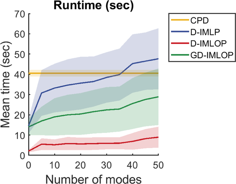
Leave-one-out experiment: mean time taken by our algorithms to compute registrations using different number of modes.

Fig. 8.

Leave-one-out experiment: residual errors compared against tRE produced by D-IMLP (top-left), D-IMLOP (top-right), and GD-IMLOP (bottom-left), and error produced by CPD compared against the tSE (bottom-right) in Exp. 1. The two measures show correlation using D-IMLP, D-IMLOP and GD-IMLOP with coefficients 0.91, 0.65 and 0.61, respectively, but not using CPD (correlation coefficient = 0.05).

4.1.2. Experiment 2: Right nasal airway

Since both turbinates would generally not be visible at the same time during an endoscopic procedure, we used the right nasal airway models to generate sample points in this experiment. The left-out right nasal cavity meshes recovered using our algorithms were again comparable to the estimates produced by the SSM, with GD-IMLOP producing mean tSE errors almost equal to those produced by the SSM up to about 30 modes (Fig. 9, top). Of the 1749 runs, 61.01% of the D-IMLP runs recovered the left out mesh with mean tRE less than 1 mm compared to 86.16% and 98.51% of D-IMLOP and GD-IMLOP runs, respectively. The mean tREs produced by D-IMLP, D-IMLOP, and GD-IMLOP over all runs were 1.15 (± 0.63) mm,0.76 (± 0.40) mm (p < 0.001 compared to D-IMLP), and 0.60 (± 0.16) mm (p < 0.001 compared to both D-IMLP and D-IMLOP), respectively. As in the previous experiment, the performance of D-IMLP deteriorated quickly as the number of shape parameters increased. With added orientation, D-IMLOP either maintained performance or deteriorated slowly with increasing number of shape parameters, while GD-IMLOP either showed improvement or was able to maintain performance (Fig. 9). As before, these improvements can be attributed to increasing the amount of information available by adding orientations and making appropriate noise assumptions in the presence of increased number of parameters to estimate.

Fig. 9.

Leave-one-out experiment: mean tRE (top-left), tSE (top-right), translation and rotation errors (bottom) obtained using different number of modes to estimate the left-out right nasal cavity meshes and recover the transformations in Exp. 2.

We were not able to compare results from this experiment to CPD because our machine was unable to handle the memory overhead of CPD with larger meshes. CPD computes a n_v × n_v matrix, where n_v is the number of vertices in the deformable mesh. This results in extremely large memory requirements even for medium sized meshes, a drawback that our methods do not suffer from.

4.2. Partial data experiment

This experiment is set up similarly to the leave-one-out experiments, but in order to simulate more realistic scenarios, we used the pelvis and right nasal cavity SSMs to generate point samples from part of the left out shape, rather than uniformly from the entire mesh, for each registration (Fig 10). The part of the meshes that points are generated from depends on the procedure being simulated. We design two experiments simulating two different procedures. For both experiments, 2000 points are sampled from the candidate regions of the meshes with appropriate noise added to the sampled points.

Fig. 10.

An example of data generated for the partial data experiment: (left) points are sampled only from the ilium and ischium on the pelvis mesh, and (right) points are sampled from the front section of the right nostril which include parts of the septum and middle and inferior turbinates.

Although we do not have results from CPD due to computational limitations of CPD with relatively large meshes, we can assume that it would not perform as well in recovering the shape because CPD only deforms the parts of the mesh that sample points are matched to and not the overall mesh.

4.2.1. Experiment 1: Pelvis

Using the pelvis dataset, we simulate a situation in which only a partial CT scan of the pelvis is obtained to prevent radiation exposure to reproductive organs. Points are sampled only from this partial scan containing the ilium and the ischium (Fig 10, left), and anisotropic noise with SDs of 1 × 1 × 2 mm³ and 10° (e = 0.5) is added to position and orientation data, respectively. An instance of the pelvis is estimated by our algorithms using these sampled points and a generous noise assumption with SDs of 2 × 2 × 3 mm³ and 30° (e = 0.5) for position and orientation data, respectively. Our algorithms adjust these noise assumptions based on inlying matches found in each iteration (Billings et al., 2015). Noise assumptions are also restricted from becoming too large in the case of partial data availability to avoid instabilities (Billings et al., 2015).

Results show a big improvement in both transformation parameters and tSE going from 0 to 10 modes (Fig. 11). However, with over 10 modes, the improvement in transformation parameters stabilizes, and only a gradual improvement in tSE is observed, although the trend followed by the tSE is similar to that followed by the error between the left out shape and the SSM instance of the left out shape (Fig. 11, top-right). The resulting tRE falls below 2 mm, the desired accuracy for pelvis registrations, with only 10 modes (Fig. 11, top-left). The mean tREs produced by D-IMLP, D-IMLOP, and GD-IMLOP over all runs were 2.10 (± 0.54) mm, 1.96 (± 0.51) mm (p < 0.001 compared to D-IMLP), and 1.96 (± 0.56) mm (p < 0.001 compared to D-IMLP), respectively. The improvement in these errors is also reflected in the residual errors produced by our algorithms (Fig. 13, left).

Fig. 11.

Partial data experiment: mean tRE (top-left), tSE (top-right), translation and rotation errors (bottom) obtained using different number of modes to estimate the left-out pelvis meshes and recover the transformations in Exp. 1.

Fig. 13.

Partial data experiment: residual errors compared against tRE for GD-IMLOP in (L) Exp. 1 using pelvis data (correlation coefficient = 0.56) and (R) Exp. 2 using right nasal cavity data (correlation coefficient = 0.64).

4.2.2. Experiment 2: Right nasal airway

Using the right nasal cavity models, we simulate points that would be generated from nasal endoscopy. Points are sampled only from parts of the nasal cavity that would be visible to the endoscope when inserted into the nose (Fig 10, right) and anisotropic noise with SDs of 0.5 × 0.5 × 1 mm³ and 10° (e = 0.5) is added to position and orientation data, respectively, since this produced point clouds that resembled reconstructions obtained from in vivo data using the method described in the following section (Sec. 4.3). Positional noise in the generated samples has a larger standard deviation in the z-direction because depth is harder to estimate from video. The left out nasal cavity is then estimated using these sampled points and a noise model assumption with SDs of 1 × 1 × 2 mm³ and 30° (e = 0.5) for position and orientation data, respectively.

This experiment yielded slightly different results due to the increased complexity of this data. Although the rotation errors either remained stable or showed improvement with increasing number of modes, rotation errors remained stable or degraded, as in the case of D-IMLOP (Fig. 12, bottom). The tSE only showed steady improvement in the case of GD-IMLOP (Fig. 12, top-right). However, the mean tSE for all algorithms remained below 1 mm. Combined, only GD-IMLOP showed improved tREs as the number of modes increased and consistently produced errors below 1 mm (Fig. 12, top-left). Mean tREs produced by D-IMLP, D-IMLOP, and GD-IMLOP over all runs were 1.29 (± 0.31) mm, 1.00 (± 0.25) mm (p < 0.001 compared to D-IMLP), and 0.80 (± 0.18) mm (p < 0.001 compared to both D-IMLP and D-IMLOP), respectively. Improvement in errors produced by GD-IMLOP is reflected in the residual errors produced by the algorithm (Fig. 13, right).

Fig. 12.

Partial data experiment: mean tRE (top-left), tSE (top-right), translation and rotation errors (bottom) obtained using different number of modes to estimate the left-out right nasal cavity meshes and recover the transformation in Exp. 2.

4.3. Clinical data experiment

An anonymized in vivo clinical dataset consisting of endoscopic video of the nasal cavity and EM-tracking information was obtained from several patients who were examined at the Johns Hopkins Outpatient Center. Permission to collect this dataset, given patient consent, was approved by the Johns Hopkins internal review board (IRB) under application number NA 00074677.

A modified version of the learning-based photometric reconstruction technique developed by Reiter et al. (2016) was used to reconstruct structures from endoscopic video collected from patients who volunteered to enroll in our study. Structure from motion (SfM) points obtained from video sequences (Leonard et al., 2016, 2018) were used to train a self-supervised deep neural network that enforces depth consistency between frames using relative pose information from SfM (Liu et al., 2018). This network was then used to predict the depth associated with each pixel in a single video frame. This method computes highly dense reconstructions of structures visible in the frame. 2000 points each were sampled from reconstructions from two different frames. These samples were manually initialized in the mean left nasal cavity mesh, and registered using our algorithms with 10 modes restricted within ±1 SD. The scale estimation was restricted within [0.7, 1.3], and anisotropic noise models with SDs of 1 × 1 × 2 mm³ and 40° (e = 0.5) were assumed for position and orientation, respectively.

For the first set, D-IMLP failed to produce a meaningful registration due to lack of sufficient information since it does not use orientation information (Fig 14, top-left), and D-IMLOP failed due to incorrect angular noise assumptions (Fig 14, top-middle). GD-IMLOP, however, was able to produce submillimeter residual error of 0.92 (±1.44) mm (Fig 14, top-right). We also compute the tSE between shapes computed by our algorithms and the patient shape automatically segmented as described before in Sec. 2. GD-IMLOP was able to estimate the patient shape with a mean tSE of 0.98 (±0.8) mm.

Fig. 14.

Clinical data experiment: With the first point set (top), registration results using D-IMLP (left) and D-IMLOP (middle) show failed registrations, while that using GD-IMLOP (right) shows good alignment (along with some outliers). The second point set (bottom) yields better results, with all three algorithms producing good alignments. However, we can see that the number of outliers or bad matches (red points matched to the outside of the nose) goes down as we go from D-IMLP (left) to D-IMLOP (middle) to GD-IMLOP (right).

Using the second set of samples, GD-IMLOP converged with a residual error of 0.77(±1.18) mm (Fig 14, bottom-right), and D-IMLOP and D-IMLP also produced submillimeter residual errors of 0.6 (±0.98) mm and 0.5 (±0.82) mm, respectively (Fig 14, bottom-left and bottom-middle). All three algorithms also recover the patient shape successfully with tSEs of 0.95 (±0.88) mm, 0.95 (±0.83) mm, and 0.96 (±0.83) mm for GD-IMLOP, D-IMLOP, and D-IMLP, respectively.

5. Discussion

In summary, our experiments show that our algorithms exhibit improved performance with increasing number of modes, and GD-IMLOP outperforms both D-IMLOP and D-IMLP. This is expected since GD-IMLOP is the most generalized of the algorithms presented and, therefore, is able to best model the noise in the data used for our experiments. The leave-out analysis shows that GD-IMLOP can match the SSM instance of the left-out shape for some number of modes. However, GD-IMLOP is slower than D-IMLOP since it solves a more complex objective function. This trade-off between runtime and accuracy is important to keep in mind for difference applications. GD-IMLOP was able to maintain performance in increasingly difficult setting such as partial data and unknown noise. Finally, our clinical evaluations also result in submillimeter mean residual errors and tSEs.

6. Conclusions and future work

In this paper, we have presented a deformable registration paradigm that can be used to build several different types of registration algorithms that simultaneously solve for both transformation and shape parameters. We demonstrate this with three algorithms that use different types of features and noise models. Additional algorithms can be developed under this paradigm using different or additional features (e.g., occluding contours or non-geometric features like RGB values associated with points), assuming different noise models that better explain certain types of data (e.g., Poisson distribution), or utilizing different types of generative SSMs (e.g., those that do not assume Gaussian distribution in the data or that the data lie in a single subspace).

Our algorithms are validated through several different experiments that show that our methods, especially those that use orientation information in addition to position, can estimate transformation and shape parameters with high accuracy. This result is further strengthened by the promising performance of our algorithms in preliminary experiments with in vivo nasal endoscopy data. Our algorithms also provide an added advantage in that the error metrics produced by them correlate with tRE, allowing our algorithms to assign confidence to the registrations produced based on the residual errors produced by them.

In the future, we hope to build more extensive shape models of anatomy using many more CT images (on the order of thousands) to better explain the variation in different anatomical structures, and also to conduct more clinical experiments with reconstructions from multiple video frames and spanning a larger extent of the nasal passage. This will allow us to better establish how well we are able to infer anatomical structures that we do not see in video or have samples from. We also hope to explore other statistical shape models that can better explain the variation in more complex regions of the sinuses like the ethmoid cells which have a honeycomb-like structure. Additionally, we plan to incorporate more features, like occluding contours (Billings et al., 2016), into our framework to further strengthen the application of these methods in the medical field.

SSMs can also be used in applications outside the medical field. Initial exploration in learning the range of human facial expression has shown promising results (Sec. Appendix A.5). While facial expressions may be hard to visualize when represented as point clouds, we expect that with enough shapes and the right SSM, we can infer emotion by registering a statistically derived shape to the point cloud and reconstructing the expression being rendered. We also hope to build models better suited to explain complex data like pose variation, and incorporate these models, in addition to PCA models, into our framework to enable tasks like pose classification. Our code is available at https://github.com/AyushiSinha/cisstICP.

Highlights.

• Presenting a novel deformable registration paradigm using statistical shape models

• Developed three algorithms that use different features and noise model assumptions

• Experiments with simulated data show submillimeter registrations, reconstructions

• Preliminary results on in-vivo clinical data also show promising results

Appendix A. Additional experiments and results

We performed several additional experiments to study our algorithms. Results from these experiments are presented here.

Appendix A.1. Sample size experiment

For this experiment, we generated a synthetic dataset using the mean shape and SSM from the pelvis dataset. We deformed the mean pelvis shape by known shape parameters sampled within ±3 SD, sampled oriented points from the deformed shapes, and then applied known transformations within realistic intervals to the sampled points. Experiments were run with 500, 1000, 1500 and 2000 sample points to evaluate the performance of our algorithms with increasing number of samples.

For each algorithm, 3 sets of experiments were run with 0, 5, and 10 modes used to deform the mean shape. In this experiment, the same number of modes are used by our algorithms to estimate the deformed shape as were used to deform the mean shape in order to evaluate our algorithms’ performance with different modes without bias. As before, when 0 modes are used, the algorithms used are the corresponding non-deformable algorithms performing rigid registration between the mean shape and points sampled from it. 10 registrations were performed in each set with known transformations sampled from the intervals [0, 15] mm and [0, 9]° for translational and rotational offsets, respectively, and applied to points sampled from the deformed shapes. Noise was added to both the position and orientation of the sampled points, and two experiments were designed based on different noise models.

Appendix A.1.1. Experiment 1: Isotropic position noise

In this experiment, an isotropic noise model with SD of 1 × 1 × 1 mm³ for positional noise was used to generate samples. Additionally, an isotropic noise model with SD of 2° for angular noise was used for D-IMLOP. For GD-IMLOP, the anisotropic angular noise model also had a SD of 2° and e was set to 0.5. The noise model assumed by each of the algorithms was the same as the noise model used to generate samples for each of the algorithms.

All three of our algorithms produced small errors in recovering the shape and registering the sampled points to the recovered shape with the different number of samples. D-IMLOP and GD-IMLOP outperformed D-IMLP due to the added information provided by the normals (Fig. A.15). Over all runs, D-IMLP produced a mean tRE of 0.71 (± 0.80) mm, while D-IMLOP and GD-IMLOP produced mean tREs of 0.30 (± 0.32) mm (p < 0.001 compared to D-IMLP) and 0.29 (± 0.35) mm (p < 0.001 compared to D-IMLP), respectively. D-IMLOP slightly outperformed GD-IMLOP in recovering rotation. This is because D-IMLOP solves a relatively simpler objective function since it only models isotropic orientation noise. Since the orientation noise in the samples used for D-IMLOP is also isotropic, the algorithm is able to converge toward the correct rotation quickly. For GD-IMLOP, however, the objective function is more complicated since it models anisotropic orientation noise making GD-IMLOP slower to converge to the correct rotation in some cases.

Further, metrics produced by our algorithms, like the objective function (total match error) or the residual error (Mahalanobis distance), show correlation with the tRE and can be used to assign confidence to the computed registration. We used empirically chosen thresholds to determine which trials succeeded and which did not using the residual error. We do this retrospectively in the simulated experiments because we have access to ground truth and can use it to learn how to associate residuals errors with success in clinical or other experiments where ground truth in not available. Using thresholds such that there were no false positives, our algorithms were always able to correctly detect successful registrations and showed an increase in successful registrations with increasing number of sample points (Fig. A.15, Table A.1), where success is defined as registrations producing tRE less than 1.5 mm for the pelvis dataset. In fact, all D-IMLOP and GD-IMLOP trials using greater than 500 sample points produced successful registrations.

Appendix A.1.2. Experiment 2: Anisotropic position noise

Second, an anisotropic noise model with 1 mm SD in each direction in plane and 2 mm out of plane was used for positional noise (or, 1 × 1 × 2 mm³). For angular noise, the parameters were the same as in Exp. 1.

The tREs from this experiment were higher than those in Exp. 1 but by less an 0.1 mm for all algorithms. Most D-IMLP trials and all D-IMLOP and GD-IMLOP trials produced successful registrations (Table A.1). D-IMLOP performs slightly better than GD-IMLOP in recovering rotation due to the same reason as in Exp. 1 (Fig. A.16). However, GD-IMLOP is able to achieve smaller tREs than D-IMLOP since it outperforms D-IMLOP in recovering translation and shape parameters (Fig. A.17). Again, over all runs, D-IMLP produced a mean tRE of 0.76 (± 0.75) mm, while D-IMLOP and GD-IMLOP produced mean tREs of 0.39 (± 0.33) mm (p < 0.001 compared to D-IMLP) and 0.33 (± 0.28) mm (p < 0.001 compared to D-IMLP), respectively. An improvement with increasing number of sample points was observed in this experiment as well (Fig. A.17). Note that errors show some increase with increasing number of modes because, as mentioned in the experiment setup, number of modes used by our algorithms to estimate the deformed target shape was the same as the number of modes used to generate the target shape. The residual errors from all three algorithms were, again, found to be correlated with the tRE (Fig. A.19) and, therefore, can be used to assign confidence to registrations. Using empirically found thresholds, we used the residual errors produced by our algorithms to automatically classify trials as successful or unsuccessful and again found that our algorithms were always able to correctly classify successful registrations (Table A.1).

Since D-IMLOP and GD-IMLOP are able to filter out matches where positions align but orientations do not, we see faster improvement in the quality of matched points with these two algorithms than with D-IMLP. (Fig. A.18). Here, the error shown is the distance at each iteration between the matched points computed by each algorithm and the true location of the matched point. This true location is simply the location of the points sampled from the deformed model shape before any noise or transformation was applied. This illustrates the improvement afforded by orientation information.

Appendix A.2. Noise model experiment

This experiment was designed to evaluate the stability of our algorithms with different noise models. A synthetic dataset was generated using the pelvis data in a similar way as described in Sec. Appendix A.1. The differences are that experiments in this section are run with a fixed sample size of 500, and for each algorithm, 11 sets of 25 experiments each are run with increasing number of modes used to deform the mean shape in each set, starting at 0 and going up to 10 modes. Again, the same number of modes are used by our algorithms to recover the deformed shape as were used to generate the deformed shape. Different noise models were used to add noise to both the position and orientation of the sampled points, and the same noise models were assumed by our algorithms. Four experiments were designed based on how the different noise models were varied.

Appendix A.2.1. Experiment 1: Varying isotropic position noise

For the first experiment, we used 5 isotropic noise models with SDs of 1 × 1 × 1 mm³, 2 × 2 × 2 mm³, 3 × 3 × 3 mm³, 4 × 4 × 4 mm³, and 5 × 5 × 5 mm³ for positional noise. For D-IMLOP, an isotropic noise model with SD of 2° for angular noise was used, while an anisotropic noise model with SD of 2° and e = 0.5 was used for GD-IMLOP.

We observed that registrations produced by our algorithms degraded as the noise in the sample points increased, but tREs also showed improvement going from D-IMLP to D-IMLOP to GD-IMLOP (Fig. A.20, top row). Over all registrations, D-IMLP produced a mean tRE of 1.55 (± 0.96) mm, while D-IMLOP and GD-IMLOP produced mean tREs of 0.75 (± 0.60) mm (p < 0.001 compared to D-IMLP) and 0.40 (± 0.22) mm (p < 0.001 compared to both D-IMLP and D-IMLOP), respectively. Further, while noise increased 125× (5× along each dimension), tREs only degraded 1.78× at 1 mode and 2.18× at 10 modes for D-IMLP, 1.48× at 1 mode and 2.33× at 10 modes for D-IMLOP, and 1.44× at 1 mode and 1.26× at 10 modes for GD-IMLOP. By compensating for the noise in the samples, our algorithms are able to limit the effects of increasing noise on the registration.

The tREs increase slightly as we add more modes because, as described in the experiment setup, the number of modes used by our algorithms to estimate the deformed target shape was the same as the number of modes used to generate the deformed target shape. That is, for 0 modes, points were sampled from the mean shape without any deformation and no shape parameters were used in the optimization, resulting in the rigid versions of our algorithms. Whereas when 10 modes are used, the mean shape is deformed along 10 mode directions and 16 parameters are optimized by our algorithms (10 shape parameters as well as 3 rotation and 3 translation parameters). The objective function and the residual errors are again found to be strongly correlated with the tRE, which again can be used to distinguish between successful and unsuccessful registrations (Fig. A.21).

Appendix A.2.2. Experiment 2: Varying anisotropic position noise

For the second experiment, anisotropic noise models with SDs of 1×1×2 mm³, 2×2×3 mm³, 3×3×4 mm³, 3×3×5 mm³, and 4 × 4 × 5 mm³ for positional noise were used. For angular noise, the parameters were the same as in Exp. 1.

Results from this experiment show the same trends as those from Exp. Appendix A.2.1 (Fig. A.20, middle row). Over all runs, D-IMLP produced a mean tRE of 1.97 (± 1.06) mm, while D-IMLOP and GD-IMLOP produced mean tREs of 0.80 (± 0.56) mm (p < 0.001 compared to D-IMLP) and 0.38 (± 0.20) mm (p < 0.001 compared to both D-IMLP and D-IMLOP), respectively. Additionally, while noise increased 40× (4× along each dimension in plane and 2.5× out of plane), the tREs only degraded 1.08× at 1 mode and 1.29× at 10 modes for D-IMLP, 1.54× at 1 mode and 1.78× at 10 modes for D-IMLOP, and 1.12× at 1 mode and 1.21× at 10 modes for GD-IMLOP.

Appendix A.2.3. Experiment 3: Varying orientation noise

In the third experiment, we used one isotropic noise model and one anisotropic noise model with SDs of 1 × 1 × 1 mm³ and 1 × 1 × 2 mm³, respectively, for positional noise, and used orientation noise models with SDs of 2°, 4°, 6°, 8° and 10° for each positional noise model. e = 0.5 was used for GD-IMLOP.

We observe that all D-IMLP runs with isotropic positional noise produce similar results and all runs with anisotropic positional noise also produce similar results. This is expected since D-IMLP does not take any orientation information into consideration, so varying the orientation noise model has no statistically significant effect on results from D-IMLP. Further, as seen in the previous two experiments, mean tREs from trials with isotropic positional noise (1.04 ± 0.85 mm) are statistically significantly lower (p < 0.001) than those from trials with anisotropic noise (1.74 ± 1.14 mm) (Fig. A.20, bottom-left). The difference in tREs between runs with isotropic and anisotropic positional noise was smaller for D-IMLOP (0.53 ± 0.42 mm and 0.61 ± 0.42 mm, respectively) and GD-IMLOP (0.51 0.42 mm and 0.58 ± 0.46 mm, respectively), although still statistically significant (p < 0.001). As with D-IMLP, changing angular noise did not affect registration results from D-IMLOP and GD-IMLOP statistically significantly since the large number of samples overwhelmed the relatively small changes in the noise model (Fig. A.20, bottom-middle and bottom-right).

Appendix A.2.4. Experiment 4: Noise parameter sweep

In the final experiment, the sample points are generated with a particular noise model for both position and orientation data. However, we assume that this noise model is unknown to our algorithms. Sample points are generated with anisotropic positional and angular noise with SD 2 × 2 × 4 mm³ and 10° (e = 0.5), respectively. We perform a hyper-parameter sweep and run our algorithms with different isotropic and anisotropic positional and angular noise assumptions to see how well our algorithms perform with inaccurate noise model assumptions.

This experiment was performed to observe the behavior of our algorithms when the noise model assumed is different from the noise in the sampled points. Since the noise in the generated sampled points, anisotropic in both position and orientation (2 × 2 × 4 mm³ and 10° (e = 0.5), respectively), can be best explained by GD-IMLOP, we expect it to outperform the other two algorithms. Interestingly, D-IMLOP (red) outperforms GD-IMLOP (green) with less conservative noise estimates (Fig. A.23). This is expected since D-IMLOP optimizes a simpler cost function. Therefore, when the noise assumption is optimistic, D-IMLOP converges faster than GD-IMLOP. However, as the noise assumption becomes more conservative, GD-IMLOP’s performance improves or stabilizes while D-IMLOP’s deteriorates since GD-IMLOP models the noise in the sample points more accurately. Here, the tRE values are less important than the trends shown by D-IMLOP and GD-IMLOP. D-IMLOP performs well with less conservative noise models since the noise in the samples is close enough to the least conservative noise model assumed by D-IMLOP. However, with larger sample noise, less conservative noise estimates will introduce errors in matches. The improving trend with increasingly conservative noise estimates exhibited by GD-IMLOP allows us to make very conservative noise estimates when sample noise is unknown and still expect reasonable registration results.

Finally, we see that D-IMLP (blue) is unaffected by changing orientation noise, which is expected since D-IMLP does not take orientation into account. tREs using D-IMLP are either stable or show a gradual trend downward as position noise becomes more conservative. The other noticeable trend shows that D-IMLP performs slightly worse as the anisotropy in the noise estimates increases. This trend is slightly visible in the curves for D-IMLOP and GD-IMLOP as well, although they are not as noticeable since the orientation information available to these algorithms is able to drive the errors down considerably.

Appendix A.3. Outlier experiment

Using a synthetic dataset generated using the right nasal cavity model from the sinus dataset, we study how robust our algorithms are to outliers. This dataset was again generated similarly as described before (Sec. Appendix A.1); the difference being that in this setup, there are 6 sets of 10 experiments each for all three algorithms. The number of modes used to deform the mean shape increases by 2 in each set, starting at 0 and going up to 10 modes. Again, the same number of modes are used to estimate the deformed target shape using our algorithms as were used to generate the deformed target shape.

All sample points were generated with isotropic noise in position data with 1 × 1 × 1 mm³ SD, and anisotropic noise in orientation data with 2° SD and e = 0.5. Experiments were conducted with 0%, 10%, and 20% outliers in the generated point samples. Outliers are generated by perturbing the position and orientation of a particular number of samples randomly in the range [2, 5] mm and [2, 5]°, respectively.

Outliers are identified and rejected using the chi-square test, in the same way as in the corresponding rigid algorithms described earlier (Billings et al., 2015; Billings and Taylor, 2015). Under the assumption of correspondences and generalized Gaussian noise, the square Mahalanobis distance between the matched points in 3D space can be assumed to distributed as the sum of squares of three independent Gaussian distributions, each representing one dimension of position data (Danilchenko and Fitzpatrick, 2011). Therefore, a match is rejected if the square Mahalanobis distance is greater than the chi-square inverse cumulative density function with 3 degrees of freedom at p = 0.95. For orientation data, a match that passes the outlier test based on the position component can still be rejected if ${\widehat{\mathbf{y}}}_{{\mathbf{n}}_i}^{\mathbf{T}}{\widehat{\mathbf{x}}}_{{\mathbf{n}}_i}<\cos \hspace{0.17em}({\theta }_{\text{thresh}})$, where θ_thresh is set according to the circular SD. We set our threshold to 3 times the circular SD.

Although the performance of our algorithms is worse in the presence of outliers, we are able to detect them, as explained above (Sec. Appendix A.3), and limit their effect on errors. The degradation in performance as outliers increase 2× from 10% to 20% is, at worst, 1.45× (using 4 modes), 1.72× (using 2 modes) and 1.42× (using 4 modes) for D-IMLP, D-IMLOP and GD-IMLOP, respectively. At best, the performance is almost identical for all algorithms: 1.12×, 0.97× and 1.10× for D-IMLP, D-IMLOP and GD-IMLOP, respectively, all using 10 modes (Fig. A.22). As outliers increase from 0% to 20%, the degradation in performance is, at worst, 2.81×, 2.18× and 2.53× for D-IMLP, D-IMLOP and GD-IMLOP, respectively, all using 4 modes. At best, the performance degrades 1.79× (using 6 modes), 1.21× (using 8 modes) and 1.93× (using 6 modes) for D-IMLP, D-IMLOP and GD-IMLOP, respectively. However, we cannot compare this to the degradation in the quality of samples points since the initial set had 0% outliers (making any increase an ∞ increase).

Although the addition of outliers produced statistically significant increases in tREs for D-IMLP and GD-IMLOP, the increase in tREs from 0% to 10% outliers and from 10% to 20% outliers was not statistically significant for D-IMLOP. However, the increase in tREs from 0% to 20% outliers was statistically significant for D-IMLOP as well (Table A.2). Further, Fig. A.22 (bottom-right) shows that without any outliers in the sampled point set, GD-IMLOP performs best, followed by D-IMLOP, and then D-IMLP (as seen in previous experiments). Fig. A.22 (bottom-right) also shows a very strong result in that although with 10 modes, GD-IMLOP must optimize over 10 extra parameters, the degradation in the tRE is negligible (~ 0.05 mm) with 0% outliers (green).

Appendix A.4. Scale experiment

In this experiment, we evaluate how well our algorithm is able to recover scale in addition to rotation, translation, and shape parameters. We use the same dataset that was generated in Sec. Appendix A.3 with 0% outliers. However, the sample points are scaled by some known amount in the range [0.7, 1.3].

Results show that our methods can successfully estimate scale in addition to rotation, translation, and shape parameters. Although our methods perform better when there is one fewer parameter to optimize over (Table A.3), with an additional scale parameter, tSEs using all three algorithms and tREs using D-IMLOP and GD-IMLOP still remain consistently below 1 mm (Fig. A.25, left and middle). Errors in recovering scale also reflect D-IMLOP and GD-IMLOP’s performance, with mean errors ~ 0.01 and SD < 0.01 (Fig. A.25, right).

Appendix A.5. Non-medical data experiment

Our previous experiments test the generalizability of our algorithms within the medical field. With the following experiment, we test our algorithms on non-medical data to test their generalizability outside the medical field. We use a human expression dataset in a leave-n-out experiment by dividing the dataset into a training set and a test set. We use the training set to build a shape model, and estimate the meshes in the test set using the two methods described in Sec. 4.1.

We used 300 meshes in the training set to build an SSM for expressions from a single individual, and tested with the remaining 86 meshes in the test set, also from the same individual. 1000 points were sampled from meshes in the test set with anisotropic position and orientation noise with SDs 1 × 1 × 2 mm³ and 10° (e = 0.5), respectively. This simulates a realistic situation in which a scan of a head is obtained using a depth camera, where error is large in the depth direction. Our algorithms make slightly more relaxed noise assumptions, assuming that the position and orientation noise models to have SDs of 2 × 2 × 4 mm³ and 20° (e = 0.5), respectively.

Results from this experiment show that our algorithms perform relatively well even with challenging datasets. The assumption that facial expressions are Gaussian distributed is likely an incorrect assumption depending on the dataset (Buciu et al., 2008). Further, the limited number of data points in our dataset was not enough to explain well the complex variations that can exist in human expression. However, our algorithms produced promising results with tSEs and tREs consistently below 1 mm and 2 mm, respectively (Fig. A.24). Over all runs, D-IMLP produced a mean tRE of 1.78 (± 0.63) mm, D-IMLOP produced mean tRE of 1.66 (± 0.60) mm (p < 0.001 compared to D-IMLP) and and GD-IMLOP produced mean tRE of 1.38 (± 0.48) mm (p < 0.001 compared to both D-IMLP and D-IMLOP), respectively. With more data and more sample points, we can likely perform well enough with our PCA model to attempt to classify the facial expressions (Fig. A.26). The residual errors produced by our algorithms also correlate with the tRE, indicating that our algorithms have the ability to handle such data (Fig. A.27).

Fig. A.15.

Sample size experiment: translation (top) and rotation (bottom) errors produced using (from L to R) 1000 and 2000 sample points from the pelvis model in Exp. 1. Bars in the histogram are transparent to show all three algorithms.

Fig. A.16.

Sample size experiment: translation (top) and rotation (bottom) errors produced using (from L to R) 1000 and 2000 sample points from the pelvis model in Exp. 2. Bars in the histogram are transparent to show all three algorithms.

Fig. A.17.

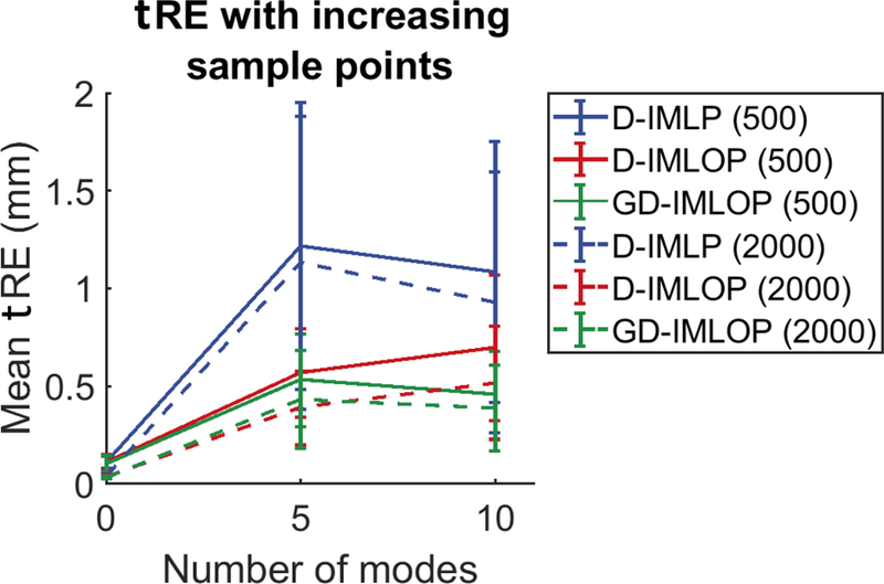
Sample size experiment: mean tRE with increasing number of samples from Exp. 2 (shown with 500 and 2000 sample points for simplicity).

Fig. A.18.

Sample size experiment: evolution of the quality of matched points for each algorithm with increasing iterations in Exp. 2 with 2000 sample points. The plot shows distances between matched points at each iteration and the location of points sampled from the deformed model shape. Added orientations drastically improve the quality of matched points.

Fig. A.19.

Residual errors compared against tRE using 2000 sample points in Exp. 2 of the sample size experiment. The two measures exhibit correlation with correlation coefficients (left to right) of 0.85, 0.72 and 0.86. Results from trials using 0 modes are ignored here to focus on the deformable algorithms.

Fig. A.20.

Noise model experiment: mean tREs produced by our algorithms (L-R) D-IMLP, D-IMLOP and GD-IMLOP in Exps. 1 (top), 2 (middle) and 3 (bottom). Note that the errors are increasing with increasing modes only because for this experiment the number of modes used to estimate the shapes equals the number of modes used to simulate a new shape from which points were sampled.

Fig. A.21.

Residual errors compared against tRE using 500 sample points with 2 × 2 × 2 mm³ SD positional noise and 2° SD angular noise in Exp. 1 of the noise model experiment. The two measures exhibit correlation with correlation coefficients (L-R) of 0.86, 0.88 and 0.83.

Fig. A.22.

Outlier experiment: mean tRE with different number of outliers for D-IMLP (top-left), D-IMLOP (top-right), and GD-IMLOP (bottom-left), and for all three algorithms using sample points with 0% outliers (bottom-right). Note that the errors are increasing with increasing modes only because for this experiment the number of modes used to estimate the shapes equals the number of modes used to simulate the deformed shape from which points were sampled.

Fig. A.23.

Noise model experiment: mean tREs produced by our algorithms with different isotropic (left) and anisotropic (right) position noise assumptions, labeled on the x-axis, and different orientation noise assumptions, with standard deviations of 2° (top), 10° (middle) and 20° (bottom) in Exp. 4.

Fig. A.24.

Non-medical data experiment: mean tRE (left) and tSE (right) obtained using different number of modes to estimate the test shape using facial expression data.

Fig. A.25.

Scale experiment: Mean tSE (left) and tRE (middle) using sample points with 0% outliers and scale applied to the sampled points, and mean errors in recovering scale with increasing number of modes (right). Again, the number of modes used to estimate the shapes equals the number of modes used to simulate the deformed shape from which points were sampled.

Fig. A.26.

Non-medical data experiment: this particular target shape (right) has a lot of detail which is necessary to convey the emotion in this face. 1000 sample points are too few to capture this detail resulting in an inaccurate reconstruction (left). However, with 2000 sample points, we are able to estimate this expression better (middle) since more sample points are better able to capture the detail in the target.

Fig. A.27.

Non-medical data exp.: residual errors compared against tRE for GD-IMLOP using facial expression data. The two measures show correlation (correlation coefficient = 0.77).

Table A.1.

Sample size experiment: percent successful trials, i.e., trials producing registrations with tRE less than 1.5 mm. All successful trials were correctly detected as successful.

	samples	Algorithm (success in %)
		D-IMLP	D-IMLOP	GD-IMLOP
Exp. 1	500	83.33	96.67	96.67
	1000	86.67	100.00	100.00
	1500	83.33	100.00	100.00
	2000	86.67	100.00	100.00
Exp. 2	500	76.67	100.00	100.00
	1000	76.67	100.00	100.00
	1500	76.67	100.00	100.00
	2000	76.67	100.00	100.00

Table A.2.

Outlier experiment: mean tREs produced by each of our algorithms with 0%, 10%, and 20% outliers in the samples points.

outliers	Algorithm (tREs in mm)
	D-IMLP	D-IMLOP	GD-IMLOP
0%	0.37 ± 0.25	0.19 ± 0.15	0.08 ± 0.03
10%	0.58 ± 0.36*	0.26 ± 0.23	0.14 ± 0.05*
20%	0.75 ± 0.30†	0.30 ± 0.18‡	0.18 ± 0.05†

^*indicates statistically significant increase in tREs between 0% and 10% outliers

^†indicates statistically significant increase in tREs between both 10% and 20% outliers and 0% and 20% outliers

^‡indicates statistically significant increase in tREs between 0% and 20% outliers (p < 0.001).

Table A.3.

Scale experiment: mean tREs produced by each of our algorithms with and without scale.

	Algorithm (tREs in mm)
	D-IMLP	D-IMLOP	GD-IMLOP
w/o scale	0.37 ± 0.25	0.19 ± 0.15	0.08 ± 0.03
w scale	1.11 ± 0.45*	0.68 ± 0.34*	0.10 ± 0.03*

^*indicates statistically significant (p < 0.001) increase in tREs when optimizing over an additional scale parameter.

References

- Amberg B, Romdhani S, Vetter T, 2007. Optimal step nonrigid icp algorithms for surface registration, in: 2007 IEEE Conference on Computer Vision and Pattern Recognition, pp. 1–8. doi: 10.1109/CVPR.2007.383165. [DOI] [Google Scholar]
- Avants BB, Tustison NJ, Song G, Cook PA, Klein A, Gee JC, 2011. A reproducible evaluation of ants similarity metric performance in brain image registration. NeuroImage 54, 2033–2044. doi: 10.1016/j.neuroimage.2010.09.025. [DOI] [PMC free article] [PubMed] [Google Scholar]
- Avants BB, Yushkevich P, Pluta J, Minkoff D, Korczykowski M, Detre J, Gee JC, 2010. The optimal template effect in hippocampus studies of diseased populations. NeuroImage 49, 2457–2466. doi: 10.1016/j.neuroimage.2009.09.062. [DOI] [PMC free article] [PubMed] [Google Scholar]
- Beichel RR, Ulrich EJ, Bauer C, Wahle A, Brown B, Chang T, Plichta KA, Smith BJ, Sunderland JJ, Braun T, Fedorov A, Clunie D, Onken M, Riesmeier J, Pieper S, Kikinis R, Graham MM, Casavant TL, Sonka M, Buatti JM, 2015. Data from qin-headneck. The Cancer Imaging Archive doi: 10.7937/K9/TCIA.2015.K0F5CGLI. [DOI] [Google Scholar]
- Berger G, Eviatar E, Kogan T, Landsberg R, 2013. The normal uncinated process: histology and clinical relevance. European Archives of Oto-Rhino-Laryngology 270, 959–964. doi: 10.1007/s00405-012-2169-2. [DOI] [PubMed] [Google Scholar]
- Besl PJ, McKay ND, 1992. A method for registration of 3-d shapes. IEEE Transactions on Pattern Analysis and Machine Intelligence 14, 239–256. doi: 10.1109/34.121791. [DOI] [Google Scholar]
- Billings SD, 2015. Probabilistic Feature-Based Registration for Interventional Medicine Ph.D. thesis. The Johns Hopkins University. Baltimore, Maryland. [Google Scholar]
- Billings SD, Boctor EM, Taylor RH, 2015. Iterative most-likely point registration (imlp): A robust algorithm for computing optimal shape alignment. PLOS ONE 10, 1–45. doi: 10.1371/journal.pone.0117688. [DOI] [PMC free article] [PubMed] [Google Scholar]
- Billings SD, Sinha A, Reiter A, Leonard S, Ishii M, Hager GD, Taylor RH, 2016. Anatomically Constrained Video-CT Registration via the V-IMLOP Algorithm Springer International Publishing, Cham; pp. 133–141. doi: 10.1007/978-3-319-46726-9_16. [DOI] [PMC free article] [PubMed] [Google Scholar]
- Billings SD, Taylor RH, 2014. Iterative Most Likely Oriented Point Registration Springer International Publishing, Cham. pp. 178–185. doi: 10.1007/978-3-319-10404-1_23. [DOI] [PubMed] [Google Scholar]
- Billings SD, Taylor RH, 2015. Generalized iterative most likely oriented point (g-imlop) registration. International Journal of Computer Assisted Radiology and Surgery 10, 1213–1226. doi: 10.1007/s11548-015-1221-2. [DOI] [PubMed] [Google Scholar]
- Bosch WR, Straube WL, Matthews JW, Purdy JA, 2015. Data from head-neck cetuximab. The Cancer Imaging Archive doi: 10.7937/K9/TCIA.2015.7AKGJUPZ. [DOI] [Google Scholar]
- Bouaziz S, Tagliasacchi A, Pauly M, 2013. Sparse iterative closest point, in: Computer graphics forum, Wiley Online Library; pp. 113–123. [Google Scholar]
- Buciu I, Kotropoulos C, Pitas I, 2008. Comparison of ica approaches for facial expression recognition. Signal, Image and Video Processing 3, 345. doi: 10.1007/s11760-008-0074-3. [DOI] [Google Scholar]
- Chen Y, Medioni G, 1992. Object modelling by registration of multiple range images. Image Vision Comput 10, 145–155. doi: 10.1016/0262-8856(92)90066-C. [DOI] [Google Scholar]
- Chetverikov D, Svirko D, Stepanov D, Krsek P, 2002. The trimmed iterative closest point algorithm, in: Object recognition supported by user interaction for service robots, pp. 545–548 vol.3. doi: 10.1109/ICPR.2002.1047997. [DOI] [Google Scholar]
- Chintalapani G, Ellingsen LM, Sadowsky O, Prince JL, Taylor RH, 2007. Statistical Atlases of Bone Anatomy: Construction, Iterative Improvement and Validation Springer Berlin Heidelberg, Berlin, Heidelberg: pp. 499–506. doi: 10.1007/978-3-540-75757-3_61. [DOI] [PubMed] [Google Scholar]
- Clark K, Vendt B, Smith K, Freymann J, Kirby J, Koppel P, Moore S, Phillips S, Maffitt D, Pringle M, Tarbox L, Prior F, 2013. The cancer imaging archive (tcia): Maintaining and operating a public information repository. Journal of Digital Imaging 26, 1045–1057. doi: 10.1007/s10278-013-9622-7. [DOI] [PMC free article] [PubMed] [Google Scholar]
- Cootes TF, Taylor CJ, Cooper DH, Graham J, 1995. Active shape models—their training and application. Comput. Vis. Image Underst 61, 38–59. doi: 10.1006/cviu.1995.1004. [DOI] [Google Scholar]
- Danilchenko A, Fitzpatrick JM, 2011. General approach to first-order error prediction in rigid point registration. IEEE Transactions on Medical Imaging 30, 679–693. doi: 10.1109/TMI.2010.2091513. [DOI] [PMC free article] [PubMed] [Google Scholar]
- Fedorov A, Clunie D, Ulrich E, Bauer C, Wahle A, Brown B, Onken M, Riesmeier J, Pieper S, Kikinis R, Buatti J, Beichel RR, 2016. Dicom for quantitative imaging biomarker development: a standards based approach to sharing clinical data and structured pet/ct analysis results in head and neck cancer research. PeerJ 4, e2057. doi: 10.7717/peerj.2057. [DOI] [PMC free article] [PubMed] [Google Scholar]
- Ferrante E, Paragios N, 2017. Slice-to-volume medical image registration: A survey. Medical Image Analysis 39, 101–123. doi: 10.1016/j.media.2017.04.010. [DOI] [PubMed] [Google Scholar]
- Granger S, Pennec X, 2002. Multi-scale EM-ICP: A Fast and Robust Approach for Surface Registration Springer Berlin Heidelberg, Berlin, Heidelberg: pp. 418–432. doi: 10.1007/3-540-47979-1_28. [DOI] [Google Scholar]
- Granger S, Pennec X, Roche A, 2001. Rigid Point-Surface Registration using Oriented Points and an EM Variant of ICP for Computer Guided Oral Implantology. Technical Report RR-4169. INRIA URL: https://hal.inria.fr/inria-00072453. [Google Scholar]
- Grupp R, Otake Y, Murphy R, Parvizi J, Armand M, Taylor R, 2016. Pelvis surface estimation from partial ct for computer-aided pelvic osteotomies. Bone Joint J 98, 55–55. [Google Scholar]
- Heimann T, Meinzer HP, 2009. Statistical shape models for 3d medical image segmentation: A review. Medical Image Analysis 13, 543–563. doi: 10.1016/j.media.2009.05.004. [DOI] [PubMed] [Google Scholar]
- Hufnagel H, Pennec X, Ehrhardt J, Ayache N, Handels H, 2009. Computation of a probabilistic statistical shape model in a maximum-a-posteriori framework. Methods Inf Med 48, 314–319. doi: 10.3414/ME9228.314. [DOI] [PubMed] [Google Scholar]
- Kainz J, Stammberger H, 1989. The roof of the anterior ethmoid: A place of least resistance in the skull base. American Journal of Rhinology 3, 191–199. doi:doi: 10.2500/105065889782009552. [DOI] [Google Scholar]
- Koller D, Turitzin M, Levoy M, Tarini M, Croccia G, Cignoni P, Scopigno R, 2004. Protected interactive 3d graphics via remote rendering, in: ACM SIGGRAPH 2004 Papers, ACM, New York, NY, USA: pp. 695–703. doi: 10.1145/1186562.1015782. [DOI] [Google Scholar]
- Leonard S, Reiter A, Sinha A, Ishii M, Taylor RH, Hager GD, 2016. Image-based navigation for functional endoscopic sinus surgery using structure from motion, in: Proc. SPIE, pp. 97840V–97840V–7. doi: 10.1117/12.2217279. [DOI] [PMC free article] [PubMed] [Google Scholar]
- Leonard S, Sinha A, Reiter A, Ishii M, Gallia GL, Taylor RH, Hager GD, 2018. Evaluation and stability analysis of video-based navigation system for functional endoscopic sinus surgery on in vivo clinical data. IEEE Transactions on Medical Imaging 37, 2185–2195. doi: 10.1109/TMI.2018.2833868. [DOI] [PubMed] [Google Scholar]
- Liu X, Sinha A, Unberath M, Ishii M, Hager GD, Taylor RH, Reiter A, 2018. Self-supervised learning for dense depth estimation in monocular endoscopy, in: OR 2.0 Context-Aware Operating Theaters, Computer Assisted Robotic Endoscopy, Clinical Image-Based Procedures, and Skin Image Analysis, Springer International Publishing, Cham; pp. 128–138. doi: 10.1007/978-3-030-01201-4_15. [DOI] [Google Scholar]
- Mardia KV, Jupp PE, 2008. Directional statistics John Wiley & Sons, Inc. Wiley Series in Probability and Statistics, pp. 1–432. doi: 10.1002/9780470316979. [DOI] [Google Scholar]
- Maurer CR, McCrory JJ, Fitzpatrick JM, 1993. Estimation of accuracy in localizing externally attached markers in multimodal volume head images, in: Proc. SPIE doi: 10.1117/12.154535. [DOI] [Google Scholar]
- Myronenko A, Song X, 2010. Point set registration: Coherent point drift. IEEE Transactions on Pattern Analysis and Machine Intelligence 32, 2262– 2275. doi: 10.1109/TPAMI.2010.46. [DOI] [PubMed] [Google Scholar]
- Ogilvy-Stuart AL, Shalet SM, 1993. Effect of radiation on the human reproductive system. Environ Health Perspect 101, 109–116. URL: http://www.ncbi.nlm.nih.gov/pmc/articles/PMC1519954/. [DOI] [PMC free article] [PubMed] [Google Scholar]
- Phillips JM, Liu R, Tomasi C, 2007. Outlier robust icp for minimizing fractional rmsd, in: Sixth International Conference on 3-D Digital Imaging and Modeling (3DIM 2007), pp. 427–434. doi: 10.1109/3DIM.2007.39. [DOI] [Google Scholar]
- Pulli K, 1999. Multiview registration for large data sets, in: Second International Conference on 3-D Digital Imaging and Modeling (Cat. No.PR00062), pp. 160–168. doi: 10.1109/IM.1999.805346. [DOI] [Google Scholar]
- Rangarajan A, Chui H, Mjolsness E, Pappu S, Davachi L, Goldman-Rakic P, Duncan J, 1997. A robust point-matching algorithm for autoradiograph alignment. Medical Image Analysis 1, 379–398. doi: 10.1016/S1361-8415(97)85008-6. [DOI] [PubMed] [Google Scholar]
- Reiter A, Leonard S, Sinha A, Ishii M, Taylor RH, Hager GD, 2016. Endoscopic-ct: learning-based photometric reconstruction for endoscopic sinus surgery, in: Proc. SPIE, pp. 978418–978418–6. doi: 10.1117/12.2216296. [DOI] [PMC free article] [PubMed] [Google Scholar]
- Rusinkiewicz S, Levoy M, 2001. Efficient variants of the icp algorithm, in: Proceedings Third International Conference on 3-D Digital Imaging and Modeling, pp. 145–152. doi: 10.1109/IM.2001.924423. [DOI] [Google Scholar]
- Segal A, Haehnel D, Thrun S, 2009. Generalized-icp, in: Proceedings of Robotics: Science and Systems, Seattle, USA. doi: 10.15607/RSS.2009.V.021. [DOI] [Google Scholar]
- Seshamani S, Chintalapani G, Taylor R, 2011. Iterative Refinement of Point Correspondences for 3D Statistical Shape Models Springer Berlin Heidelberg, Berlin, Heidelberg: pp. 417–425. doi: 10.1007/978-3-642-23629-7_51. [DOI] [PubMed] [Google Scholar]
- Sinha A, Leonard S, Reiter A, Ishii M, Taylor RH, Hager GD, 2016. Automatic segmentation and statistical shape modeling of the paranasal sinuses to estimate natural variations, in: Proc. SPIE, pp. 97840D–97840D–8. doi: 10.1117/12.2217337. [DOI] [PMC free article] [PubMed] [Google Scholar]
- Sinha A, Liu X, Reiter A, Ishii M, Hager GD, Taylor RH, 2018. Endoscopic navigation in the absence of CT imaging, in: MICCAI, Springer Int; pp. 64–71. doi: 10.1007/978-3-030-00937-3_8. [DOI] [Google Scholar]
- Sinha A, Reiter A, Leonard S, Ishii M, Hager GD, Taylor RH, 2017. Simultaneous segmentation and correspondence improvement using statistical modes, in: Proc. SPIE, pp. 101331B–101331B–8. doi: 10.1117/12.2253533. [DOI] [Google Scholar]
- Tao H, Ma Z, Dai P, Jiang L, 1999. Computer-aided three-dimensional reconstruction and measurement of the optic canal and intracanalicular structures. The Laryngoscope 109, 1499–1502. doi: 10.1097/00005537-199909000-00026. [DOI] [PubMed] [Google Scholar]
- Van Kaick O, Zhang H, Hamarneh G, Cohen-Or D, 2011. A survey on shape correspondence, in: Computer Graphics Forum, Wiley Online Library; pp. 1681–1707. [Google Scholar]
- Zhang L, Snavely N, Curless B, Seitz SM, 2004. Spacetime faces: High resolution capture for modeling and animation. ACM Trans. Graph 23, 548–558. doi: 10.1145/1015706.1015759. [DOI] [Google Scholar]
- Zhang Z, 1994. Iterative point matching for registration of free-form curves and surfaces. International Journal of Computer Vision 13, 119–152. doi: 10.1007/BF01427149. [DOI] [Google Scholar]
- Zhu H, Meng F, Cai J, Lu S, 2016. Beyond pixels: A comprehensive survey from bottom-up to semantic image segmentation and cosegmentation. Journal of Visual Communication and Image Representation 34, 12–27. doi: 10.1016/j.jvcir.2015.10.012. [DOI] [Google Scholar]
Associated Data
This section collects any data citations, data availability statements, or supplementary materials included in this article.