A Bayesian approach for individual-level drug benefit-risk assessment

Abstract

In existing benefit-risk assessment (BRA) methods, benefit and risk criteria are usually identified and defined separately based on aggregated clinical data and therefore ignore the individual-level differences as well as the association among the criteria. We proposed a Bayesian multicriteria decision-making method for BRA of drugs using individual-level data. We used a multidimensional latent trait model to account for the heterogeneity of treatment effects with latent variables introducing the dependencies among outcomes. We then applied the stochastic multicriteria acceptability analysis approach for BRA incorporating imprecise and heterogeneous patient preference information.We adopted an efficient Markov chain Monte Carlo algorithm when implementing the proposed method. We applied our method to a case study to illustrate how individual-level benefit-risk profiles could inform decision-making.

1 |. INTRODUCTION

Benefit-risk assessment (BRA) of a drug is a complex but essential activity that pharmaceutical companies, regulators, and health care providers have to perform in multiple stages during the drug’s life cycle.^1,2 With increasing recognition of the importance of this task, board members at regulatory and industry have called for more robust and transparent method-ologies to determine whether the drug’s potential benefits outweigh its risks.^3,4 As a result of this, scientists and clinicians have developed more sophisticated qualitative and quantitative assessments and acknowledged that quantitative BRA plays an important role to complement the qualitative approaches in drug evaluation.⁵

Several recent quantitative approaches have been proposed, among which multicriteria decision analysis (MCDA) was identified to be a promising method to perform a quantitative BRA via providing objectivity and transparency on the impact of weighting and uncertainty.^1,5 The debut of MCDAfor the BRA of new drugs was provided by Mussen et al.⁶ The principle of the method is to compare drugs using utility scores calculated from multiple criteria of benefits and risks, taking into account their relative importance according to the preferences (ie, weights) of the decision-makers. Tervonen et al proposed a stochastic multicriteria acceptability analysis (SMAA) approach that accounts for the uncertainty inherent in both criterion measurements and preference information.⁷ Waddingham et al proposed a Bayesian MCDA model to estimate the distribution of the criterion via synthesizing the evidence observed in previous studies.⁸ van Valkenhoef et al adopted a network meta-analysis to synthesize evidence on the relative effects and safety of a whole network of treatments simultaneously.⁹ Wang et al proposed a stochastic multicriteria discriminatory method that is based on the SMAA and can provide straightforward and informative assistance to decision-making, such as the expected p-values of the evaluation results.¹⁰ Saint-Hilary et al proposed a Dirichlet SMAA, which applied a Dirichlet distribution to the weights of the criteria to unify the MCDA and SMAA.¹¹ Li et al proposed a cumulative meta-analysis plus SMAA framework to incorporate accumulated evidence from clinical trials and update BRA in a longitudinal fashion.¹²

Although these approaches provide valuable insights into drug benefit-risk (BR) evaluation, all of them follow the common practice that constructing separate analyses on efficacy and safety of the drug before integrating the benefits and risks at the population level. These approaches assume uncorrelated benefits and risks and fail to account for heterogeneous responses of patients to the drug. Thus, they may not be appropriate if the patients experiencing harm and the patients experiencing benefit have little overlap. The BR profile concluded on the population level could distort the value of the drug to an individual patient.¹³ Moreover, the patients’ preferences of the different benefits and harms of the drug are heterogeneous within the population and may also differ substantially from that of other key stakeholders. For example, a given safety issue can be tolerated by certain patients but may be unacceptable to others. This perspective aligns with that of the patient-centered care focusing on individual outcomes and to view the patient’s perspective as integral to relevant research.¹³ Therefore, approaches for individual-level BRA are highly desirable.¹⁴

In this article, we propose a personalized multicriteria BRA approach based on SMAA. Specifically, we propose a multidimensional latent trait (MLT) model for efficacy (benefit) and safety (risk) outcomes of treatments, taking into account the effects of covariates on the observed outcomes. Then, we apply a personalized SMAA approach for a specific patient based on his/her preference information and the treatment responses estimated from the MLT. We refer to our proposed framework as MLT-SMAA and use Bayesian approach for model inference and analyses. Bayesian inference, with its coherent approach for integrating different sources of information and uncertainty, along with its link to optimal decision theory, provides a natural framework to perform quantitative BRAs.¹⁵ It also enables the estimation of exact posterior distributions of the parameters based on a smaller samples, while likelihood-based estimation only produces a point estimate of the parameters, with asymptotic standard errors.^16,17

Compared with the current state-of-the-art MCDA approaches, our proposed method have several major difference:(1) Instead of aggregating efficacy and safety outcomes separately to population level first, the MLT-SMAA framework integrates the subject-specific efficacy and safety outcomes before summarizing into a BR composite. Therefore, it could better accommodate scenarios such that different groups of patients experience different level of benefits and risks. (2) MLT-SMAA accounts for the heterogeneity among patients as well as within-patient dependencies among the clinical outcomes (BR criteria) with different data types. This enables more personalized parameter estimates and predictions of the BR trade-offs. (3) MLT-SMAA illustrates a way to incorporate individual-level patient preference information in decision-making, which can help ensure that the BR determinations are patient-centric, resulting in greater use for patients and clinicians.

The rest of this article is organized as follows. In Section 2, we describe a real case study of a clinical trial on a dietary supplement to prevent Parkinson’s disease, which motivates our research. In Section 3, we introduce the MCDA and the proposed MLT-SMAA approach for the individual-level BRA. In Section 4, we apply the proposed method to the creatine study and depict the resulting BR questions. Concluding remarks and discussion are presented in Section 5.

2 |. CREATINE CASE STUDY

Creatine is a widely used dietary supplement and is thought to improve exercise performance. In animal models and human studies, creatine has been shown to be well tolerated and may have some ability to protect brain cells.¹⁸ Thus, the National Institute of Neurological Disorders and Stroke (NINDS) recommended the NINDS Exploratory Trials of Parkinson Disease (NET-PD) program to evaluate creatine in a large, phase III, long-term trial (Long-term Study 1 [LS-1]) to determine if creatine slows the progression of Parkinson’s disease over time, as compared with placebo.¹⁹ In the NET-PD LS-1 study, 1721 participants, who were treated with background dopaminergic therapy, were 1:1 randomly assigned to receive either creatine (10 grams per day) or a placebo (inactive substance). Participation in this study lasted a minimum of 5 years with at least 9 follow-up clinical visits.

The efficacy of creatine was measured by the changes from baseline of five primary outcomes: Modified Schwab and England Activities of Daily Living Scale, 39-Item Parkinson’s Disease Questionnaire (PDQ-39) Summary Index (PDSI), ambulatory capacity (the sum of 5 questions from the Unified Parkinson Disease Rating Scale [UPDRS]), Symbol Digit Modalities Test (SDMT), and the modified Rankin Scale (MRS). The MRS is a dichotomous outcome and was coded such that a value of 1 indicates worsening after baseline and 0 indicates nonworsening. All the other outcomes are continuous outcomes and were coded such that positive values of change from baseline indicate worsening. The common creatine-related adverse events were creatinine increase in blood, weight increase, oedema, muscle spasm, and diarrhea. No serious adverse events occurred in the active treatment group during the follow-up period. The case study aims to address the question of whether creatinine has a positive BR balance for patients with Parkinson’s disease, based on available clinical trial efficacy and safety evidence and preference information elicited from the patients or their representatives. Note that there are nonignorable correlations among the efficacy and safety outcomes because they measure different perspectives of the treatment response in the same patient. Such dependency, as well as the heterogeneity of treatment response in patients, are not appropriately considered in the traditional methods.

3 |. METHODS

We consider a multicriteria decision problem consisting of a set of K treatments (k = 1, ..., K) that are assessed on J criteria (j = 1, ..., J) for a given patient i, (i = 1, ..., I). The vector of criteria measurements corresponding to treatment k on patient i is denoted by ${\mathit{\xi }}_{ik}={\left[{\xi }_{i1k},\dots ,{\xi }_{iJk}\right]}^{\top },$ where ${\xi }_{ijk}$ represents the performance of treatment k on criterion j. In a clinical trial, the benefit and risk criteria are usually expressed through measurable efficacy and safety outcomes/endpoints. The commonly encountered criteria formats include probability (eg, the probability of a patient experiencing the event) and continuous measurement (eg, the change from baseline on a health outcome). The BR trade-off of a specific treatment is represented by an integrated BR measure. We use the additive utility score $u_i\left({\mathit{\xi }}_{ik},{\mathit{w}}_i\right)={\sum }_{j=1}^J{w}_{ij}{u}_j\left({\xi }_{ijk}\right)$ as the BR measure, with higher value indicating a more preferable BR balance. The function $u_j\left({\xi }_{ijk}\right)$ is the partial value function (PVF) that normalizes the criterion measurements to the same scale, eg, the worst performance gives a value of 0 and the best performance gives 1. The weights vector ${\mathit{w}}_i={\left[w_{i1},\dots ,w_{iJ}\right]}^{\top },$ within a feasible space $\mathrm{\Omega }=\{{\mathit{w}}_i\in {\mathit{R}}^J:{\mathit{w}}_i\ge 0\text{and}{\sum }_{j=1}^J{w}_{ij}=1\},$ denotes the relative importance of the criteria elicited by patient i reflecting his/her preferences on benefit and risk criteria. Given the utility of criterion $j\text{as}{w}_{ij}{u}_j\left({\xi }_{ijk}\right),w_{ij}$ has a specific interpretation as the relative value (value expressed on a zero to one scale) of obtaining a swing from the worst to the best performance on the jth criterion ${\xi }_{ijk}.$ For this reason, weights are more precisely termed swing weights in MCDA; they may be obtained by eliciting the relative value of scale swings from worst to best outcome levels for the criteria measures.²⁰

3.1 |. MLT model

To model the multivariate efficacy and safety outcomes that are potentially dependent at the subject level, we adopt the idea of a latent trait model proposed by Dunson,²¹ which was originally used to account for the correlation between clustered mixed outcomes. In such a model, an observed outcome (either efficacy or safety outcome) is assumed to be generated from a particular distribution in the exponential family. The mean of the distribution depends on the independent variables. The multivariate distribution of the mixed outcomes is described by incorporating shared normally distributed latent variables in generalized linear mixed models.

Suppose for the patient i, we observe data $\left[{\mathit{y}}_i,{\mathit{x}}_i,T_{ik}\right],$ where ${\mathit{y}}_i={\left[y_{i1},\dots ,y_{iJ}\right]}^{\top }$ is a vector of J health outcomes, x_i is a p-dimensional covariate vector (eg, age, gender, and relevant biomarkers), and T_ik is a (K − 1)-dimensional vector contains dummy variables that indicate treatment k. We assume that the observed outcomes are physical manifestations of a set of latent variables θ_i, which is a q-dimensional vector. The latent variables shared by all the outcomes introduce the correlations among outcomes. Under the local independence assumption,²² the observed outcomes y_i are conditionally independent of each other given an individual score on the latent variables θ_i. In the creatine case study with binary outcomes $\left\{y_{ij}:j=1,\dots ,c\right\}$ (eg, experiencing adverse event) and continuous outcomes $\left\{y_{i{j}^{\prime }}:j^{\prime }=1,\dots ,c^{\prime }\right\}$ (eg, blood pressure), for c + c′ = J, the model would be written as

$$\text{logit}\left\{p\left(y_{ij}=1|{\mathit{x}}_i,T_{ik},{\mathit{\theta }}_i\right)\right\}=\text{logit}\left\{{\xi }_{ijk}\right\}={\mathit{x}}_i^{\top }{\mathit{\beta }}_j+T_{ik}^{\top }{\mathit{\beta }}_{t{r}_j}+{\mathit{\theta }}_i^{\top }{\mathit{\lambda }}_j$$ (1)

$$y_{i{j}^{\prime }}|{\mathit{x}}_i,T_{ik},{\mathit{\theta }}_i={\xi }_{i{j}^{\prime }k}={\mathit{x}}_i^{\top }{\mathit{\beta }}_{j^{\prime }}+T_{ik}^{\top }{\mathit{\beta }}_{t{r}_{j^{\prime }}}+{\mathit{\theta }}_i^{\top }{\mathit{\lambda }}_{j^{\prime }}+{\epsilon }_{i{j}^{\prime }},$$ (2)

in which ${\xi }_{ijk}$ and ${\xi }_{i{j}^{\prime }k}$ are the values of benefit or risk criteria, respectively. The parameters βj and β_j′ are p-dimensional vectors with fixed effect coefficients corresponding to the covariates ${\mathit{x}}_i;{\mathit{\beta }}_{t{r}_j}\text{and}{\mathit{\beta }}_{t{r}_{j^{\prime }}}\text{are}(K-1)$ dimensional vectors that quantify the treatment effects on outcomes j and j′.

Parameters ${\mathit{\lambda }}_j\text{and}{\mathit{\lambda }}_{j^{\prime }}\text{are}q$-dimensional vectors of latent variable loadings linking the subject-specific latent variables θ_i to criteria ${\xi }_{ijk}\text{and}{\xi }_{i{j}^{\prime }k},$ respectively. The variable θ_i is assumed to follow multivariate normal distribution with mean vector 0 and covariance matrix $\mathbf{\Sigma }=\left\{\left({\sigma }_{{\theta }_1}^2,\rho {\sigma }_{{\theta }_1}{\sigma }_{{\theta }_2}\right),\left(\rho {\sigma }_{{\theta }_2}{\sigma }_{{\theta }_1},{\sigma }_{{\theta }_2}^2\right)\right\}.$ The residuals ${\epsilon }_{i{j}^{\prime }}$ for continuous outcome are assumed to be independent from ${\mathit{\theta }}_i\text{and}{\epsilon }_{i{j}^{\prime }}\stackrel{\text{iid}}{~}N\left(0,{\sigma }_{{\epsilon }_{j^{\prime }}}^2\right).$ In the practice of BR analysis, we propose that q = 2 with one latent variable for efficacy and one for safety, which leads to ${\mathit{\lambda }}_j=\left[{\lambda }_{j1},{\lambda }_{j2}\right]$ By allowing the criteria to follow any distribution in the exponential family, it is straightforward to modify the model and computational algorithm to accommodate a broad variety of outcome types. Moreover, because the number of latent variables could be much smaller than the number of observed outcomes, the MLT model can be used with a large number of criteria for BR analysis and it is more computational scalable than multivariate marginal and random effects models.

For notational convenience, we let $\mathit{\beta }={\left[{\mathit{\beta }}_1^{\top },\dots ,{\mathit{\beta }}_J^{\top }\right]}^{\top },{\mathit{\beta }}_T={\left[{\mathit{\beta }}_{t{r}_1}^{\top },\dots ,{\mathit{\beta }}_{t{r}_J}^{\top }\right]}^{\top },\mathit{\lambda }=\left[{\mathit{\lambda }}_1^{\top },\dots ,{\mathit{\lambda }}_J^{\top }\right]{,}^{\top }\text{and}{\mathit{\sigma }}_{\epsilon }=\left[{\sigma }_{{\epsilon }_1},\dots ,{\sigma }_{{\epsilon }_J}\right].$ Because the MLT model is overparameterized, additional constraints are required to make it identifiable. Often, this is achieved by fixing some parameters to constants, as suggested in the previous papers where the identifiability constraints depend on the form of the latent trait model.^23,24 In our setting, we fix the upper triangular components of the λ matrix. First, the indeterminacy between the latent variable loadings λ and the scales of the latent variables θ_i can be fixed by setting one element in each column of λ to be 1. Second, setting the upper diagonal part of λ to be 0 fixes the rotation of the latent factor loading matrix and ensures that λ and residual parameters are identified. For example, when J = 10 and q = 2, we can set the identifiability constraints as λ₁₁ = λ₁₂ = 1, and λ₁₂ = 0. The approach has been extensively evaluated by the author in previous works and proved as an effective approach to make a latent trait model identifiable.^25,26

Let $\mathbf{\Phi }={\left[\text{vec}(\mathit{\beta }),\text{vec}\left({\mathit{\beta }}_T\right),\text{vec}(\mathit{\lambda }),\mathit{\sigma },\text{vech}(\mathbf{\Sigma })\right]}^{\top }$ be the parameter vector, where vec(·) is the vector formed by vectorizing the coefficient matrices, and vech(·) is the vector formed by vectorizing the upper triangular part of correlation matrix. The density function of the latent variables ${\mathit{\theta }}_i\text{is}p\left({\mathit{\theta }}_i|\mathbf{\Phi }\right)={(2\pi )}^{-J/2}|\mathbf{\Sigma }{|}^{-1/2}\exp \left(-\frac{1}{2}{\mathit{\theta }}_i^{\top }{\mathbf{\Sigma }}^{-1}{\mathit{\theta }}_i\right).$ Under the local independence assumption, the joint likelihood function can be written as

$$L(\mathbf{\Phi })=\prod _{i=1}^{I}f\left(y_i|\mathbf{\Phi }\right)=\prod _{i=1}^I\int \prod _{j=1}^J{f}_j\left(y_{ij}|{\mathit{\theta }}_i,\mathbf{\Phi }\right)p\left({\mathit{\theta }}_i|\mathbf{\Phi }\right)d{\mathit{\theta }}_i.$$

3.2 |. Stochastic multicriteria acceptability analysis

The BRA is conducted via an SMAA model, which is a variant of MCDA model by considering uncertainty in both criteria measurements and weights. In our proposed SMAA framework focusing on individual outcomes, the criteria values are assumed to be random variables with joint density distribution $f\left({\mathit{\xi }}_{ik}\right),$ which is given by the posterior distribution $p\left({\mathit{\xi }}_{ik}|{\mathit{X}}_i,{\mathit{\theta }}_i,\mathbf{\Phi }\right)$ resulting from the proposed MLT model. The PVFs $u_j\left({\xi }_{ijk}\right)$ are used to map criteria ${\xi }_{ijk}$ to the same scale. In this study, we use the linear PVF for simplicity as it can provide a good approximation in most cases.²⁷ Other methods can support the elicitation of nonlinear PVF^28,29 but increase burden on researchers and participants as more preference elicitation questions are required.

The linear PVF is defined as $u_j\left({\xi }_{ijk}\right)=\left({\xi }_{ijk}-{\xi }_j^{\prime }\right)/\left({\xi }_j^{\prime \prime }-{\xi }_j^{\prime }\right)$ if the preference direction is increasing; and $u_j\left({\xi }_{ijk}\right)=\left({\xi }_j^{\prime }-{\xi }_{ijk}\right)/\left({\xi }_j^{\prime \prime }-{\xi }_j^{\prime }\right)$ if the preference direction is decreasing, where ${\xi }_j^{\prime }\text{and}{\xi }_j^{\prime \prime }$ and are the least and most preferable values of criteria j. Because using scale ranges that are too large causes imprecision for the preference elicitation, it is recommended that the value $\left({\xi }_j^{\prime },{\xi }_j^{\prime \prime }\right)$ could be defined based on the 2.5% and 97.5% quantiles of the criterion j from the observed dataset.⁷ The realizations that are out of the range are truncated by the values ${\xi }_j^{\prime }\text{and}{\xi }_j^{\prime \prime }.$ It is also worth mentioning that the same PVF and least-most preferable values are used across K treatments and all patients.

The preference of patient i can be expressed as subject-specific weights vector w_i. A larger weight gives more importance to the corresponding outcome when assessing the BR profile, and usually, the selection of weights should not be driven by the observed data from clinical trials. The preferred weights could be collected from trial participants via an explicitly designed preference study. However, in practice, such weights may not be elicited with a high degree of certainty from patients, because the patients may not be familiar with the criteria being valued or due to limited cognitive capabilities. To account for the uncertainty in weights elicitation, SMAA approach considers the weights w_i as random variables with a joint density function f(w_i) in the feasible weight space Ώ. In a full Bayesian framework, the distribution of the weight vector f(w_i) can be viewed as the prior distribution for the variable w_i. Saint-Hilary et al proposed a Dirichlet distribution for f(w_i), which incorporate many merits of the distribution.¹¹ We assume that the weights w_i follow Dirichlet $\left(c_i\cdot {\mathit{w}}_i^0\right),$ where ${\mathit{w}}_i^0={\left[w_{i1}^0,\dots ,w_{iJ}^0\right]}^T,\text{with}0\le w_{ij}^0\le 1\text{and}{\sum }_{j=1}^J{w}_{ij}^0=1.$ Note, the value of $w_{ij}^0$ reflects the relative importance of criteria j considered by patient i, and the mean of the weight $E\left(w_{ij}\right)=w_{ij}^0.$ Such prior knowledge of patients preference (weights) ${\mathit{w}}_i^0$ could be elicited from patient i with the help of swing weighting method,³⁰ in which he/she is asked to judge the relative importance of the worst-best scale swings. The constant c_i can vary from 0 to +∞ and it controls the variance of the weights that goes to infinity when c_i = 0 and to 0 when c_i = +∞. Thus, the precision parameter c_i can reflect the confidence level of patient i in the elicitation of his/her preferences ${\mathit{w}}_i^0.$ A simulation study shows that c_i > 50 usually represents a very strong confidence on the weight elicitation.¹¹ Both $C_i$ and ${\mathit{w}}_i^0$ are patient-level data that are collected at clinical visit or as part of preference study within the clinical trials. This is analogous to conducting a sensitivity analysis on weight parameters w_i based on certain prior knowledge ${\mathit{w}}_i^0$ and further imposing uncertainty on the prior knowledge via c_i.

The BR balance is measured by the utility scores $u_i\left({\mathit{\xi }}_{ik},{\mathit{w}}_i\right),$ which are also random variables. The BRA of the treat-ments on patient i can be conducted by comparing the distributions of the utility scores, which can be implemented via computing the distribution of the difference between the utility scores of two treatments k and k′ denoted by $\mathrm{\Delta }{u}_i\left({\mathit{\xi }}_{ik},{\mathit{\xi }}_{i{k}^{\prime }},{\mathit{w}}_i\right)=u_i\left({\mathit{\xi }}_{ik},{\mathit{w}}_i\right)-u_i\left({\mathit{\xi }}_{i{k}^{\prime }},{\mathit{w}}_i\right).$ In addition, BR profile of the treatments can be assessed by their probabilities to be the best treatment, the second best, etc, which is referred to as rank acceptability index $b_{ik}^r$ in SMAA literature. The rth rank acceptability index (r = 1, ..., K) for treatment k on patient i is defined as

$$b_{ik}^r={\int }_{{\mathit{\xi }}_{ik}\in \mathbf{\Xi }}f\left({\mathit{\xi }}_{ik}\right){\int }_{{\mathit{w}}_i\in {\mathrm{\Omega }}_k^r\left({\mathit{\xi }}_{ik}\right)}f\left({\mathit{w}}_i\right)d{\mathit{w}}_{i}d{\mathit{\xi }}_{ik},$$

where $\mathbf{\Xi }$ is the feasible space for the criteria, and ${\mathrm{\Omega }}_k^r\left({\mathit{\xi }}_{ik}\right)=\{{\mathit{w}}_i\in \mathrm{\Omega }:\text{rank}({\mathit{\xi }}_{ik},{\mathit{w}}_i)=r)\}$ that can be interpreted as the set of weights that enable treatment k to be ranked as rth best treatment given its corresponding criteria values ${\mathit{\xi }}_{ik}.$ The most preferred treatments are those with high acceptability for the best ranks.

3.3. Model inference and BR calculation

For MLT model fitting, we adopt a Bayesian approach based on Markov chain Monte Carlo (MCMC). We use vague prior distributions on all elements in parameter vector $\mathbf{\Phi }.$ Specifically, the prior distributions of parameters in $\mathit{\beta },{\mathit{\beta }}_T,$ and latent variable loadings λ are N(0,100). The prior distributions of error variance ${\sigma }_{{\epsilon }_j}^2,j=1,\dots ,J$ are Inverse-Gamma(0.01,0.01). The variances of latent variable ${\sigma }_{\theta }^2$ in the covariance matrix Σ are assigned Inverse-Gamma(0.01, 0.01) prior distribution, and correlation coefficient ρ is assigned Uniform(−1,1). We have investigated other selections of prior distributions and hyperparameters. For example, we evaluated uniform and half-Cauchy prior distribution instead of inverse-gamma prior distribution for variance parameters and achieved reasonably similar results. The full conditionals are provided in the Web Supplement.

The model fitting is performed in Stan by specifying the full likelihood function and the prior distributions of all unknown parameters. Stan is an open-source, general purpose programming language for Bayesian analysis that, at the user interface and coding level, has similarities with BUGS³¹ or JAGS.³² Stan adopts a No-U-Turn sampler (NUTS), which is an extension to Hamiltonian Monte Carlo (HMC) that avoids random walk behavior by using the gradient of the log-posterior and eliminates the need to set a number of steps that required in HMC.³³ NUTS uses a recursive algorithm to build a set of likely candidate points that spans a wide swath of the target distribution, stopping automatically when it starts to double back and retrace its steps.³⁴ Empirically, NUTS offers faster convergence and parameter space exploration compared with other MCMC algorithms such as Gibbs sampler. We use the Gelman-Rubin diagnostic based on two chains to ensure the scale reductions $\widehat{R}$ of all parameters are smaller than 1.1.³⁵ To facilitate easy reading and implementation of the proposed approach, a sample code is provided in the Web Supplement. A list of symbols is also available in Table A1 in Appendix A for easy reference.

After fitting the model MLT using Bayesian approaches, we obtain D (eg, D = 10 000 after burn-in) posterior samples for the parameters denoted by $\{{\widehat{\mathbf{\Phi }}}^{(d)},d=1,\dots ,D\}.$ To ensure a fair comparison and better BRAs, we predict the response of the BR criteria of a specific patient in each treatment option, including his/her actual assigned treatment. Specifically, for patient i in the original study, predictions can be obtained by simply plugging in the covariance vector x_i, treatment indicator T_ik, and realizations of the parameters and latent variables $\{{\widehat{\mathbf{\Phi }}}^{(d)},{\widehat{\mathit{\theta }}}_i^{(d)},d=1,\dots D\}$ obtained from MCMC into a set of models (1) and (2). For example, the dth predicted value of the continuous criterion j′ under treatment k is obtained from model (2)

$${\widehat{\xi }}_{i{j}^{\prime }k}^{(d)}={\mathit{x}}_i^{\top }{\widehat{\mathit{\beta }}}_{j^{\prime }}^{(d)}+T_{ik}^{\top }{\widehat{\mathit{\beta }}}_{t{r}_{j^{\prime }}}^{(d)}+{\left[{\widehat{\mathit{\theta }}}_i^{(d)}\right]}^{\top }{\widehat{\mathit{\lambda }}}_{j^{\prime }}^{(d)}+{\epsilon }_{i{j}^{\prime }}^{(d)},$$

and D predicted values are obtained in total. The residual ${\epsilon }_{i{j}^{\prime }}^{(d)}$ is sampled from $N\left(0,{\widehat{\sigma }}_{{\epsilon }_{j^{\prime }}}^{(d)}\right),$ and each parameter is replaced by the corresponding elements in the dth MCMC sample $\{{\widehat{\mathbf{\Phi }}}^{(d)},{\widehat{\mathit{\theta }}}_i^{(d)}\}.$ Although patient i was only assigned to one treatment group in the original study, we can predict his/her BR criteria measurements under other treatments via changing the indicator T_ik in the models accordingly. To predict the criteria for a new patient N, the key is to obtain sample of the subject specific effect θ_N. Conditional on the dth posterior sample ${\widehat{\mathbf{\Phi }}}^{(d)},$ we draw the dth sample of the latent variables vector ${\widehat{\mathit{\theta }}}_N^{(d)}$ from its posterior distribution $p({\mathit{\theta }}_N|{\widehat{\mathbf{\Phi }}}^{(d)}).$ Then, the similar procedure could be applied for criteria prediction ${\widehat{\mathit{\xi }}}_{Nk}$ via plugging in $\left\{{\mathit{x}}_N,T_{Nk},{\widehat{\mathbf{\Phi }}}^{(d)},{\widehat{\mathit{\theta }}}_N^{(d)},d=1,\dots ,D\right\}$ into the models under treatment k (k = 1, ..., K) sequentially.

Calculating the distribution of the difference between the utility scores $\mathrm{\Delta }{u}_i\left({\mathit{\xi }}_{ik},{\mathit{\xi }}_{i{k}^{\prime }},{\mathit{w}}_i\right)$ and acceptability index $b_{ik}^r$ of patient i involves high-dimensional integrals of criteria and weight distributions on their combined feasible space. In practice, Monte Carlo simulation is applied for integrals and to obtain sufficiently accurate approximations. Specifically, the dth predictions of the criteria ${\widehat{\mathit{\xi }}}_{ik}^{(d)}$ for a given patient i on treatment k (k = 1, ..., K) are estimated from the MLT model as described above. We draw one sample of subject-specific weight vector ${\mathit{w}}_i^{(d)}$ from the Dirichlet $(c_i\cdot {\mathit{w}}_i^0),$ and we calculate the total utility scores $u_i\left({\widehat{\mathit{\xi }}}_{ik}^{(d)},{\mathit{w}}_i^{(d)}\right)$ and pairwise differences $\mathrm{\Delta }{u}_i\left({\widehat{\mathit{\xi }}}_{ik}^{(d)},{\widehat{\mathit{\xi }}}_{i{k}^{\prime }}^{(d)},{\mathit{w}}_i^{(d)}\right)$ from the random samples. We repeat the sampling scheme D times and thus obtain D samples of utility scores $u_i({\widehat{\mathit{\xi }}}_{ik}^{(d)},{\mathit{w}}_i^{(d)})$ for each treatment and corresponding pairwise differences. The estimated utility scores of patient i is calculated by averaging posterior samples of scores ${\widehat{u}}_i\left({\widehat{\mathit{\xi }}}_{ik},{\mathit{w}}_i\right)=\frac{{\sum }_{d=1}^D{u}_i\left({\widehat{\mathit{\xi }}}_{ik}^{(d)},{\mathit{w}}_i^{(d)}\right)}{D}$ for treatment k = 1, ..., K. The patient-level acceptability index $b_{ik}^r$ is computed by counting how many times treatment k are ranked at order r for patient i and then divide that number by D. It is recommended that D = 10 000 Monte Carlo iterations are sufficient to ensure the accuracy of the results.⁷

4. APPLICATION TO THE CREATINE STUDY

We apply the proposed individual-level BRA method to the creatine study and evaluate whether creatine has a positive BR balance for patients with Parkinson’s disease. The models of efficacy and safety outcomes as introduced in Section 2 are constructed based on model (1) or model (2) according to the outcome types. We include the following covariates in the model: baseline age, gender, duration of PD symptoms (in years) at baseline, baseline UPDRS, baseline body mass index (BMI), daily levodopa equivalent daily dose of background treatment, and treatment index. We use two latent variables to introduce the correlation among all efficacy and safety outcomes. There are 1652 patients in total (824 in the treatment arm and 828 in the placebo arm) with no missing value of covariates, which are included in the analyses.

For all results in this section, we run MCMC with overdispersed initial values and for 12 000 iterations. The first 2000 iterations are discarded as burn-in and the inference is based on the remaining 10 000 iterations. The scale reduction $\widehat{R}$ of all parameters are smaller than 1.1, which indicate a good convergence of the simulated chains. The proposed model conducts regression analysis at subject level and thus is able to provide subject-specific response profiles instead of just only an overall average picture. Estimates of the key parameters in the model are presented in Table 1. Specifically, creatine does not provide a significant improvement, comparing with placebo, on the primary efficacy endpoints. It significantly increases the risk of experiencing creatinine increase in blood, oedema, and diarrhea. Although not significant, a weak negative correlation (ρ) between the efficacy and safety latent variables indicates that patient with positive efficacy response to creatine is less likely to experience adverse events. For each patient in the dataset, we predict their 10 BR criteria values under both drug and placebo scenarios using the posterior samples of the parameters. The posterior means of the predicted criteria for all patients are plotted in Figure 1. The 2.5% and 97.5% quantile of the prediction for each criterion are used as the least-most preferable values in the following BRA.

TABLE 1.

Creatine study: treatment effects on the efficacy and safety criteria

Outcome	Parameter	Mean	SD	2.5%	97.5%
SEADLS	βtr1	0.219	0.130	−0.030	0.472
PDSI	βtr2	−0.552	0.579	−1.756	0.536
AC	βtr3	0.688	0.610	−0.517	1.857
SDMT	βtr4	0.104	0.515	−0.910	1.094
MRS decrease	βtr5	0.066	0.204	−0.330	0.474
Creatinine increase in blood	βtr6	1.217	0.424	0.414	2.096
Weight increase	βtr7	0.359	0.297	−0.218	0.944
Oedema	βtr8	1.165	0.336	0.524	1.823
Muscle spasms	βtr9	−1.414	1.827	−6.314	1.166
Diarrhea	βtr10	0.395	0.174	0.061	0.731
Latent variables	σθ1	2.835	0.258	2.382	3.372
	σθ2	0.490	0.351	0.153	1.371
	ρ	−0.135	0.403	−0.783	0.652

FIGURE 1.

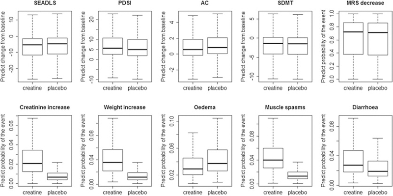
Boxplots of the posterior means of the predicted criteria for all patients in the dataset

To illustrate a personalized BRA, we set aside two patients (denoted as A and B) from the creatine study and predicted their 10 criteria under treatment arm ${\widehat{\mathit{\xi }}}_{Ac}$ and under placebo arm ${\widehat{\mathit{\xi }}}_{Ap}$ as described in Section 3.1. The two patients A and B are same in age (73 years old), gender (male), and race (white) and have similar years of PD symptom, BMI. However, the baseline UPDRS score of patient A is higher than that of patient B (44 vs 21), which indicates a worse disease status of patient A. In the second step, we incorporate patient preference in BRA via individualized SMAA model. We ask the clinician to represent the two patients and to judge the relative importance of the 10 criteria. A weight vector w⁰ is elicited using swing weighting method and presented in Table B1 in Appendix B. For example, improving SEADLS from the worst to the best is $\frac{w_1^0}{w_2^0}=\frac{0.15}{0.10}$ = 1.5 times important than improving PDSI from the worst to the best, considered by the clinician. For demonstration purpose, we assume the weight preferences of patient A and B are well represented by the clinician’s elicitation, ie, w⁰ = ${\mathit{w}}_A^0={\mathit{w}}_B^0,$ but with a large uncertainty, ie, c_A = c_B = 1. We draw 10 000 samples from Dirichlet $\left(c_A\cdot {\mathit{w}}_A^0\right),$ which have the same sample size as predicted criteria. We use the confidence factor c_A = 1 as baseline and conduct the sensitivity analysis on the selection of c_A ∈ [1, 50]. Based on the samples, the utility scores and rank acceptability indices are obtained as described in Section 3.3. The analyses are conducted for patient B in the same fashion.

The rank acceptability indices resulting from the analysis with c_A = c_B = 1 are visualized as bar charts in the panel (A) of Figure 2. The acceptability of creatine as a better treatment for patient A is 0.68. However, placebo is likely to be accepted as a better option by patient B as the first rank acceptability index of creatine is only 0.48. The distributions of the differences in utility scores, creatine compared to placebo, are displayed in panel (B) of Figure 2. The creatine has a slightly better BR balance than placebo for patient A as the median of the score difference is positive. The results of sensitivity analysis of confidence factor c_A and c_B are presented in panel (C) of Figure 2. As the confidence about weight elicitation increases, the first-rank acceptability index for each alternative converges quickly, remaining stable for c_A and c_B greater than 20. Based on the results, physicians are more likely to recommend creatine to patient A, but not patient B. These results may facilitate the decision process for patient A and B, since the suggestions are made based on their personalized response profiles and preferences.

FIGURE 2.

Individualized benefit-risk profile for patient A (first column) and patient B (second column). Panel (A): rank acceptability indices of creatine and placebo at c_A = c_B = 1. Panel (B): distribution of differences in utility scores (creatine vs placebo). Panel (C): first rank acceptability index for each alternative with confidence factor about weight c_A and c_B range from 1 to 50 [Colour figure can be viewed at wileyonlinelibrary.com]

To inform a population-level benefit risk assessment, the similar personalized SMAA procedure are repeated to all the patients in the original dataset. Because the patient preference data was not collected for all subjects, we generate the data and demonstrate the approach via simulation. We introduce individual-level difference in patient preference via sampling initial weights for each patient based on the weights w⁰ and confidence factor c⁰ = 10 elicited by the clinician, ie, ${\mathit{w}}_i^0$ ~ Dirichlet(10w⁰), (i = 1, ..., I), and sample the corresponding confidence factor c_i from an uniform distribution with range [1,10]. Then, the samples are used in SMAA model. The differences in utility scores and the first rank acceptability indices of creatine for each individual patient are calculated and the densities are plotted in Figure 3. As shown in the left panel, for most patients, the difference in utility scores between creatine and placebo is negative, which indicates a lower utility score of creatine when compare to that of placebo. Majority of the patients have the first rank acceptability index of creatine $b_{ic}^1$ less than 0.5 as shown in the right panel. The acceptability of creatine as the best treatment varied among the patients with mean as 0.44, standard deviation as 0.21, and median as 0.44. It suggests that benefit does not outweigh the risk for creatine compared to the placebo for most patients. The reason for this may be that creatine has a limited overall effect on impeding PD progression.¹⁹ However, the personalized BR profile may help to identify a subgroup of patients who may experience greater benefits without associated increase in risks. The patients with $b_{ic}^1$ greater than 0.5, on average, have a higher baseline UPDRS and baseline BMI, compared to patients with $b_{ic}^1$ less than 0.5.

FIGURE 3.

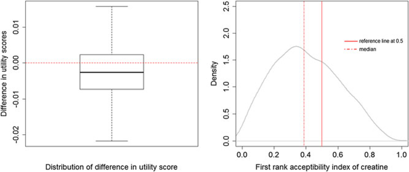
Population-level benefit-risk profile. Left panel: difference in utility scores $\mathrm{\Delta }{\widehat{u}}_i\left({\mathit{\xi }}_{ic},{\mathit{\xi }}_{ip},{\mathit{w}}_i\right)$ of all patients. Right panel: the first rank acceptability index of creatine $b_{ic}^1$ of all patients [Colour figure can be viewed at wileyonlinelibrary.com]

5. DISCUSSION

In this paper, we proposed a novel individual-level multicriteria BRA approach for combining clinical data and patient preference into one value metric. Such a patient-centric approach contributes to the ongoing attempts to integrate patient preference research in medicines assessment. We illustrated how it could facilitates decision-making from patient perspective. Such a focus and approach have not been reported in previous literature.

The proposed MLT-SMAA model allows a combination of statistical data from clinical trials and information from patient preference, with the preference used as weights to scale differences in probability or severity of benefits and risk to reflect their importance to patients. Compared with existing approaches based on group summary data, our model is based on individual-level data that accounts for heterogeneity within the population, thereby enabling more accurate estimates and predictions of the BR balance. Moreover, the proposed approach accounts for the correlation among outcomes through a latent trait model. By introducing two latent variables to represent efficacy and safety domains, respectively, we can assess the association between benefits and risks of the drug. A negative association between the two latent variables may suggest that patients who benefit from treatment may be less likely to experience the specific risks, and considering the individual differences in drug BRA would be necessary. The value of an individual-level BRA is identifying a subgroup of patients, even if a minority, who are most likely to benefit from a product and willing to accept the risk for the benefits it offers.³⁶ This will make the treatment particularly appealing to these subgroups.

There are several limitations and extensions we would like to address in the future work. First, our model relies on a single trial to evaluate the comparative BR profiles of the alternatives. In most cases, the evidence may accumulate from multiple randomized clinical trials and even post-market observational studies, mainly on their safety. This suggests that some form of evidence synthesis is required for the assessment of a treatment’s performance. The proposed MLT model based on a Bayesian generalized mixed model framework can easily incorporate meta-analytical approaches that model study heterogeneity. Second, the proposed method was demonstrated using data at the primary endpoint. However, the trade-off of benefit and risk may change over the course of the trial, especially in long-term trials. To this end, we can extend the proposed MLT model to incorporate the longitudinal outcomes of the patients and enable the criteria prediction for a given patient and SMAA analysis be updated dynamically. Third, we simply use two latent variables to represent efficacy and safety latent states with an underlying assumption of similar behavior of all efficacy outcomes to each other and all safety outcomes to each other. A more objective way of determining the number of latent variables may be based on the pharmaceutical property of a specific drug and need further investigate. However, a larger number of latent variables or even high-dimensional latent variables vector may cause a serious concern of computational time. Future work focusing on variational Bayesian inference or other approximation may address the computational issues. Moreover, the creatine case study was not designed and powered to assess the BR balance of creatine. Rather, it served to illustrate many of the ideas in patient-centered BR using the proposed method in one simplified example. We selected the criteria according to the statistical analysis plan of the original study, the consideration on how to select the efficacy and safety has been thoroughly discussed by many researchers.^37,38 The patient preference was elicited using multicriterial decision analysis swing weighting method in our model. Some practical considerations were discussed in the work of van Valkenhoef and Tervonen.³⁹ Discrete choice experiments is another promising method for capturing patient preferences, which could perform better when sample size is large and the criteria are expected to be easy for the patients to value.⁴⁰ We will investigate other methods for weight elicitation in the future work.

APPENDIX A

TABLE A1.

List of symbols

Notation
K	Number of treatment
J	Number of outcomes or criteria
I	Number of subjects
${\xi }_{ijk}$	Value of criterion j of treatment k on patient i
$u_j\left({\xi }_{ijk}\right)$	Partial value function that normalizes the criterion j
$w_{ij}$	Relative importance of criterion j
$y_{ij}$	Observed value of clinical outcome j of patient i
${\mathit{x}}_i$	Baseline covariates of patient i
$T_{ik}$	Vector of dummy variables that indicates treatment k
${\mathit{w}}_i^0$	Patient preference elicited by patient i
ci	Confidence factor denotes how confidence of patient i about the elicited weight
${\mathit{\theta }}_i$	Subject-specific latent variables shared by all J outcomes
${\mathit{\beta }}_j$	Coefficients of fixed effects on outcome j
${\mathit{\beta }}_{{\mathrm{tr}}_j}$	Coefficients of treatment effect on outcome j
${\mathit{\lambda }}_j$	Latent variable loadings linking ${\mathit{\theta }}_i$ to outcome j
Φ	Vector of unknown parameters
${\xi }_j^{\prime },{\xi }_j^{″}$	The least and most preferable values of criteria j
$u_i({\mathit{\xi }}_{ik},{\mathit{w}}_i)$	Utility score of treatment k on patient i
$\mathrm{\Delta }{u}_i\left({\mathit{\xi }}_{ik},{\mathit{\xi }}_{i{k}^{\prime }},{\mathit{w}}_i\right)$	Difference in utility scores between treatments k and k’ on patient i
$b_{ik}^r$	rth rank acceptability index (r = 1, ..., K) of treatment k on patient i

APPENDIX B

TABLE B1.

Relative importance of the criteria elicited by clinician

	Criteria	Value	Weights (w0)
Efficacy	Schwab and England Activities of Daily Living Scale (SEADLS) CFB	1–100	0.15
	PDQ-39 Summary Index (PDSI) CFB	0–100	0.10
	Ambulatory capacity (AC) CFB	0–20	0.20
	Symbol Digit Modalities Test (SDMT) CFB	0–110	0.10
	Modified Rankin Scale (MRS) decrease	0 or 1	0.10
Safety	Creatinine increase in blood CFB	0 or 1	0.10
	Weight increase	0 or 1	0.05
	Oedema	0 or 1	0.05
	Muscle spasms	0 or 1	0.10
	Diarrhea	0 or 1	0.05

CFB: change from baseline.

• Schwab and England Activities of Daily Living: an assessment of an individual’s ability of function in activities of daily living.

• PDQ-39 Summary Index: test scores indicating the impact of Parkinson’s disease in eight important areas of health status.

• Ambulatory capacity: the sum of five questions from the UPDRS.

• Symbol Digit Modalities Test: screening instrument to assess neurological dysfunction.

• Modified Rankin Scale: measures degree of disability and dependence after a stroke.

REFERENCES

- 1.Mt-Isa S, Hallgreen CE, Wang N, et al. Balancing benefit and risk of medicines: a systematic review and classification of available methodologies. Pharmacoepidemiol Drug Saf. 2014;23(7):667–678. [DOI] [PubMed] [Google Scholar]
- 2.Smith MY, Benattia I, Strauss C, Bloss L, Jiang Q. Structured benefit-risk assessment across the product lifecycle: practical considerations. Ther Innov Regul Sci. 2017;51(4):501–508. [DOI] [PubMed] [Google Scholar]
- 3.Food and Drug Administration. Structured approach to benefit-risk assessment in drug regulatory decision-making. https://www.fda.gov/downloads/forindustry/userfees/prescriptiondruguserfee/ucm329758.pdf. Published 2013. Accessed April 30, 2018.
- 4.Food and Drug Administration. Benefit-risk assessment in drug regulatory decision-making. https://www.fda.gov/downloads/ForIndustry/UserFees/PrescriptionDrugUserFee/UCM602885.pdf. Published 2013. Accessed October 30, 2018.
- 5.European Medicines Agency. Benefit-risk methodology project. Work package 4: Benefit-risk tools and processes. http://www.ema.europa.eu/docs/en_GB/document_library/Report/2012/03/WC500123819.pdf. Published 2012. Accessed April 30, 2018. [Google Scholar]
- 6.Mussen F, Salek S, Walker S. A quantitative approach to benefit-risk assessment of medicines- part 1: the development of a new model using multi-criteria decision analysis. Pharmacoepidemiol Drug Saf. 2007;16(S1):S2–S15. [DOI] [PubMed] [Google Scholar]
- 7.Tervonen T, van Valkenhoef G, Buskens E, Hillege HL, Postmus D. A stochastic multicriteria model for evidence-based decision making in drug benefit-risk analysis. Statist Med. 2011;30(12):1419–1428. [DOI] [PubMed] [Google Scholar]
- 8.Waddingham E, Mt-Isa S, Nixon R, Ashby D. A Bayesian approach to probabilistic sensitivity analysis in structured benefit-risk assessment. Biometrical Journal. 2016;58(1):28–42. [DOI] [PubMed] [Google Scholar]
- 9.van Valkenhoef G, Tervonen T, Zhao J, de Brock B, Hillege HL, Postmus D. Multicriteria benefit-risk assessment using network meta-analysis. J Clin Epidemiol. 2012;65(4):394–403. [DOI] [PubMed] [Google Scholar]
- 10.Wang Y, Mai Y, He W. A quantitative approach for benefit-risk assessment using stochastic multi-criteria discriminatory method. Stat Biopharm Res. 2016;8(4):373–378. [Google Scholar]
- 11.Saint-Hilary G, Cadour S, Robert V, Gasparini M. A simple way to unify multicriteria decision analysis (MCDA) and stochastic multicriteria acceptability analysis (SMAA) using a Dirichlet distribution in benefit-risk assessment. Biometrical Journal. 2017;59(3):567–578. [DOI] [PubMed] [Google Scholar]
- 12.Li K, Yuan SS, Wang W, et al. Periodic benefit-risk assessment using Bayesian stochastic multi-criteria acceptability analysis. Contemp Clin Trials. 2018;67:100–108. [DOI] [PMC free article] [PubMed] [Google Scholar]
- 13.Evans SR, Follmann D. Using outcomes to analyze patients rather than patients to analyze outcomes: a step toward pragmatism in benefit: risk evaluation. Stat Biopharm Res. 2016;8(4):386–393. [DOI] [PMC free article] [PubMed] [Google Scholar]
- 14.Skovlund SE. The potential role of individual-level benefit-risk assessment in treatment decision-making. Ther Innov Regul Sci. 2018. [DOI] [PubMed] [Google Scholar]
- 15.Costa MJ, He W, Jemiai Y, Zhao Y, Di Casoli C. The case for a Bayesian approach to benefit-risk assessment: overview and future directions. Ther Innov Regul Sci. 2017;51(5):568–574. [DOI] [PubMed] [Google Scholar]
- 16.Dunson DB. Bayesian methods for latent trait modelling of longitudinal data. Stat Methods Medical Res. 2007;16(5):399–415. [DOI] [PubMed] [Google Scholar]
- 17.Lee S-Y, Song X- Y. Evaluation of the Bayesian and maximum likelihood approaches in analyzing structural equation models with small sample sizes. Multivar Behav Res. 2004;39(4):653–686. [DOI] [PubMed] [Google Scholar]
- 18.Cooper R, Naclerio F, Allgrove J, Jimenez A. Creatine supplementation with specific view to exercise/sports performance: an update. J. Int Soc Sports Nutr. 2012;9(1):33. [DOI] [PMC free article] [PubMed] [Google Scholar]
- 19.Kieburtz K, Tilley BC, Elm JJ, et al. Effect of creatine monohydrate on clinical progression patients with Parkinson disease. JAMA. 2015;313(6):584–593. [DOI] [PMC free article] [PubMed] [Google Scholar]
- 20.Keeney RL, Raiffa H. Decisions With Multiple Objectives: Preferences and Value Trade-Offs. Cambridge, UK: Cambridge University Press; 1993. [Google Scholar]
- 21.Dunson DB. Bayesian latent variable models for clustered mixed outcomes. J Royal Stat Soc SerB Stat Methodol. 2000;62(2):355–366. [Google Scholar]
- 22.Lazarsfeld PF. Latent structure analysis. Psychol Study Sci. 1959;3:476–543. [Google Scholar]
- 23.Dunson DB. Dynamic latent trait models for multidimensional longitudinal data. J Am Stat Assoc. 2003;98(463):555–563. [Google Scholar]
- 24.Teixeira-Pinto A, Normand S-LT. Correlated bivariate continuous and binary outcomes: issues and applications. Statist Med. 2009;28(13):1753–1773. [DOI] [PMC free article] [PubMed] [Google Scholar]
- 25.Wang J, Luo S, Li L. Dynamic prediction for multiple repeated measures and event time data: An application to parkinson’s disease. Ann Appl Stat. 2017;11(3):1787. [DOI] [PMC free article] [PubMed] [Google Scholar]
- 26.Wang J, Luo S. Multidimensional latent trait linear mixed model: an application in clinical studies with multivariate longitudinal outcomes. Statist Med. 2017;36(20):3244–3256. [DOI] [PMC free article] [PubMed] [Google Scholar]
- 27.Thokala P, Devlin N, Marsh K, et al. Multiple criteria decision analysis for health care decision making-an introduction: report 1 of the ISPOR MCDA emerging good practices task force. Value Health. 2016;19(1):1–13. [DOI] [PubMed] [Google Scholar]
- 28.Von Winterfeldt D, Edwards W. Decision Analysis and Behavioral Research. Cambridge, UK: Cambridge University Press; 1993. [Google Scholar]
- 29.Watson SR, Buede DM. Decision Synthesis: The Principles and Practice of Decision Analysis. Cambridge, UK: Cambridge University Press; 1987. [Google Scholar]
- 30.Clemen RT, Reilly T. Making Hard Decisions with Decision Tools. Mason, OH: Cengage Learning; 2013. [Google Scholar]
- 31.Lunn D, Spiegelhalter D, Thomas A, Best N. The BUGS project: evolution, critique and future directions. Statist Med. 2009;28(25):3049–3067. [DOI] [PubMed] [Google Scholar]
- 32.Hornik K, Leisch F, Zeileis A. JAGS: a program for analysis of Bayesian graphical models using Gibbs sampling. In: Proceedings of the 3rd International Workshop on Distributed Statistical Computing (DSC 2003); 2003; Vienna, Austria. [Google Scholar]
- 33.NealRM. MCMC using hamiltonian dynamics In: Handbook of Markov Chain Monte Carlo. Vol. 2 Boca Raton, FL: Chapman & Hall/CRC; 2011:113–162. [Google Scholar]
- 34.Hoffman MD, Gelman A. The No-U-Turn sampler: adaptively setting path lengths in Hamiltonian Monte Carlo. J Mach Learn Res. 2014;15(1):1593–1623. [Google Scholar]
- 35.Gelman A, Carlin JB, Stern HS, Rubin DB. Bayesian Data Analysis. New York, NY: CRC Press; 2013. [Google Scholar]
- 36.Food and Drug Administration. Medical device innovation consortium (MDIC) patient centered benefit-risk project report. https://www.fda.gov/downloads/ScienceResearch/SpecialTopics/RegulatoryScience/UCM486253.pdf. Published 2013. Accessed April 10, 2019.
- 37.Tervonen T, Naci H, van Valkenhoef G, et al. Applying multiple criteria decision analysis to comparative benefit-risk assessment: choosing among statins in primary prevention. Med Decis Mak. 2015;35(7):859–871. [DOI] [PubMed] [Google Scholar]
- 38.Ma H, Jiang Q, Chuang-Stein C, et al. Considerations on endpoint selection, weighting determination, and uncertainty evaluation in the benefit-risk assessment of medical product. Stat Biopharm Res. 2016;8(4):417–425. [Google Scholar]
- 39.van Valkenhoef G, Tervonen T. Entropy-optimal weight constraint elicitation with additive multi-attribute utility models. Omega. 2016;64:1–12. [Google Scholar]
- 40.Tervonen T, Gelhorn H, Sri Bhashyam S, et al. MCDA swing weighting and discrete choice experiments for elicitation of patient benefit-risk preferences: a critical assessment. Pharmacoepidemiol Drug Saf. 2017;26(12):1483–1491. [DOI] [PubMed] [Google Scholar]
Associated Data
This section collects any data citations, data availability statements, or supplementary materials included in this article.