

Supplemental Digital Content is available in the text.
Keywords: Asymmetric penalty, Bivariate smoothing, Constrained P-splines, Incidence monitoring, Infectious disease outbreaks, Nowcasting
Abstract
During an infectious disease outbreak, timely information on the number of new symptomatic cases is crucial. However, the reporting of new cases is usually subject to delay due to the incubation period, time to seek care, and diagnosis. This results in a downward bias in the numbers of new cases by the times of symptoms onset towards the current day. The real-time assessment of the current situation while correcting for underreporting is called nowcasting. We present a nowcasting method based on bivariate P-spline smoothing of the number of reported cases by time of symptoms onset and delay. Our objective is to predict the number of symptomatic-but-not-yet-reported cases and combine these with the already reported symptomatic cases into a nowcast. We assume the underlying two-dimensional reporting intensity surface to be smooth. We include prior information on the reporting process as additional constraints: the smooth surface is unimodal in the reporting delay dimension, is (almost) zero at a predefined maximum delay and has a prescribed shape at the beginning of the outbreak. Parameter estimation is done efficiently by penalized iterative weighted least squares. We illustrate our method on a large measles outbreak in the Netherlands. We show that even with very limited information the method is able to accurately predict the number of symptomatic-but-not-yet-reported cases. This results in substantially improved monitoring of new symptomatic cases in real time.
During outbreaks of diseases such as ebola,1 zika,2 chikungunya,3 measles,4 pandemic influenza5 or large food-borne disease outbreaks,6,7 international or federal governmental institutes are responsible for disease control and prevention. They have the task of monitoring the number of new symptomatic cases by time of disease onset in order to inform relevant health authorities, assess the severity of the current situation, and assess the impact of possible control measures.
However, the reporting of symptomatic cases is usually subject to delay between the time of symptoms onset and the time that the case is reported. A consequence is that the numbers of new cases by the times of symptoms onset show a downward bias towards the current day.
Depending on the type of infection and on the health reporting system, the reporting delay varies between several days (e.g., for influenza) to several months (e.g., for tuberculosis). The reporting delay is caused by various controllable and uncontrollable processes, such as the incubation period of the infection, the time patients wait to seek care, the time between submission of a sample and laboratory confirmation and the time to final report by the health department in the database.8,9 Furthermore, often a strong day-of-the-week effect is present: very few cases are reported on Saturdays and Sundays.
The assessment of the current situation based on imperfect or partial information is called nowcasting.10 When the distribution function of the reporting delay is known, it is possible to obtain a point estimate of the number of new symptomatic cases in real time, e.g., by simply dividing the number of already reported cases by the fraction of reported cases at the current day, yesterday, etc. In practice, however, it is very difficult to obtain stable estimates of the number of new cases on a daily basis. This is particularly true when the number of reported cases is low, or even zero, and when the fraction of reported cases is low. Moreover, at the beginning of the outbreak, little information is known about the shape of the reporting delay distribution, and the information there is biased towards shorter delays because cases with longer delays have not been reported yet. Furthermore, the reporting delay distribution can change over time.11,12
Statistical modeling techniques can make an improvement here. A good overview of available nowcast models is provided by Höhle and an der Heiden.12 As an alternative to existing models, they introduce a joint modeling approach that simultaneously estimates the time-varying reporting delay distribution and makes a prediction of the epidemic curve. The reporting delay distribution is modeled by a time-dependent discrete time-to-event model, while a penalized spline smoothing approach is used to provide a stable estimate of the epidemic curve. A drawback of such an approach is the complexity of the model, which requires estimation in a Bayesian framework using Markov Chain Monte Carlo, leading inevitably to long computation times, often too long for inclusion in regular monitoring tools.
We propose an alternative approach based on penalized likelihood estimation in the frequentist framework.13 First, the numbers of reported cases are organized in a lower triangular contingency table, with on one margin the time of symptoms onset and on the other the reporting delay. This is the so-called reporting triangle.11 Next, we impose a maximum to the reporting delay, where we can safely assume that all cases have been reported. The reporting triangle then becomes a trapezoid. Our objective is to make a fast and accurate prediction of the number of symptomatic-but-not-yet-reported cases in the upper triangular part of the contingency table and combine these with the already reported symptomatic cases by time of symptoms onset into a nowcast.
Instead of a time-to-event approach, we directly model the number of symptomatic cases in the reporting trapezoid. We assume that the underlying reporting intensity is a smooth surface, with day-of-the-week effects expressed as deviations from it. The two-dimensional surface is modeled using bivariate P-splines.14 P-splines are penalized B-splines and provide a flexible way to smooth data and extrapolate trends.15,16 However, to obtain a stable extrapolation of the surface outside the reporting trapezoid, especially at the beginning of the outbreak, we include prior information on the reporting process as additional constraints: the surface is unimodal in the reporting delay dimension, is (nearly) zero at the predefined maximum delay, and has a presumed shape at the beginning of the outbreak. The advantage of this approach is that it is intuitive and fast.
We apply our method to a large measles outbreak in the Netherlands in 2013–2014 and investigate its performance in different stages of the outbreak.
METHODS
Constructing the Two-dimensional Contingency Table
We describe the infection process and observations process, following the notation of Höhle and an der Heiden.12 We first organize the number of cases in a two-dimensional contingency table, with on one margin the time of symptoms onset 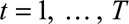 days, starting on day 1 of the outbreak and on the other margin the reporting delay
  days. Thus
  is the current day (the “now”) in the outbreak and
  is the predefined maximum delay.
Figure 1 shows a schematic representation of such a two-dimensional contingency table for  and
and  . The (
 )-cell of the table represents the number of cases, denoted by
  , occurring at time
  and reported with a delay of
  , and corresponds to a certain day of the week. For a given report date
  is constant.
FIGURE 1.
Schematic representation of a two-dimensional contingency table for the number of cases. Horizontal axis: time of symptoms onset t. Vertical axis: reporting delay d. Here the current time of symptoms onset is  and the predefined maximum delay is D = 3. Blue: reporting trapezoid, i.e., number of symptomatic cases that have been reported. Orange: number of symptomatic cases that have not been reported yet (to be predicted). Gray: cases without symptoms and consequently not reported (future).
  is the total number of cases by time of symptoms onset.
We distinguish three types of cases: (1) Cases with  have symptoms and have been reported. This is the reporting trapezoid (blue). (2) Cases with
  have symptoms, but have not been reported yet (orange). These cases are right truncated. (3) Cases with
  do not have symptoms yet, because they occur in the future (gray). Note that these numbers are only known in retrospect.
The objective of nowcasting is to predict the total number of cases  for times of symptoms onset
  . This number is given by
  . We therefore have to combine the already reported symptomatic cases in the reporting trapezoid with a prediction of the number of symptomatic-but-not-yet-reported cases in the upper triangular part of the contingency table.
Modeling the Number of Reported Cases
We consider the number of reported cases by time of symptoms onset and delay as known and the number of symptomatic-but-not-yet-reported cases as missing values. The model formulation below allows prediction of the number of symptomatic-but-not-yet-reported cases simultaneously with the estimation procedure. See the section on parameter estimation.
Observations suggest that counts are usually overdispersed, i.e., have a variance greater than the mean. We therefore assume that number of reported cases by time of symptoms onset and delay follows a Negative Binomial distribution with mean  , the reporting intensity, and overdispersion parameter
  :
:
| (1) |
The variance is given by  . For
. For  , the distribution approaches a Poisson distribution, which was used by Höhle and an der Heiden.12 The reporting intensity
  is related to a linear predictor through the log link function, in order to keep the reporting intensity positive.
The linear predictor consists of two parts. We assume that the reporting intensity is a two-dimensional smooth surface in the time of symptoms onset and delay dimension (first part), with day-of-the-week effects expressed as deviations from this surface (second part). The assumption of smoothness comes from the idea that the data generating process, apart from day-of-the-week effects, varies gradually over the time of symptoms onset and in the reporting delay direction.
To achieve the first part, i.e., the smooth two-dimensional surface, the effect of time of symptoms onset on the reporting intensity is modeled by a linear combination of  basis functions
  , where
  is a set of unknown regression coefficients with
  . A similar expression applies to the reporting delay.
We use B-spline basis functions. B-splines are piecewise polynomials of a given degree, usually cubic, which are fused smoothly in a pre-specified number of equidistant knots. The main advantage of the B-splines basis is its local definition, i.e., being zero everywhere, except on an interval around a knot,15 favorable over, e.g., polynomial splines and truncated power series, which may lead to numerical instabilities.17
The time of symptoms onset and reporting delay need not to be independent. To model the full interaction, we use a tensor product B-spline basis. Such a basis is obtained by considering all pairwise products  of the two univariate bases constructed for univariate smooths.14,17
The second part of the linear predictor is the day-of-the-week effect, expressed as deviations from the smooth surface. We can write these deviations as a set of  dummy variables, taking the value 1 if a certain combination of
  and
and  corresponds to a given day of the week and 0 otherwise.
Taking the smooth surface and the deviations from it together, the linear predictor is written as:
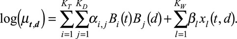 |
(2) |
Here  and
and  are the univariate B-spline basis functions of respectively time of symptoms onset and delay. The number of knots is provided by
  and
and  . Controlling the roughness of the surface will be dealt with later. Furthermore,
  , with
  , represent the day-of-the-week effects, as described above. Monday is taken as a reference and is implicitly included in the smooth trend surface, hence
  .
.
For the purpose of regression, we arrange the data from grid to column order and switch to matrix notation. The first double summation can now be written as  , where
  . The symbol
  represents the Kronecker or tensor product of the two univariate B-splines matrices
  and
and  with dimensions
  and
and  , respectively. Consequently,
  is a matrix with dimension
  . α is a vector of the corresponding regression coefficients.
The second term can be written as  , where
  is a binary-valued matrix with dimension
  .
.  is a vector of the corresponding regression coefficients.
Imposing Constraints
In order to obtain stable estimates of both the smooth surface and the day-of-the-week effect, we include prior information on the reporting process as additional constraints: the surface is unimodal in the reporting delay dimension, is (nearly) zero at the predefined maximum delay, and has a presumed shape at the beginning of the outbreak. Furthermore, the regression coefficients  are regularized to avoid extreme estimates in a sparse data setting. The mathematics behind these constraints can be found in the eMethods; http://links.lww.com/EDE/B544 section in the supplementary material. There we show in detail how the constraints are constructed and how they are applied as penalizations on the Negative Binomial log-likelihood function
  .
.
Parameter Estimation
The smooth surface and the day-of-the-week effects are estimated simultaneously. We can write our method as a penalized generalized linear model, with a Negative Binomial error distribution, a log-link function, a model matrix and, additionally, a penalty matrix. We can therefore use the penalized version of the iterative weighted least squares algorithm. Details can be found in the eMethods; http://links.lww.com/EDE/B544 section in the supplementary material.
Nowcasting
Once the regression coefficients  and
and  and overdispersion parameter
  have been estimated (including their covariance matrix), the nowcast can be produced. As it is not straightforward to write down closed-form equations, we use Monte Carlo simulation to deal with the parameter uncertainties and the generation of prediction intervals.
(1) Generate 1000 Monte Carlo samples for the regression coefficients. We assume that the estimates follow a multivariate Normal distribution. We empirically found that 1000 samples are enough.
(2) Calculate the expected reporting intensity for the symptomatic cases that have not been reported yet: for each realization of
 and
and  , calculate
  for
for  using equation (2).
(3) Generate the number
 of symptomatic cases that have not been reported yet: for each realization of
  and
and  , sample one realization from the Negative Binomial distribution using equation (1), resulting again in 1000 Monte Carlo samples.
(4) Summarize the number of symptomatic cases by time of symptoms onset: for each realization of
 , calculate
 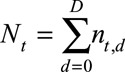 for
for 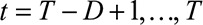 . This procedure combines the already reported symptomatic cases with the predicted number of symptomatic-but-not-yet-reported cases from step 3.
(5) For each time of symptoms onset, compute the empirical predictive distribution function. From this, any desired statistics, such as the median or prediction interval, can be computed. It can also be used to evaluate the nowcast in retrospect.
Evaluating the Nowcast Performance
We assessed performance by comparing the predictive distribution for new symptomatic cases with the observed number by time of symptoms onset  . We investigated three different phases in an outbreak: (1) the growth phase, usually characterized by a positive exponential epidemic growth rate in the number of cases, (2) the peak phase, characterized by a near zero growth rate, and (3) the decline phase of the outbreak, characterized by a negative exponential growth rate. Furthermore, we investigated the effect of the order of the differences
  on the coefficients in the time of symptoms onset dimension. See the eMethods; http://links.lww.com/EDE/B544 section in the supplementary material for more details on these difference orders. Our default setting,
  , results in a linear extrapolation of epidemic trends on a log-scale. However, sometimes this resulted in overshooting of trends. Hence, we also set
  and see how well our method performs.
We evaluated the nowcasts by using the probability integral transform (PIT) histogram.18 This histogram is especially useful for probabilistic forecasts (nowcasts in our case). A probabilistic forecast does not have one outcome, but a range of outcomes, each with its own probability. If observations were drawn from the predictive distribution, the PIT histogram should show a uniform distribution. Deviations from uniformity indicate model deficiencies. For example, skewness towards higher (lower) PIT values indicates that the observations are too high (low) compared to the predictive distribution. In other words, the nowcast underestimates (overestimates) the true epidemic curve.
Time-varying Reporting Delay Distribution
In can be of interest to have an estimate of the time-varying distribution of reporting delays. This can be obtained using the first term in equation (2):
(1) Calculate the contribution of the bivariate smoothing term to the reporting intensity: given the estimated regression coefficients
 , calculate
  = exp(
 ) for all combinations of
 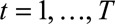 and
and 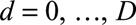 . Superscript
  denotes the smooth surface.
(2) Arrange
 back into a
  grid,
grid,  .
.(3) Calculate the time-varying reporting delay distribution (probability mass function) by normalizing
 on its column totals:
  , for
, for  .
.
The day-of-the-week effect is ignored to obtain a smooth estimate. Since Monday is taken as the reference day of the week, the smooth surface for any other day is multiplied by a factor equal to the exponent of the corresponding regression coefficient for that day. This factor cancels out by conditioning on column totals. However, one could still include the day-of-the-week effect in the reporting delay distribution if desired by replacing  by
by  .
.
NOWCASTING A LARGE MEASLES OUTBREAK IN THE NETHERLANDS
Data
During May 2013–March 2014, the Netherlands was affected by a large measles outbreak.4,19 The outbreak commenced in the center of the country in an orthodox protestant community and spread to regions with low vaccination coverage. Two thousand seven hundred patients with measles have been reported, 181 children were hospitalized and one child died from complications of measles. The first case occurred on 8 May 2013; however it was not reported until 27 May, with a delay of 19 days, together with five other cases.
Figure 2 shows the number of cases by symptoms onset time on Saturday 10 August 2013. This is 1 month after the peak of the outbreak. We have complete data on the entire outbreak in retrospect (only the reported symptomatic cases). In the top panel, the blue bars show the number of symptomatic cases that have been reported up to 10 August 2013. The orange bars show the number of symptomatic cases that have not been reported yet up to 10 August 2013. The gray bars show the number of cases with symptoms onset time after 10 August 2013.
FIGURE 2.
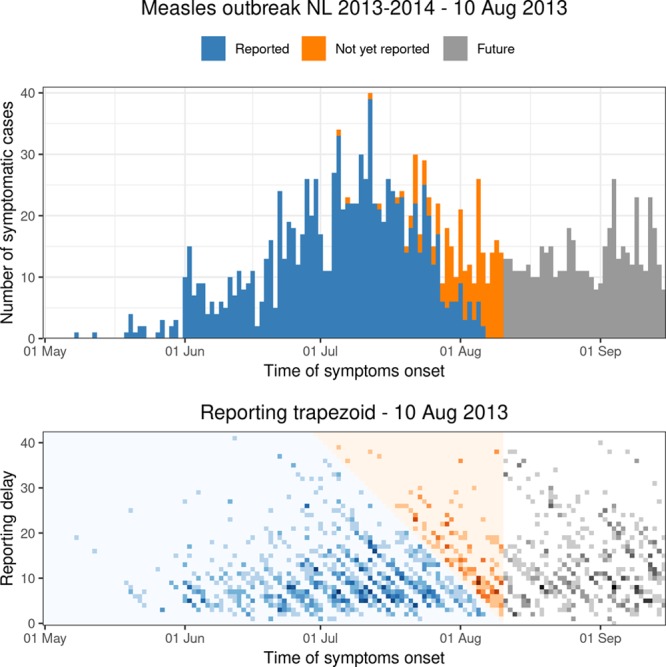
Top panel: daily number of symptomatic cases during the Measles outbreak in the Netherlands for the period 1 May–15 September 2013, as available in retrospect. Bottom panel: corresponding reporting trapezoid. Blue colors: reported symptomatic cases up to 10 August 2013. Orange colors: not yet reported symptomatic cases on 10 August 2013. Gray colors: cases without symptoms (future).
The bottom panel visualizes the corresponding two-dimensional contingency table. The meaning of the colors is the same as in the top panel. The darker the colors, the more cases are being reported for that specific combination of time of symptoms onset and reporting delay. Day-of-the-week effects can be recognized as diagonal patterns running from the top left to the bottom right. Hardly any cases were reported in weekends, as suggested by the lighter diagonal band structures. Our objective is to model the number of reported symptomatic cases in the blue reporting trapezoid and predict the number of symptomatic-but-not-yet-reported cases in the orange upper triangular part of the contingency table. Both are provided by the nowcast.
Model Setup
From Figure 2, we can distinguish the following three phases in the outbreak: (1) Growth phase: June 2013. (2) Peak phase: July 2013. (3) Decline phase: August 2013. To illustrate our method, we produced nowcasts for three specific dates: 10 June 2013 (growth phase), 10 July 2013 (peak incidence), and 10 August 2013 (decline phase). We considered 1 May 2013 as day 1 ( ).
).
Next, we had to translate prior information on the reporting process into constraints for our nowcast model. See the eMethods; http://links.lww.com/EDE/B544 section in the supplementary material for more details. We had to define the boundary constraints at  and
and  . From our database, for measles reports before 1 May 2013, we found that the average reporting delay was 12 days and that 99% of all cases were being reported within 6 weeks (42 days).8 By setting this maximum, we lose a few cases (1%) with longer reporting delays, but this had no consequences for the results. Assuming a Negative Binomial reporting delay distribution, these numbers defined the boundary constraint at
  and
and 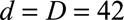 days.
days.
Furthermore, we penalized second order differences of the regression coefficients in the time of symptoms onset dimension (mT = 2), so any possible trends in that dimension will be extrapolated linearly (on a log-scale). We did the same for the reporting delay distribution dimension (mD = 2). We took the default fixed parameters κu = 106, κb = 106, κw = 0.01, and κs = 10−6. See the eMethods; http://links.lww.com/EDE/B544 section in the supplementary material for more details.
In practice it is usually not necessary to include all times of symptoms onset  , so one option of the model is to set a time window to be used in the estimation procedure. By default, this window is set to
  , in our case a window of 12 weeks (84 days).
RESULTS
Figure 3 shows the nowcasts on 10 June, 10 July, and 10 August 2013. The blue bars show the number of symptomatic cases that had been reported up to that date. The gray bars show the number of symptomatic cases that had not been reported yet. The orange lines are the nowcasts (median) and the orange shaded areas are the 90% prediction intervals.
FIGURE 3.
Nowcast of the Measles outbreak for 10 June, 10 July, and 10 August 2013 to 6 weeks back (orange colors). The shaded areas are the 90% prediction intervals.
In general, although very few cases, or even zero cases, have been reported on the days before each nowcast date, the model is still able to predict the number of symptomatic-but-not-yet-reported cases quite well. As we go further back in time, more symptomatic cases are being reported. As a result, the prediction interval gets narrower. More specifically, if we look in at June 10, only a limited number of cases have been reported up to that date. Based on these observations and prior information on the reporting process, the nowcasting method seems to overestimate the true number of symptomatic cases during this phase of the outbreak. If we look specifically at 10 July and 10 August, the method seems to capture the epidemic trends better. The performance will be formally assessed in the next section.
Figure 4 shows the smooth time-varying distribution of reporting delays. For illustrating the time-varying nature of the reporting process, it includes all times of symptoms onset from  up to 1 September 2013. The orange triangle is the extrapolation based on the available data in the reporting trapezoid. At the beginning of the outbreak, the distribution is mainly defined by the boundary constraint at
  . As more information becomes available, a gradual shift towards shorter delays can be seen, resulting in a more peaked distribution in June 2013. The highest reporting intensities occur with a delay of 5–9 days. In July and August, the reporting delays get less concentrated, possibly because of the holidays resulting in longer waiting times to contact a general practitioner or understaffing at the Municipal Health Services.
FIGURE 4.
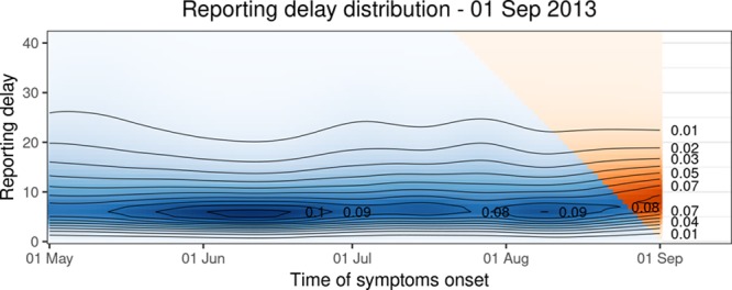
Time varying reporting delay distribution up to 1 September 2013. The blue colors indicate the smoothed distribution based on the observations. The extrapolation is indicated by orange colors. The contour lines indicate levels of equal probability mass.
eFigure 1 (Supplementary material; http://links.lww.com/EDE/B544) shows the estimated day-of-the-week effects as rate ratios (RR) including 95% confidence intervals for the nowcast date 10 August 2013. Because Monday is taken as the reference day, RR = 1 for this day. Monday is also the day with the highest reporting rate, probably because of the weekend cases being reported then. There is a decrease in reporting rates during weekdays, except for Friday, which is comparable to Mondays. During weekends hardly any cases are being reported, resulting in rate ratios near zero, compared to Mondays.
Performance
We assessed the nowcast performance during 15 days within each of the three outbreak phases. More specifically, for example for the growth phase, around 10 June, from 3 June to 17 June, etc. Because we are most interested in good performance in real-time, i.e., close to the current day during the outbreak, nowcasts are being produced to 7 days back, starting at the current day, i.e., 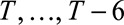 . For each date we compare the predictive distribution with the true number of reported cases
  . Subsequently, we let
  run within each phase of the outbreak. Note that the observed value
  is being used multiple times. Hence, each PIT histogram is based on 7 × 15 = 105 days. The included times of symptoms onset in the estimation procedure are set to the default, which is twice the maximum reporting delay, here 12 weeks (84 days).
The corresponding PIT histograms are shown in eFigure 2 (Supplementary material; http://links.lww.com/EDE/B544). The columns show the growth phase, peak phase, and decline phase of the outbreak; the rows show the effect of penalization of the first order and second order differences on the adjacent coefficients in the time of symptoms onset dimension.
During the initial phase (10 June 2013 ± 7 days), taking first order differences, the histogram shows a tendency to higher PIT values. This indicates that the predictive distribution is most of the time too low compared to the observed numbers. Taking second order differences, the PIT histogram shows a tendency to lower PIT values, indicating that the predictive distribution is too high compared to the observed numbers, which corresponds the upper panel in Figure 2. If we calculate the mean absolute difference the bars with one (dashed horizontal line), it is 0.84 for the first order differences and 0.70 for the second order differences, indicating that taking second order differences is better.
During the peak phase (10 July 2013 ± 7 days), taking first order differences, again results in a predictive distribution that is too low compared to the observed numbers. Taking second order differences, the PIT histogram is more or less uniform. Here the nowcast performs better than during the growth phase. For the second order differences this corresponds to what we see in the middle panel in Figure 2. The mean absolute difference is 0.87 for the first order differences and 0.23 for the second order differences.
During the decline phase (10 August 2013 ± 7 days), there seems to be a tendency to lower PIT values, both taking first and second order differences. This indicates that the predictive distribution is most of the time a bit too high compared to the observed numbers. For the second order differences this corresponds to what we see in the lower panel in Figure 2. The mean absolute difference is 0.72 for the first order differences and 0.62 for the second order differences.
DISCUSSION
During an infectious disease outbreak, it is important to have real-time information on the number of new symptomatic cases. Because of reporting delays, relying only on reported cases will result in biased estimates for the most recent time. We have shown how to combine information from already reported cases with a nowcast model to make real-time predictions. These predictions can be used for outbreak management.
The advantage of our nowcasting method is that it is intuitive and fast. It is intuitive as it considers a direct modeling of the number of cases in the dimensions of symptoms onset time and reporting delay. Prior information about the reporting process is included in the model by translating it into additional constraints. Subsequently, the two-dimensional surface is extrapolated outside the reporting trapezoid. The method is computationally fast as it can be thought of as a penalized generalized linear model. This allows model building in terms of a regression matrix, an error distribution, and a link function. Although penalties are added, the algorithm retains the efficient iterative weighted least squares form. Estimation is done in seconds. This allows it to be used in real-time monitoring.
The method has many similarities with the Bayesian hierarchical approach of Höhle and an der Heiden,12 like modeling counts in the reporting trapezoid, taking the right truncation of the reporting process into account, smoothing the epidemic trend in the dimension of symptoms onset time, and allowing incorporation of covariates, here day-of-the-week effects. However, using our approach, modeling sudden changes in the reporting process can be challenging. Currently, any sudden changes in the reporting process will be manifested as gradual trends in the reporting intensity surface. However, by setting specific elements in difference operator matrices to zero, breaks or jumps can be incorporated. Furthermore, a sudden change could be incorporated as a categorical covariate in the regression framework. For the measles outbreak we have seen that the reporting delay distribution was slightly time-varying. The model was able to pick up these gradual changes.
The constraints that are introduced reflect prior information on the reporting process, which we consider important to take into account. Without these constraints, it was almost impossible to generate a stable extrapolation outside the reporting trapezoid. The most important constraint is the boundary constraint. It forces the smooth reporting intensity surface below prespecified values. Here, these values were based on historical knowledge of the reporting process, but an educated guess could have been used as well. It should be noted that if only a few cases can be expected at  , then this information should certainly be included, or else the fit will become very unstable because of the few observations. However, if already many cases can be expected at
  , then this constraint becomes less important because there are enough observations to inform the model. In the beginning of an outbreak one can use reporting delays from previous outbreaks to get some idea about the expected delays and about a maximum reporting delay during the current outbreak.
Of lesser importance is the unimodality constraint. This is because most of the time, though not always, the boundary constraint at  already results in a unimodal stable extrapolation outside reporting trapezoid. Furthermore, for some diseases, the reporting delay distribution will not always be unimodal, e.g. for tuberculosis or HIV, which typically have long variable reporting delays. For such diseases, by simply setting
  , the unimodality constraint can be disabled in our nowcasting method. See the eMethods section in the supplementary material for more details.
Parameter uncertainty is taken into account in the nowcasting procedure by Monte Carlo sampling. In addition, the prediction interval is obtained by Monte Carlo sampling. This allows generating a predictive empirical distribution function for each date. Furthermore, knowing the true number of cases by date in retrospect allows evaluating the quality of the nowcasts, using PIT histograms.
We evaluated the nowcasts for three phases during the outbreak. We chose these phases to investigate the behavior of the method under different circumstances. We chose the length of the period, 7 days backward, in a 15-day moving window, to evaluate the nowcast performance in real-time, i.e., close to the current day during an outbreak. Based on the mean absolute differences of the PIT values compared to one, taking second-order differences resulted in a better performance. However, during the growth phase of the outbreak the predictive distribution then is too high, compared to the observed numbers. During the peak and decline phase, the nowcast performed better.
Future work involves the implementation the generalized linear array model algorithm20 to further increase the computational efficiency. Furthermore, the model formulation can be generalized, so that more covariates, in addition to the day of the week, can easily be incorporated. In addition, the possibility to include breaks or jumps should be further investigated. Finally, it would be interesting to investigate other diseases with much longer reporting delays, e.g., pertussis, having an average delay of several weeks.8
CONCLUSIONS
We have presented a nowcasting method for estimating the number of new symptomatic cases during infectious disease outbreaks. In essence, we estimate a two-dimensional reporting intensity surface and extrapolate this surface to predict the number of symptomatic-but-not-yet-reported cases. Our method directly models the reported number of cases by symptoms onset time and reporting delay using P-splines. Prior information on the reporting process is included as additional constraints. The extrapolation, in combination with the number of already reported symptomatic cases, allows constructing a nowcast for the current day and backwards, up to a predefined maximum delay. Even with very limited information, the method is able to predict the number of symptomatic-but-not-yet-reported cases quite well. The method is fast, which allows it to be used in real-time monitoring.
Supplementary Material
Footnotes
The authors report no conflicts of interest.
Replication of results: Data and R scripts to reproduce the results can be found on https://github.com/kassteele/Nowcasting.
Supplemental digital content is available through direct URL citations in the HTML and PDF versions of this article (www.epidem.com).
REFERENCES
- 1.Aylward B, Barboza P, Bawo L, et al. ; WHO Ebola Response Team. Ebola virus disease in West Africa–the first 9 months of the epidemic and forward projections. N Engl J Med. 2014;371:1481–1495. [DOI] [PMC free article] [PubMed] [Google Scholar]
- 2.Lessler J, Chaisson LH, Kucirka LM, et al. Assessing the global threat from zika virus. Science. 2016;353:aaf8160. [DOI] [PMC free article] [PubMed] [Google Scholar]
- 3.Cauchemez S, Ledrans M, Poletto C, et al. Local and regional spread of chikungunya fever in the Americas. Euro Surveill. 2014;19:20854. [DOI] [PMC free article] [PubMed] [Google Scholar]
- 4.Woudenberg T, van Binnendijk RS, Sanders EAM, et al. Large measles epidemic in the Netherlands, may 2013 to March 2014: changing epidemiology. Euro Surveill. 2017;22:30443. [DOI] [PMC free article] [PubMed] [Google Scholar]
- 5.Dawood FS, Iuliano AD, Reed C, et al. Estimated global mortality associated with the first 12 months of 2009 pandemic influenza A H1N1 virus circulation: a modelling study. Lancet Infect Dis. 2012;12:687–695. [DOI] [PubMed] [Google Scholar]
- 6.Buchholz U, Bernard H, Werber D, et al. German outbreak of Escherichia coli O104:H4 associated with sprouts. N Engl J Med. 2011;365:1763–1770. [DOI] [PubMed] [Google Scholar]
- 7.Friesema I, Jong A, de, Hofhuis A, et al. Large outbreak of salmonella thompson related to smoked salmon in the Netherlands, August to December 2012. Eurosurveillance. 2014;19:20918. [DOI] [PubMed] [Google Scholar]
- 8.Marinović AB, Swaan C, van Steenbergen J, Kretzschmar M. Quantifying reporting timeliness to improve outbreak control. Emerg Infect Dis. 2015;21:209–216. [DOI] [PMC free article] [PubMed] [Google Scholar]
- 9.Noufaily A, Ghebremichael-Weldeselassie Y, Enki DG, et al. Modelling reporting delays for outbreak detection in infectious disease data. J R Stat Soc Ser A Stat Soc. 2015;178:205–222. [Google Scholar]
- 10.Donker T, van Boven M, van Ballegooijen WM, van’t Klooster TM, Wielders CC, Wallinga J. Nowcasting pandemic influenza A/H1N1 2009 hospitalizations in the Netherlands. Eur J Epidemiol. 2011;26:195–201. [DOI] [PMC free article] [PubMed] [Google Scholar]
- 11.Lawless JF. Adjustments for reporting delays and the prediction of occurred but not reported events. Can J Stat Rev Can Stat. 1994;22:15–31. [Google Scholar]
- 12.Höhle M, an der Heiden M. Bayesian nowcasting during the STEC O104:H4 outbreak in Germany, 2011. Biometrics. 2014;70:993–1002. [DOI] [PubMed] [Google Scholar]
- 13.Cole SR, Chu H, Greenland S. Maximum likelihood, profile likelihood, and penalized likelihood: a primer. Am J Epidemiol. 2014;179:252–260. [DOI] [PMC free article] [PubMed] [Google Scholar]
- 14.Eilers PHC, Marx BD. Multivariate calibration with temperature interaction using two-dimensional penalized signal regression. Chemom Intell Lab Syst. 2003;66:159–174. [Google Scholar]
- 15.Eilers PHC, Marx BD. Flexible smoothing with B-splines and penalties. Stat Sci. 1996;11:89–121. [Google Scholar]
- 16.Eilers PHC, Marx BD, Durbán M. Twenty years of P-splines. SORT-Stat Oper Res Trans. 2015;39:149–186. [Google Scholar]
- 17.Fahrmeir L, Kneib T, Lang S, Marx B. Regression; Models, Methods and Applications. 2013Berlin, Heidelberg: Springer Berlin Heidelberg. [Google Scholar]
- 18.Czado C, Gneiting T, Held L. Predictive model assessment for count data. Biometrics. 2009;65:1254–1261. [DOI] [PubMed] [Google Scholar]
- 19.Knol M, Urbanus A, Swart E, et al. Large ongoing measles outbreak in a religious community in the netherlands since May 2013. Euro Surveill. 2013;18:20580. [DOI] [PubMed] [Google Scholar]
- 20.Currie ID, Durban M, Eilers PHC. Generalized linear array models with applications to multidimensional smoothing. J R Stat Soc Ser B Stat Methodol. 2006;68:259–280. [Google Scholar]