Abstract
Purpose
Scatter is a major factor degrading the image quality of cone beam computed tomography (CBCT). Conventional scatter correction strategies require handcrafted analytical models with ad hoc assumptions, which often leads to less accurate scatter removal. This study aims to develop an effective scatter correction method using a residual convolutional neural network (CNN).
Methods
A U‐net based 25‐layer CNN was constructed for CBCT scatter correction. The establishment of the model consists of three steps: model training, validation, and testing. For model training, a total of 1800 pairs of x‐ray projection and the corresponding scatter‐only distribution in nonanthropomorphic phantoms taken in full‐fan scan were generated using Monte Carlo simulation of a CBCT scanner installed with a proton therapy system. An end‐to‐end CNN training was implemented with two major loss functions for 100 epochs with a mini‐batch size of 10. Image rotations and flips were randomly applied to augment the training datasets during training. For validation, 200 projections of a digital head phantom were collected. The proposed CNN‐based method was compared to a conventional projection‐domain scatter correction method named fast adaptive scatter kernel superposition (fASKS) method using 360 projections of an anthropomorphic head phantom. Two different loss functions were applied for the same CNN to evaluate the impact of loss functions on the final results. Furthermore, the CNN model trained with full‐fan projections was fine‐tuned for scatter correction in half‐fan scan by using transfer learning with additional 360 half‐fan projection pairs of nonanthropomorphic phantoms. The tuned‐CNN model for half‐fan scan was compared with the fASKS method as well as the CNN‐based method without the fine‐tuning using additional lung phantom projections.
Results
The CNN‐based method provides projections with significantly reduced scatter and CBCT images with more accurate Hounsfield Units (HUs) than that of the fASKS‐based method. Root mean squared error of the CNN‐corrected projections was improved to 0.0862 compared to 0.278 for uncorrected projections or 0.117 for the fASKS‐corrected projections. The CNN‐corrected reconstruction provided better HU quantification, especially in regions near the air or bone interfaces. All four image quality measures, which include mean absolute error (MAE), mean squared error (MSE), peak signal‐to‐noise ratio (PSNR), and structural similarity (SSIM), indicated that the CNN‐corrected images were significantly better than that of the fASKS‐corrected images. Moreover, the proposed transfer learning technique made it possible for the CNN model trained with full‐fan projections to be applicable to remove scatters in half‐fan projections after fine‐tuning with only a small number of additional half‐fan training datasets. SSIM value of the tuned‐CNN‐corrected images was 0.9993 compared to 0.9984 for the non‐tuned‐CNN‐corrected images or 0.9990 for the fASKS‐corrected images. Finally, the CNN‐based method is computationally efficient — the correction time for the 360 projections only took less than 5 s in the reported experiments on a PC (4.20 GHz Intel Core‐i7 CPU) with a single NVIDIA GTX 1070 GPU.
Conclusions
The proposed deep learning‐based method provides an effective tool for CBCT scatter correction and holds significant value for quantitative imaging and image‐guided radiation therapy.
Keywords: CBCT, convolutional neural network, IGRT, quantitative imaging, scatter correction
1. Introduction
Cone beam computed tomography (CBCT) is widely used in clinical practice and other fields. Its image quality is, however, degraded due to scatter. In general, scatter intensity is related to scanning geometry, scanning parameters, imaged object, and even detectors. Photons scattered at the detector front wall, which are often called glare,1 also blur projections and affect intensity quantification in reconstructed images. A method commonly sought after for scatter intensity calculation is Monte Carlo (MC) simulations,2, 3, 4 but it is computationally intensive to apply to routine clinical practice.
Many scatter correction strategies have been proposed in literature.2, 5, 6, 7, 8, 9, 10 These methods can be divided into hardware based solution and algorithmic approach. A significant advantage of the latter strategy is that no modification in system design is required for CBCT imaging. Along with this line, analytical scatter estimation models have been proposed,5, 6, 7, 8 which provide a fast solution as compared with MC‐based techniques. A scatter kernel model by Ohnesorge et al.9 was proposed with the assumption that scatter can be described by convolutional operations with a symmetric filter representing scatter blurring effect called scatter kernels. Due to the complexity of the problem, scatter‐corrected images with this model may contain residual artifacts.10 Sun and Star‐lack10 proposed an approach called the adaptive scatter kernel superposition (ASKS) method to better handle the symmetry problem. The fast adaptive scatter kernel superposition (fASKS) method, one of the ASKS methods, distorts symmetric scatter kernels according to surrounding pixels. However, the model assumes that all of the materials are made of water or water‐equivalent materials. As thus, while the approach provides better images than the original scatter kernel method, it is difficult to completely remove the inaccuracy in the final results, especially in a region containing air or bony structures. Ultimately, the performance is fundamentally limited by the achievable accuracy of the model.
Deep neural networks have recently attracted much attention for its unprecedented ability to learn complex relationships and incorporate existing knowledge into the inference model through feature extraction and representation learning. Through an appropriate training by using large numbers of paired projection and scatter images, the approach is able to provide a powerful nonlinear predictive model of scatter distribution. Inspired by the superior performance of convolutional neural network (CNN) in dealing with multidimensional data, the approach has been widely used for image classification,11 segmentation,12, 13 super‐resolution,14, 15 and denoising.16 Specific to medical imaging, various CNN models have been developed for low‐dose fan‐beam CT image restoration,16, 17 MR‐to‐CT image symthesis,18, 19 PET image segmentation,20, 21 and so on.22 Recently, Maier et al.23 proposed a CNN‐based scatter correction for industrial CBCT applications, and Hansen et al.24 demonstrated that CNN‐based CBCT intensity correction improved photon dose distribution calculation accuracy.
This study aims to develop a fast and accurate deep learning‐based CBCT scatter correction method. The proposed method utilizes CNN to learn how to model the behavior of scatter photons in the projection domain and then use the model for subsequent scatter removal in the projection images. We show that the performance of the deep learning model is superior over the conventional scatter correction method by using a few experiments. We also demonstrate that the CNN model trained with projections acquired in full‐fan scan can be readily fine‐tuned for scatter correction of CBCT imaging with half‐fan scan by using a transfer learning, which is a general approach to apply a deep learning‐based model of a domain to another domain with a small amount of additional training. Given the superior performance and high computational efficiency of the approach in scatter correction, the proposed deep learning technique holds significant value for future CBCT imaging and image‐guided radiation therapy (IGRT).
2. Materials and methods
2.1. Workflow of deep learning‐based scatter correction
Training of a deep learning model requires a large number of annotated datasets, and this often presents a bottleneck problem in the realization of a deep learning method. Instead of empirically measuring a large number of paired x‐ray projections and scatter distributions for supervised training, we produce projection images and corresponding scatter‐only projection images using the MC technique. Details of the MC simulations are discussed in Section 2.B.
Our deep learning‐based scatter correction workflow is summarized in Fig. 1. Training and evaluation processes require three different datasets. First, the model is trained using a training dataset. During the training, the validation dataset is used to monitor the model. To avoid any bias in the performance monitoring with the validation dataset, independent test datasets are carried out to test the generalization capability of the model for completely new data.
Figure 1.
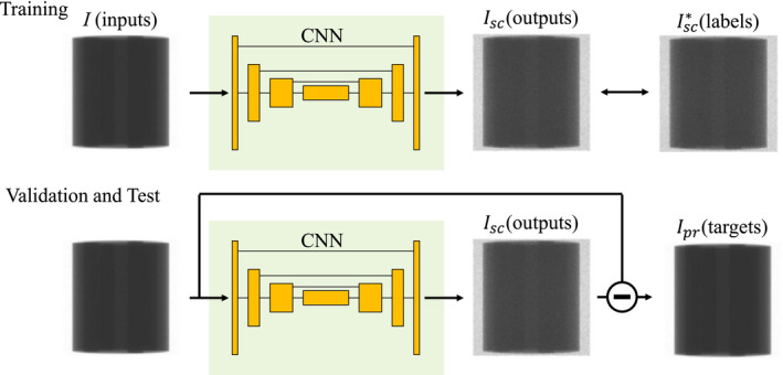
Diagram of our scatter correction workflow. Input and output were set to measured (I) and scatter‐only (Isc ) projections, respectively. illustrates label obtained using the MC simulations. During validation and test phases, subtraction of the outputs from the inputs should be scatter‐free projections Ipr. [Color figure can be viewed at wileyonlinelibrary.com]
Our CNN was trained to derive the scatter‐only projection Isc from measured projection I so that the scatter‐free (i.e., the primary) projection Ipr can be derived. Hence, we first obtain training datasets consisting of a large number of paired input and output data labeled as I and Isc , respectively, for supervised learning. Given a set of I, Isc and Ipr , we have
| (1) |
Subtraction of the output from input gives the scatter‐free projection Ipr . Although obtaining Ipr is our primary target of the task and the CNN is capable of computing them, our model was designed to output the residual scatter‐only projections Isc . This approach is generally referred to as residual learning, which performs superior to modeling the target image directly when the input and target images are close.25, 26 I is relatively closer to Ipr than Isc , and the average scatter‐to‐primary ratio over all dataset was 22.9% in this study. Therefore, the residual learning is considered to be suitable for this problem. Details of the CNN architecture are described in Section 2.C.
2.2. Monte Carlo simulation and generation of datasets
The MC simulation package GATE,27 which is wrapper codes of GEANT4,28 was used to collect projection datasets. CBCT geometry was simulated based on a CBCT machine integrated with a proton therapy system (PROBEAT‐RT, Hitachi, Japan) and listed in Table 1. The CBCT uses a flat‐panel detector (FPD) with 0.6 mm thickness of CsI crystal arrays and a 298 × 298 mm2 surface area with 372 × 372 pixels. An energy spectrum of 125 kVp CBCT x‐ray beams was calculated with a software SpekCalc.29 The focal spot size of the source was 1.2 × 1.2 mm2. Neither a bow‐tie filter nor grid was included between the source and a scanned object. Source‐to‐detector distance and source‐to‐object distance were 2178 and 1581 mm, respectively.
Table 1.
Scan geometry of simulated cone beam computed tomography (CBCT) machine
| Parameters | Values | |
|---|---|---|
| Full‐fan scans | Half‐fan scans | |
| Source‐to‐detector distance | 2178 mm | |
| Source‐to‐origin distance | 1581 mm | |
| FPD matrix | 372 × 372 | |
| FPD size | 298 × 298 mm2 | |
| Image matrix | 256 × 256 pixels × 86 slices | |
| Image size | 215 × 215 × 215 mm3 | 392 × 392 × 215 mm3 |
FPD, flat‐panel detector.
A total of 6.25 × 10⁸ photons were tracked for each projection, and the energies deposited to CsI crystal arrays and the number of scatter interaction with both the scanning object and the detector were recorded. Measured projections I were defined as accumulated energy over all detected photons, including that of the scattered photons. Scatter‐only projections Isc were calculated by summing the deposited energy from the scattered photons. Scatter‐free projections Ipr were defined as the deposited energy from the primary photons.
Five digital phantoms were constructed to generate projections for deep learning model training (Fig. 2). For each phantom, 360 projections were computed over one rotation with an interval of 1° in full‐fan scan mode. Chemical compositions of materials in the phantoms were obtained from Hudobivnik et al.30 and White et al.31 First, a cylindrical digital phantom (phantom‐1), which consists of PMMA of 18 cm in diameter and eight cylindrical inserts of air, adipose, water, breast 50/50, muscle, trabecular bone 200, bone 400, and bone 1250, was constructed. The diameter of all the inserts was 3.0 cm. The phantom‐2 was also a cylindrical PMMA phantom of the same diameter, but with five different inserts, including four bone 1250 rots, one adipose, one water, one muscle, and one breast 50/50. We note that the geometry of the phantom‐1 and phantom‐2 is the same as the CIRS phantom model 62 (CIRS, Inc., Norfolk, USA). Third, a cylindrical digital phantom (phantom‐3) of 20 cm in diameter with seven cylindrical insert rods of 2.8 cm in diameter, with the composition of muscle, adipose, water, blood, rib bone, brain, and lung tissue, respectively, was constructed. The geometry of this phantom is the same as that of the Gammex phantom (Gammex, Middleton, USA), but the material compositions are different. The length of the digital phantom‐1 to ‐3 was set to be 20 cm to accommodate the CBCT reconstruction geometry. Next, a spherical soft tissue phantom (phantom‐4) of 20 cm in diameter with eight randomly placed small spheres made of water (5.0 cm diameter), brain tissue (4.0 cm in diameter), muscle (3.0 cm), bone (3.0 cm), air (3.0 cm), lung tissue (2.0 cm), blood (2.0 cm), and adipose (1.0 cm) were constructed. The phantom‐5 was a cube phantom with the geometry of a QUASAR Penta‐Guide phantom (Modus Medical Devices Inc., London, Ontario, Canada). This phantom was made of PMMA with an inclusion of air spheres. Aliasing errors when calculating the projections from the simulations were removed by median filtering. A total of 1800 pairs of full‐fan I and Isc were generated from the five phantoms. Data augmentations were applied to the images during training, which increased training projection pairs to a total of 14 400 (see Section 2.C.).
Figure 2.
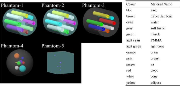
Diagrams of the phantom‐1 to ‐5 for training. Each color represents a material name listed on the right table.
For validation of the deep learning model, a digital head phantom was constructed. Two hundred projections were generated with the x‐ray source rotating from posterior to left‐anterior oblique with an interval of 1°. The phantom was generated from CT images of a head phantom (PH‐3 head phantom ACS, Kyoto Kagaku Co., Ltd., Kyoto, Japan). The CT images have a spatial resolution of 0.977 × 0.977 × 2.5 mm3/voxel, with no noticeable artifacts. After all voxel intensity outside of the phantom was set to −1000 Hounsfield Unit (HU), multilevel image thresholding was performed to categorize voxels V into air (V ≤ −400 HU), epoxy (−400 HU < V ≤ 20 HU), BRN‐SR230 (20 HU < V ≤ 130 HU), and rib bone31 (130 HU < V).
Similar to the validation datasets, two test datasets were generated (Fig. 3). First, 360 projections of an anthropomorphic digital head phantom were collected for the full‐fan test dataset. This phantom was made from a patient's treatment planning CT image dataset with all the involved structures segmented.32 The intensity outside of the body contour was assigned to be −1000 HU, and regions encompassed by the body contour were segmented into air (V ≤ −400 HU), adipose (−400 HU < V ≤ 0 HU), muscle (0 HU < V ≤ 200 HU), and rib bone (200 HU < V). Second, 360 half‐fan projections of an anthropomorphic digital lung phantom were simulated. Original CT images of a patient were selected from The Lung CT Auto‐segmentation Challenge archive33 in TCIA database.34 After removing the couch intensity manually, voxels were segmented into air (−400 HU ≤ V), adipose (−400 HU < V ≤ 0 HU), soft tissue (0 HU < V ≤ 130 HU), and rib bone (V ≤ 130 HU) except for lung. The lung volume was specifically segmented as lung tissue. Chemical compositions of each region were obtained from White et al.31
Figure 3.

Head and lung phantom diagrams. Gray‐scale images are original computed tomography image, while color images show segmented phantom image. [Color figure can be viewed at wileyonlinelibrary.com]
2.3. Network architecture and details
Figure 4 illustrates the CNN architecture used in this study. The main structure is inspired by U‐net35 that has produced remarkable results in several image regression problems.19, 36, 37 The input and output projections had the dimension of 372 × 372 × 1, and the third dimension represents channel size. Each two‐dimensional (2D) convolutional layer calculated feature map with a filter size of k and stride of 1. The padding size was set to (k−1)/2 to keep feature map dimensions unchanged. The first two 2D max pooling and the last two 2D unpooling layers had a filter size of 2 whereas others were 3. The 2D max pooling layer and the 2D unpooling layer before and after the deepest layers had a stride of 2 while others were the same as filter size. Concatenations along the channel dimension were applied between the same resolution layers to improve learning efficiency. Batch normalization38 layers were applied after each convolutional layer except for the first and the last layers. Rectified linear units (ReLU)39 layers were applied for all layers. The ReLU layer was also applied after the last convolutional layer because Isc should not have negative values. Biases in all convolutional layers followed by the batch normalizations were excluded manually because they were canceled out during normalization.
Figure 4.
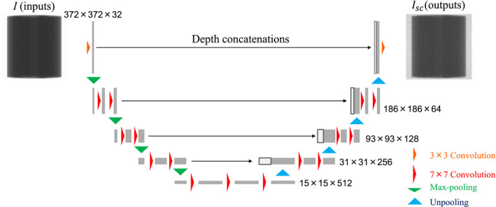
CNN architecture diagram. Yellow and red arrows represent two‐dimensional (2D) convolutional layers with filter size of 3 and 7, respectively. Green and light blue arrows indicate 2D max pooling and unpooling layers, respectively. [Color figure can be viewed at wileyonlinelibrary.com]
The CNN model was constructed using the deep neural network package Chainer40 version 4 with a GPU‐based scientific computing package CuPy.41 The CNN was trained using backpropagation with Adam optimizer42 (α = 0.001, β 1 = 0.9, β 2 = 0.999), and weight decay regularization which coefficient value was set to 10−4. Data augmentations of image 90°‐rotations and flips were randomly performed during training, which virtually increases training projection pairs to 14 400 in total.
Two different loss functions were applied for the same network structure to compare the performance of the CNN model. The mean absolute error (MAE) and mean squared error (MSE), which are commonly used as loss functions for CNN regression problems, were chosen to assess the difference from the labeled data. MAE and MSE were, respectively, computed by,
| (2) |
| (3) |
where m and n ∈ [1, mN] are mini‐batch size and pixel index, respectively. Scatter‐only intensity with * indicates the label calculated using the MC simulations. In reality, the MAE is known to find a sharper image than the MSE, whereas the MSE is robust against noise.36, 43, 44 Although some papers44, 45, 46 explored to determine the optimal loss function for a specific problem, no effective criteria have been yet proposed.
2.4. Evaluations of correction accuracy
To assess the CNN scatter correction model and effectiveness of different loss functions, Ipr of the full‐fan test dataset were compared with the actual scatter‐free projection Ipr * in four different scenarios (Table 2). The first scenario was an uncorrected case in which I was directly used. In the second scenario, Ipr calculated using an analytical scatter correction method called the fASKS‐based correction was performed (see appendix). The third scenario used Ipr obtained by the CNN trained with loss function of MSE. The fourth scenario applied Ipr with the trained CNN that has the same network architecture as that in scenario 3 but was trained with MAE. Note that all the trainings were implemented with the same initial seeds of random generators. All of the image processing and evaluations of this study were done using MATLAB version 2017b (The MathWorks Inc., Natick, MA, USA).
Table 2.
List of scenarios compared. MSE = mean squared error, MAE = mean absolute error
| Scenarios | Input projections | Loss function |
|---|---|---|
| 1 | Uncorrected | – |
| 2 | fASKS‐corrected | – |
| 3 | CNN‐corrected | MSE |
| 4 | CNN‐corrected | MAE |
| Ground truth | Scatter‐free | – |
The CNN correction model was evaluated with two different metrics. First, intensity quantification accuracy of Ipr in negative log scale was compared for the four scenarios. Because normalized negative‐logged projections are used for reconstructions, the accuracy of Ipr is much more important for reconstructed images than those in linear scale. Comparison between the scenarios 3 and 4 shows which loss function is sensitive to the difference in negative log scale. Both MAE and MSE consider the difference between the output and the label in linear scale [Fig. 5(a)]. When they are regarded with respect to the differences in negative‐logged scatter‐free projections Δnlog, Eqs. (2) and (3) are rewritten by,
| (4) |
| (5) |
Figure 5.
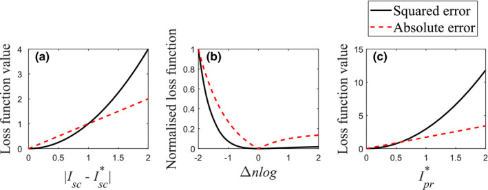
Comparisons of absolute and squared errors. Figure (a) shows the loss functions with function of linear difference. Figure (b) compares normalized loss functions with function of negative‐logged difference. Figure (c) illustrates the loss functions with function of the real scatter‐free projection at Δnlog = −1. [Color figure can be viewed at wileyonlinelibrary.com]
| (6) |
These equations suggest that the absolute and squared errors are functions of linear and squared , respectively [Figs. 5(b) and 5(c)]. The second metric was the comparison between reconstructed images from Ipr and . Median filtering with a filter size of 5 × 5 was applied for all projections before image reconstruction to reduce noise. The Feldkamp–Davis–Kress reconstruction method with the Hanning filter was applied for all scenarios using a GPU‐based CBCT reconstruction toolbox TIGRE.47 These images were then converted to HU by,
| (7) |
where μ denotes the reconstructed linear attenuation coefficient images. μw indicates the reference water intensity and calculated by the scatter‐free reconstructed images of the phantom‐1. The CNN‐corrected reconstructed images were further evaluated by comparing with the fASKS‐corrected images using four different quality measures; MAE, MSE, peak signal‐to‐noise ratio (PSNR) and structural similarity (SSIM).48 The PSNR and SSIM are calculated by,
| (8) |
| (9) |
| (10) |
where μX and denote the mean and variance of X, respectively. σXY is the covariance of X and Y. max() returns the maximum pixel value of . l is a dynamic range of projection images and was set to (216−1) in this study. These measures were calculated over all slices, and paired t‐test was performed for each measure to assess statistical significance between CNN‐corrected and fASKS‐corrected images. A value of P < 5% was considered to be statistically significant in this study.
2.5. Transfer learning of trained CNN model with half‐fan projections
To demonstrate the capability of the CNN model for different scan conditions, the CNN model trained with the full‐fan projection pairs was fine‐tuned with a small amount of half‐fan projections for scatter correction of large‐sized patients. To generate additional training datasets for half‐fan scans, four new phantoms were constructed by making two different modifications to the phantom‐1 to ‐3. The diameter of these phantoms was extended to 35.0 × 30.0 cm2, and the diameter of the phantom‐3 was extended to 25.0 × 20.0 cm2. 60 half‐fan projections of the modified phantoms, phantom‐4 and phantom‐5, were collected over one rotation with an interval of 6°, providing 360 projection pairs in total. Assuming that the CNN model trained for full‐fan projections is capable of extracting enough features to reconstruct half‐fan Isc , the parameters of last two convolutional layers and the last batch normalization layer were tuned, while other parameters were kept unchanged during training. To moderate learning rate, the α value in the Adam optimizer was changed to 10−5. Data augmentation of image flips perpendicular to the rotation axis was randomly performed. Other training strategies for the transfer learning are the same as those in the Section 2.C. To evaluate the impact of the transfer learning, the accuracy of the test lung phantom images corrected using the CNN models with and without the transfer learning were compared.
3. Results
3.1. Comparisons of scatter‐corrected projections in negative‐logged scale
Figure 6 shows training curves of the scenarios 3 and 4 with MAE values of the full‐fan validation dataset. The training loss values of both scenarios converge well, despite of the fluctuating behavior during training. The CNN was trained for 100 epochs with a mini‐batch size of 10 for both scenarios. Computation time for the training was about 10 h with a PC installing single NVIDIA GTX 1070 GPU and 4.20 GHz Intel Core‐i7 CPU. Computation time required to correct 360 projections is approximately 4.8 s with the same PC.
Figure 6.
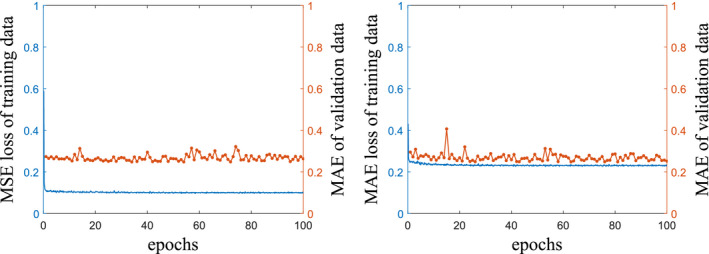
Training curves of the scenarios 3 (left) and 4 (right). Solid blue lines are loss function values of training data, and dotted orange lines illustrate MAE values of the validation data during training. [Color figure can be viewed at wileyonlinelibrary.com]
Figure 7 compares the model calculation with the ground truth in negative log scale for different scenarios. The difference maps between the two are also displayed for two projection angles. Because of scatter contamination, the scenario 1 has negative errors, especially in high intensity regions. In the scenario 2, the accuracy of projection intensity in the soft tissue regions is improved. However, as can be seen from the second angle in Fig. 7, accurate prediction of scatter contributions in the bony regions remains challenging because the fASKS method assumes that all of the scanned materials are made of water or water‐equivalent materials. In the scenario 3, the image is less noisy, but the accuracy in the bony regions is worse than that of the scenario 2. The CNN model in the scenario 4 leads to markedly improvement in quantification accuracy. Almost all of the negative errors disappear. Root mean squared errors of 360 projection intensities against the ground truth in negative log scale were 0.278, 0.117, 0.100, and 0.0862 for the scenarios 1–4, respectively.
Figure 7.
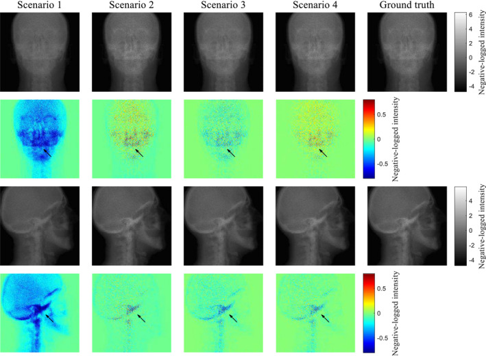
Comparison of the scatter‐corrected projections with the ground truths in negative log scale for two projection angles. Color maps on the bottom row represent difference maps against the ground truths. [Color figure can be viewed at wileyonlinelibrary.com]
To further evaluate the influence of loss function on the performance of CNN‐based scatter correction, all projection pixels were categorized into five groups according to intensity [Fig. 8(a)]. For each group, mean squared errors of Ipr with respect to in scenarios 3 and 4 were compared. In both scenarios, the mean squared errors at low intensity groups are relatively large due to the existence of large photon noise [Fig. 8(b)]. However, smaller errors were observed at low groups in scenario 4 than scenario 3. In general, it seems that the MAE is more sensitive loss function to errors at low as compared to the MSE.
Figure 8.
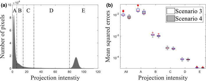
(a) Histogram of pixel intensity. Dotted lines illustrate thresholds of different groups for (b). Figure (b) shows box plots of mean squared errors over projection. Each category along the x‐axis indicates group whereas “All” covers all projection pixels. Central red lines indicate medians, and box edges are 25%/75% percentiles. Outliers were marked as red crosses independently. [Color figure can be viewed at wileyonlinelibrary.com]
3.2. Scatter‐corrected reconstruction
Figure 9 shows the scatter‐corrected reconstructed images together with the ground truth images in two different slices. The HU value around the image center is lower in scenario 1 than that in the ground truth, which is often called cupping artifact caused by the scatter. Furthermore, the scenario 1 has noticeable errors in low or high intensity areas such as the nasal cavity and bone. In contrast, the HU value accuracy is visually improved in the scenario 2, but it contains a negative error as well as streaking artifacts at bony structure. Similarly, the scenario 3 has no cupping artifacts, but is contaminated by localized errors in air cavities and bony structures. A uniform negative error inside of the phantom is observed. In scenario 4, almost all of the artifacts and regional errors are not observed. HU value difference is close to zero among all pixels. These results demonstrate that the CNN model can correct for scatter with high accuracy and provides images that are visually comparable to the scatter‐free images.
Figure 9.
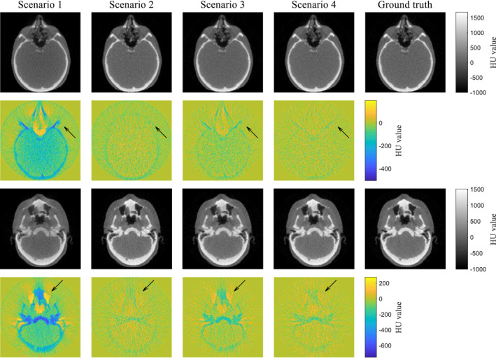
Comparison of the scatter‐corrected reconstructed images with the ground truths in two different slices. Color maps illustrate difference maps against the ground truths. [Color figure can be viewed at wileyonlinelibrary.com]
The scatter‐corrected images shown in the first slice in Fig. 9 were further compared quantitatively. The histogram of HU difference (Fig. 10) indicates that the median values are −54.7, −13.1, −8.38, and −1.60 HU, respectively, for the scenarios 1–4. A long, negative tail observed in the histogram of scenario 1 is a reflection of the cupping artifact. The histogram of scenario 2 has a narrower width, but its center is shifted to negative, indicating that the fASKS correction improves HU value precision but not the accuracy of HU value. The negative tail of scenario 3 indicates that the HU value inside of the phantom or in the bony structures is lower than that of the ground truth. The scenario 4 has a narrow width and a median value close to 0. The scatter‐corrected images at other slices show similar results as Fig. 10. Since the scenario 4 provides the best accuracy, we will focus on the CNN model with the MAE loss function in the following.
Figure 10.
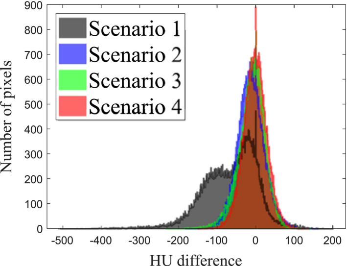
Histograms of the Hounsfield Unit intensity difference for different study scenarios illustrated at the second row of Fig. 9. Pixels outside of field‐of‐view were excluded.
The image quality of the CNN‐based reconstruction (scenario 4) is further compared with the fASKS calculation (scenario 2) using four image quality measures (Table 3). All of the measures show that the CNN‐corrected images lead to better image quality. These results indicate that the CNN‐based reconstruction can accurately represent the scatter‐free reconstructed images.
Table 3.
Comparison of image quality of the head phantom images between the fast adaptive scatter kernel superposition (fASKS) and convolutional neural network (CNN) corrections (mean + SD). Mean absolute error (MAE), mean squared error (MSE), peak signal‐to‐noise ratio (PSNR) and structural similarity (SSIM) were used
| MAE (HU) | MSE (HU2) | PSNR (dB) | SSIM | |
|---|---|---|---|---|
| fASKS | 21.8 ± 5.9 | 1069 ± 613 | 35.6 ± 2.3 | 0.9995 ± 0.0003 |
| CNN | 17.9 ± 5.7 | 779 ± 511 | 37.2 ± 2.6 | 0.9997 ± 0.0003 |
| P‐value | 1.38 × 10⁻⁵ | 9.13 × 10⁻⁴ | 6.27 × 10⁻⁵ | 9.48 × 10⁻⁷ |
3.3. Transfer learning and its impact on correction accuracy
The transfer learning was applied to the trained CNN model of scenario 4. The CNN was trained for 15 epochs with loss function of MAE using the half‐fan training dataset. The CNN‐corrected images with and without the transfer learning are shown in Fig. 11. The CNN model without tuning provides more accurate images than the uncorrected images although it was trained only with the half‐fan projection pairs. The tuned‐CNN‐corrected images have better HU value accuracy and less artifacts than the non‐tuned‐CNN or the fASKS‐corrected images. Comparison of the four image quality metrics further indicates that the tuned CNN model outperforms both fASKS and non‐tuned CNN models with high statistical significance (Table 4). These results show that the trained CNN model is expandable for other scan conditions with transfer learning.
Figure 11.
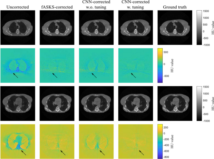
Comparison of the scatter‐corrected lung phantom images with the ground truths for two different slices. Two different convolutional neural network (CNN)‐corrected images, obtained using the scenario 4 CNN model with and without the transfer learning, are shown. Color maps illustrate difference maps against the ground truths. [Color figure can be viewed at wileyonlinelibrary.com]
Table 4.
Comparison of image quality of the lung phantom images between the tuned‐convolutional neural network (CNN) correction and the fast adaptive scatter kernel superposition (fASKS) and non‐tuned‐CNN corrections (mean + SD). Mean absolute error (MAE), mean squared error (MSE), peak signal‐to‐noise ratio (PSNR) and structural similarity (SSIM) over central 70 slices were used
| MAE (HU) | MSE (HU2) | PSNR (dB) | SSIM | |
|---|---|---|---|---|
| fASKS | 32.5 ± 3.2 | 2423 ± 559 | 30.6 ± 0.9 | 0.9990 ± 0.0003 |
| CNN w.o. tuning | 31.8 ± 3.8 | 2699 ± 974 | 30.2 ± 1.2 | 0.9984 ± 0.0005 |
| CNN w. tuning | 29.0 ± 2.5 | 1882 ± 376 | 31.7 ± 0.8 | 0.9993 ± 0.0002 |
| P‐value (vs fASKS) | 2.41 × 10⁻¹¹ | 4.72 × 10⁻¹⁰ | 1.71 × 10⁻¹² | 6.98 × 10⁻¹⁷ |
| P‐value (vs CNN w.o. tuning) | 5.91 × 10⁻⁷ | 1.11 × 10⁻⁹ | 7.36 × 10⁻¹⁵ | 2.80 × 10⁻³² |
4. Discussion
This study establishes a projection‐domain scatter correction technique for CBCT using a residual CNN. The CNN‐corrected projection offers more accurate intensity quantification and better image quality than the conventional fASKS approach. The deep learning‐based approach is able to take prior knowledge into account efficiently and correct for scatter contamination in the projections of the various imaged subject. By avoiding using any handcrafted features, CNN is able to learn and provide a sophisticated scatter correction model without any assumptions. Once trained, the method is computationally efficient, taking around 13 ms per projection on a desktop computer with a single GPU.
We compared the performance of CNN model with two major loss functions and found that MAE outperforms MSE in recognizing negative‐logged intensity difference Δnlog from the label. Although the loss functions of the negative‐logged output from the negative‐logged label can penalize Δnlog, they were not successful in our experiments because logarithm computation amplifies photon noise in the label and it degrades the training efficiency. Label noise should be taken into consideration for determining appropriate loss functions.49 Though the final results are dependent on various other factors such as quality of dataset, optimizer, or training strategy, one possible reason responsible for the performance variations is that MAE and MSE are differently weighted by in negative log scale [Eqs. (4) and (5)]. As illustrated in Fig. 5, the squared error is prominent at high , which occurs mainly at pixels less attenuating, whereas the same Δnlog at pixels with low is not penalized well. In contrast, the absolute error is less dependent on than the squared error and can better penalize Δnlog at low . This explains why the scenario 3 has both larger error at pixels with lower than scenario 4 [Fig. 8(b)] and the negative error inside of the phantom in the reconstructed images (Fig. 9). To assess the impact of Ipr * in the loss functions to the residual errors, we introduce a loss function L,
| (11) |
where λ is a parameter to control the weight of . The same CNN trainings were performed with a few different values of λ, ranging from 0, which is the original MSE, to 5, with an interval of 1, and the calculated Ipr were compared with . As illustrated in Fig. 12, the projection is degraded especially at high with increasing λ. Projections at other gantry angles behave similarly. The selection of loss functions is generally a challenging46, 49, 50 task, and needs to be refined in the future.
Figure 12.
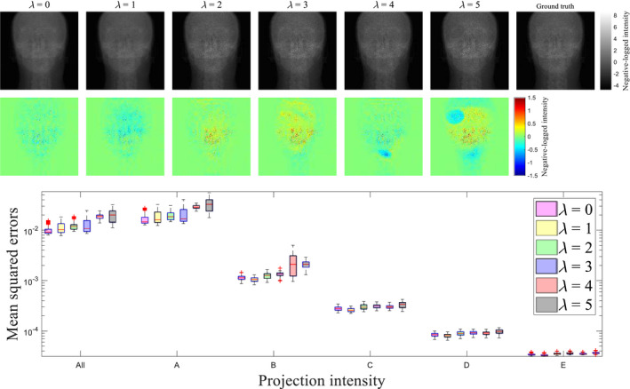
(top) Projection images obtained using with different λ's. Color maps illustrate difference of the projection against the ground truth. (bottom) Comparison of mean squared errors over all test data with different λ's. Category along the x‐axis indicates the same groups as that in Fig. 8. Central red lines indicate medians, and box edges are 25%/75% percentiles. Outliers were marked as red crosses independently.
The novelty of this study is reflected in four aspects. First, our CNN model corrects both scatter and glare, while other studies correct only scatter. Since the glared intensity can be removed only using software‐based scatter estimation techniques,1, 8 our CNN model is unique in this aspect. Second, this study indicates that the features characterizing scatter distributions in anthropomorphic phantoms can be learned from nonanthropomorphic digital phantom projections. Some previous studies19, 24 investigated using image pairs of patients for CNN‐based image synthesis or restoration. It was noted that a difficulty in using the patient dataset is that the paired images are not always matched because of body movement or time lag between images. Although the problem can, in principle, be solved by applying image registration, it is difficult to guarantee that all image pairs are perfectly matched.19 Moreover, the MC simulations of patient images require rough approximations of body density and chemical compositions, which may cause uncertainty in labeling the scatter‐only projections.51 These mismatched pairs adversely influence the accuracy of learning and inference. Nonanthropomorphic phantoms are, on the other hand, static and made of known materials, and it is not necessary to prealign the image pairs. Scanning of the phantom with various scanning conditions is fairly straightforward and expand the distribution of training dataset. Learning by using nonanthropomorphic phantom data thus improves the quality of training dataset. Third, our study provides an effective criterion for selecting appropriate loss functions for deep learning‐based corrections in projection domain. Although this study only focuses on the CBCT‐based scatter correction, the criterion can be applied to other projection‐domain corrections and other imaging modalities such as SPECT or PET. Finally, we evaluated the feasibility of transfer learning for large field‐of‐view (FOV) scans by fine‐tuning a CNN model obtained using smaller phantoms.
This study applied scatter correction in the projection domain. Scatter correction in the image domain can also be accomplished.16, 17, 37 In general, projection‐domain scatter correction is advantageous for three reasons. First, the thickness of the attenuation object is important for scatter estimation as the scatter‐to‐primary ratio increases with the thickness. The reconstructed image does not provide the thickness for photons passing through multiple slices. Projection domain calculation takes the volumetric contributions of scatter photons more accurately. Second, the projection‐domain correction is well‐adjusted to the network structure of CNN. CNN is designed to connect only center and surrounding neurons to enhance feature localizations and learning efficiency.52, 53 It hence provides superior results for problems in which information required for inference is localized like image deblurring,54 super‐resolution,14, 15 and denoising.16, 17 Scatter effects generally appear in a wide area of images and are difficult to be inferred using a small area in image domain. In contrast, scatter in a projection is well localized, and input pixel values have a much larger influence on the inference of the output pixel values at the same position. Finally, the number of projections is generally larger than reconstructed images for one scan. The number of reconstructed images is limited by FOV, and thin slice thickness increases the image number but leads to image noise. The projection number is easily increased with a smaller rotation interval, and projection quality is independent of the number of projection. This advantage also holds for other CBCT problems including beam hardening, metal artifacts and CBCT‐FBCT image synthesis.
We have only used MC simulations instead of real experimental data for evaluation. The scatter‐only or scatter‐free projections are not attainable in CBCT experiments. Available solutions are to use projections calculated by pre‐evaluated MC simulations,23 to use higher quality images like fan‐beam CT images24 or to apply image‐to‐image translation networks with unsupervised learning.18, 55, 56 Our MC simulation setups were referenced from specifications of a real CBCT machine, but the FPD grid was not considered because the data were not available. The best solution should use projections considering all the geometrical parameters of the imaging system during the training of CNN model. When the grid information are available, the grid effect on the input projections can be removed using theoretical models10, 57 before applying the CNN correction. When the grid is completely unknown as in this study, the trained CNN model needs to be fine‐tuned to adjust for actual scans. Interpretations of all hyperparameters in the CNN is very difficult because, unlike other machine learning algorithms, each hyperparameter do not have effective correspondence (or meanings) to the final results. Thus, their transparency is not easily available. Interpretability of the deep learning techniques is still a challenge and there are progressive efforts in mitigating the “black box” nature of neural network.58, 59
5. Conclusion
We developed an effective CBCT scatter correction method using residual CNN. We demonstrated that the CNN‐corrected reconstruction outperforms the conventional fASKS‐based method. Computation of the model is fast and suitable for real‐time clinical use. This technique promises to provide scatter‐free CBCT images for IGRT and adaptive radiation therapy.
Conflict of interest
The authors have no relevant conflict of interest to disclose.
Acknowledgments
This work was partially supported by NIH (1R01 CA227713 and 1R01 CA223667).
Appendix A1.
FAST adaptive scatter kernel superposition model
The fASKS correction10 is one of the conventional projection‐domain scatter estimation methods. It has a model in which scatter intensity Isc of each projection is convolutional intensity of primary intensity Ipr with an adaptive scatter kernel hs .
| (A1) |
| (A2) |
where Φ denotes the sensitive detector area. Symmetric scatter kernel adapts to various thickness of a scanned object and varies according to water‐equivalent thickness (WET) τ of photon beams. i represents the number of symmetric scatter kernels and R is a weighting function switching the symmetric scatter kernels. Each symmetric kernel is composed of an amplitude factor c and a form‐function g. A parameter γ is an adaptive factor of symmetric scatter kernels. This model also considered glare, and its effect is also represented using a filter called glare kernel. Final measured intensity I is, therefore, modeled as,
| (A3) |
where hg is a glare kernel. The scatter and glare kernels should be obtained before taking scans and are mainly obtained by either MC simulations or experiments.60 The fASKS model assumes that all of the scanned materials are made of water or water‐equivalent materials. In this study, in‐house fASKS correction61 with scatter and glare kernels acquired using edge‐spread function measurements were performed. γ was set to 0.02 that was the optimal value for intensity uniformity in reconstructed images of water cylinder phantoms. Computation time of the fASKS method required to correct 360 projections is around 5.5 min with our equipment.
Nomura Y, Xu Q, Shirato H, Shimizu S, Xing L. Projection‐domain scatter correction for cone beam computed tomography using a residual convolutional neural network. Med. Phys.. 2019;46:3142–3155. 10.1002/mp.13583
Contributor Information
Yusuke Nomura, Email: yusuke_n-medphyz15@eis.hokudai.ac.jp.
Lei Xing, Email: lei@stanford.edu.
References
- 1. Poludniowski G, Evans PM, Kavanagh A, Webb S. Removal and effects of scatter‐glare in cone‐beam CT with an amorphous‐silicon flat‐panel detector. Phys Med Biol. 2011;56:1837–1851. [DOI] [PubMed] [Google Scholar]
- 2. Poludniowski G, Evans PM, Hansen VN, Webb S. An efficient Monte Carlo‐based algorithm for scatter correction in keV cone‐beam CT. Phys Med Biol. 2009;54:3847–3864. [DOI] [PubMed] [Google Scholar]
- 3. Lazos D, Williamson JF. Monte Carlo evaluation of scatter mitigation strategies in cone‐beam CT. Med Phys. 2010;37:5456–5470. [DOI] [PMC free article] [PubMed] [Google Scholar]
- 4. Sisniega A, Zbijewski W, Badal A, et al. Monte Carlo study of the effects of system geometry and antiscatter grids on cone‐beam CT scatter distributions. Med Phys. 2013;40:051915. [DOI] [PMC free article] [PubMed] [Google Scholar]
- 5. Rührnschopf and E‐P, Klingenbeck K. A general framework and review of scatter correction methods in cone beam CT. Part 2: Scatter estimation approaches. Med Phys. 2011;38:5186–5199. [DOI] [PubMed] [Google Scholar]
- 6. Ning R, Tang X, Conover D. X‐ray scatter correction algorithm for cone beam CT imaging. Med Phys. 2004;31:1195–1202. [DOI] [PubMed] [Google Scholar]
- 7. Zhu L, Xie Y, Wang J, Xing L. Scatter correction for cone‐beam CT in radiation therapy. Med Phys. 2009;36:2258–2268. [DOI] [PMC free article] [PubMed] [Google Scholar]
- 8. Lazos D, Williamson JF. Impact of flat panel‐imager veiling glare on scatter‐estimation accuracy and image quality of a commercial on‐board cone‐beam CT imaging system. Med Phys. 2012;39:5639–5651. [DOI] [PMC free article] [PubMed] [Google Scholar]
- 9. Ohnesorge B, Flohr T, Klingenbeck‐Regn K. Efficient object scatter correction algorithm for third and fourth generation CT scanners. Eur Radiol. 1999;9:563–569. [DOI] [PubMed] [Google Scholar]
- 10. Sun M, Star‐Lack JM. Improved scatter correction using adaptive scatter kernel superposition. Phys Med Biol. 2010;55:6695–6720. [DOI] [PubMed] [Google Scholar]
- 11. Simonyan K, Zisserman A. Very Deep Convolutional Networks for Large‐Scale Image Recognition. arXiv. September 2014:1–14. http://arxiv.org/abs/1409.1556
- 12. Dou Q, Yu L, Chen H, et al. 3D deeply supervised network for automated segmentation of volumetric medical images. Med Image Anal. 2017;41:40–54. [DOI] [PubMed] [Google Scholar]
- 13. Ibragimov B, Xing L. Segmentation of organs‐at‐risks in head and neck CT images using convolutional neural networks. Med Phys. 2017;44:547–557. [DOI] [PMC free article] [PubMed] [Google Scholar]
- 14. Dong C, Loy CC, He K, Tang X. Image super‐resolution using deep convolutional networks. IEEE Trans Pattern Anal Mach Intell. 2016;38:295–307. [DOI] [PubMed] [Google Scholar]
- 15. Liu H, Xu J, Wu Y, Guo Q, Ibragimov B, Xing L. Learning deconvolutional deep neural network for high resolution medical image reconstruction. Inf Sci (NY). 2018;468:142–154. [Google Scholar]
- 16. Chen H, Zhang Y, Kalra MK, et al. Low‐dose CT With a Residual Encoder‐Decoder Convolutional Neural network. IEEE Trans Med Imaging. 2017;36:2524–2535. [DOI] [PMC free article] [PubMed] [Google Scholar]
- 17. Wolterink JM, Leiner T, Viergever MA, Isgum I. Generative adversarial networks for noise reduction in low‐dose CT. IEEE Trans Med Imaging. 2017;36:2536–2545. [DOI] [PubMed] [Google Scholar]
- 18. Wolterink JM, Dinkla AM, Savenije MHF, Seevinck PR, van den Berg CAT, Išgum I. Deep MR to CT Synthesis Using Unpaired Data. In: Lecture Notes in Computer Science (Including Subseries Lecture Notes in Artificial Intelligence and Lecture Notes in Bioinformatics). Vol 10557 LNCS; 2017:14–23. 10.1007/978-3-319-68127-6_2 [DOI]
- 19. Han X. MR‐based synthetic CT generation using a deep convolutional neural network method. Med Phys. 2017;44:1408–1419. [DOI] [PubMed] [Google Scholar]
- 20. Leung K, Marashdeh W, Wray R, et al. A deep‐learning‐based fully automated segmentation approach to delineate tumors in FDG‐PET images of patients with lung cancer. J Nucl Med. 2018;59:323. [Google Scholar]
- 21. Henry T, Chevance V, Roblot V, et al. Automated PET segmentation for lung tumors: can deep learning reach optimized expert‐based performance? J Nucl Med. 2018;59:322. [Google Scholar]
- 22. Xing L, Krupinski EA, Cai J. Artificial intelligence will soon change the landscape of medical physics research and practice. Med Phys. 2018;45:1791–1793. [DOI] [PMC free article] [PubMed] [Google Scholar]
- 23. Maier J, Sawall S, Knaup M, Kachelrieß M. Deep scatter estimation (DSE): accurate real‐time scatter estimation for x‐ray CT using a deep convolutional neural network. J Nondestruct Eval. 2018;37:57. [Google Scholar]
- 24. Hansen DC, Landry G, Kamp F, et al. ScatterNet: aA convolutional neural network for cone‐beam CT intensity correction. Med Phys. 2018;45:4916–4926. [DOI] [PubMed] [Google Scholar]
- 25. He K, Zhang X, Ren S, Sun J. Deep residual learning for image recognition. In: Proceedings of the IEEE Conference on Computer Vision and Pattern Recognition; 2016:770–778.
- 26. Zhang K, Zuo W, Chen Y, Meng D, Zhang L. Beyond a Gaussian denoiser: residual learning of deep CNN for image denoising. IEEE Trans Image Process. 2017;26:3142–3155. [DOI] [PubMed] [Google Scholar]
- 27. Jan S, Benoit D, Becheva E, et al. GATE V6: a major enhancement of the GATE simulation platform enabling modelling of CT and radiotherapy. Phys Med Biol. 2011;56:881–901. [DOI] [PubMed] [Google Scholar]
- 28. Allison J, Amako K, Apostolakis J, et al. Recent developments in Geant 4. Nucl Instrum Methods Phys Res Sect A Accel Spectrom Detect Assoc Equip. 2016;835:186–225. [Google Scholar]
- 29. Poludniowski G, Landry G, DeBlois F, Evans PM, Verhaegen F. SpekCalc: a program to calculate photon spectra from tungsten anode x‐ray tubes. Phys Med Biol. 2009;54:N433–N438. [DOI] [PubMed] [Google Scholar]
- 30. Hudobivnik N, Schwarz F, Johnson T, et al. Comparison of proton therapy treatment planning for head tumors with a pencil beam algorithm on dual and single energy CT images. Med Phys. 2016;43:495–504. [DOI] [PubMed] [Google Scholar]
- 31. White DR, Woodard HQ, Hammond SM. Average soft‐tissue and bone models for use in radiation dosimetry. Br J Radiol. 1987;60:907–913. [DOI] [PubMed] [Google Scholar]
- 32. Craft D, Bangert M, Long T, Papp D, Unkelbach J. Shared data for intensity modulated radiation therapy (IMRT) optimization research: the CORT dataset. Gigascience. 2014;3:37. [DOI] [PMC free article] [PubMed] [Google Scholar]
- 33. Yang J, Veeraraghavan H, Armato SG, et al. Autosegmentation for thoracic radiation treatment planning: a grand challenge at AAPM 2017. Med Phys. 2018;45:4568–4581. [DOI] [PMC free article] [PubMed] [Google Scholar]
- 34. Clark K, Vendt B, Smith K, et al. The cancer imaging archive (TCIA): maintaining and operating a public information repository. J Digit Imaging. 2013;26:1045–1057. [DOI] [PMC free article] [PubMed] [Google Scholar]
- 35. Ronneberger O, Fischer P, Brox T. U‐Net: convolutional networks for biomedical image segmentation. In: Navab N, Hornegger J, Wells WM, Frangi AF, eds. Medical Image Computing and Computer‐Assisted Intervention – MICCAI 2015. Cham: Springer International Publishing; 2015:234–241. [Google Scholar]
- 36. Isola P, Zhu J‐Y, Zhou T, Efros AA. Image‐to‐Image Translation with Conditional Adversarial Networks. arXiv. November 2016. http://arxiv.org/abs/1611.07004
- 37. Jin KH, McCann MT, Froustey E, Unser M. Deep convolutional neural network for inverse problems in imaging. IEEE Trans Image Process. 2017;26:4509–4522. [DOI] [PubMed] [Google Scholar]
- 38. Ioffe S, Batch Szegedy C. Normalization: Accelerating Deep Network Training by Reducing Internal Covariate Shift. arXiv. February 2015. http://arxiv.org/abs/1502.03167
- 39. Nair V, Hinton GE. Rectified linear units improve restricted Boltzmann machines. Proc 27th Int Conf. Mach Learn; 2010:807–814.
- 40. Tokui S, Oono K, Hido S, Clayton J. Chainer: a next‐generation open source framework for deep learning. In: Proceedings of Workshop on Machine Learning Systems (LearningSys) in the Twenty‐Ninth Annual Conference on Neural Information Processing Systems (NIPS). Vol 5; 2015:1–6.
- 41. Okuta R, Unno Y, Nishino D, Hido S, Loomis C CuPy: NumPy‐Compatible Library for NVIDIA GPU Calculations. In: Proceedings of Workshop on Machine Learning Systems (LearningSys) in The Thirty‐First Annual Conference on Neural Information Processing Systems (NIPS); 2017.
- 42. Kingma DP, Ba J.Adam: A Method for Stochastic Optimization. arXiv. 2014;33:2698–2704.
- 43. Ledig C, Theis L, Huszar F, et al. Single Image Super‐Resolution Using a Generative Adversarial Network. 2017 IEEE Conference on Computer Vision and Pattern Recognition (CVPR). IEEE. 2017;105–114. [Google Scholar]
- 44. Zhao H, Gallo O, Frosio I, Kautz J. Loss functions for image restoration with neural networks. IEEE Trans Comput Imaging. 2017;3:47–57. [Google Scholar]
- 45. Lorbert A, Ben‐Zvi N, Ciptadi A, Oks E, Tyagi A. Toward better reconstruction of style images with GANs. KDDW ML meets Fash; 2017.
- 46. Barron JTA. General and Adaptive Robust Loss Function. arXiv; 2017:1(5). http://arxiv.org/abs/1701.03077
- 47. Biguri A, Dosanjh M, Hancock S, Soleimani M. TIGRE: a MATLAB‐GPU toolbox for CBCT image reconstruction. Biomed Phys Eng Express. 2016;2:055010. [Google Scholar]
- 48. Wang Z, Bovik AC, Sheikh HR. Image quality assessment: from error measurement to structural similarity. IEEE Trans Image Process. 2004;13:600–612. [DOI] [PubMed] [Google Scholar]
- 49. Barbu A, Lu L, Roth H, Seff A, Summers RM. An analysis of robust cost functions for CNN in computer‐aided diagnosis. Comput Methods Biomech Biomed Eng Imaging Vis. 2018;6:253–258. [Google Scholar]
- 50. Janocha K, Czarnecki WM On Loss Functions for Deep Neural Networks in Classification. arXiv. February 2017. http://arxiv.org/abs/1702.05659
- 51. Verhaegen F, Devic S. Sensitivity study for CT image use in Monte Carlo treatment planning. Phys Med Biol. 2005;50:937–946. [DOI] [PubMed] [Google Scholar]
- 52. Bach S, Binder A, Montavon G, et al. Pixel‐wise explanations for non‐linear classifier decisions by layer‐wise relevance propagation. PLoS ONE. 2015;10:e0130140. [DOI] [PMC free article] [PubMed] [Google Scholar]
- 53. Luo W, Li Y, Urtasun R, Zemel R. Understanding the Effective Receptive Field in Deep Convolutional Neural Networks. In: Lee DD, Sugiyama M, Luxburg UV, Guyon I, Garnett R, eds. Advances in Neural Information Processing Systems 29. Red Hook, NY: Curran Associates Inc; 2016:4898–4906. http://papers.nips.cc/paper/6203-understanding-the-effective-receptive-field-in-deep-convolutional-neural-networks.pdf [Google Scholar]
- 54. Xu L, Ren JSJ, Liu C, Jia J. Deep Convolutional Neural Network for Image Deconvolution. In: Ghahramani Z, Welling M, Cortes C, Lawrence ND, Weinberger KQ, eds. Advances in Neural Information Processing Systems 27. Red Hook, NY: Curran Associates Inc; 2014:1790–1798. [Google Scholar]
- 55. Zhu J‐Y, Park T, Isola P, Efros AA. Unpaired Image‐to‐Image Translation using Cycle‐Consistent Adversarial Networks. Comput Vis (ICCV), 2017 IEEE Int Conf; 2017:2223–2232.
- 56. Yi Z, Zhang H, Tan P, Gong M. DualGAN: Unsupervised Dual Learning for Image‐to‐Image Translation. In: 2017 IEEE International Conference on Computer Vision (ICCV). Vol 2017‐Octob. IEEE; 2017:2868–2876.
- 57. Day GJ, Dance DR. X‐ray transmission formula for antiscatter grids. Phys Med Biol. 1983;28:1429–1433. [DOI] [PubMed] [Google Scholar]
- 58. Ancona M, Ceolini E, Öztireli C, Gross M. Towards better understanding of gradient‐based attribution methods for deep neural networks; 2017;3142–16.
- 59. Samek W, Binder A, Montavon G, Lapuschkin S, Muller K‐R. Evaluating the visualization of what a deep neural network has learned. IEEE Trans Neural Networks Learn Syst. 2017;28:2660–2673. [DOI] [PubMed] [Google Scholar]
- 60. Li H, Mohan R, Zhu XR. Scatter kernel estimation with an edge‐spread function method for cone‐beam computed tomography imaging. Phys Med Biol. 2008;53:6729–6748. [DOI] [PubMed] [Google Scholar]
- 61. Nomura Y, Xu Q, Peng H, Shirato H, Shimizu S, Xing L. Evaluation of Scatter Correction with Modified Scatter Kernel Model for CBCT‐based Radiotherapy: MO‐L‐GEPD‐J (a)‐05. Med Phys. 2017;44:3051. [Google Scholar]


